Abstract
Air-sea fluxes have rarely or never been estimated from in situ observations in many parts of the global oceans, especially in the Arctic, despite their critical roles in weather and climate. In consequence, their reproductions by numerical models have seldomly been validated against observations. In this study, observations from Saildrone Explorer uncrewed surface vehicles are used to validate surface sensible and latent heat fluxes from GFS deterministic forecasts and GEFS ensemble forecasts in the Arctic during May – October 2019. The most striking result from this study is the low biases in sea surface temperature (SST) in the initial conditions of both the deterministic and ensemble forecasts. Excessively cold predictions of SST lead to reversed signs in air-sea differences in temperature and humidity in comparison to the observations. Consequently, surface sensible and latent heat fluxes in the forecast can be negative (from air into the water), while observed fluxes are positive. The larger SST biases at the initial time og the GEFS ensemble forecasts is the main reason for their underperformance in comparison to the GFS deterministic forecasts. The results clearly demonstrate the vital step of improving forecasts in the Arctic is to prepare for accurate initial conditions of SST.
1 Introduction
The Arctic is warming at a rate approximately four times faster than the global average, a phenomenon known as Arctic amplification, driving significant changes within the Arctic environment and throughout the world (Rantanen et al., 2022). Sensible and latent heat fluxes at the air-sea interface are critical components of energy balance in the Arctic. The temperature-driven (sensible) and phase change-driven (latent) exchanges of heat between the ocean and atmosphere affect sea ice melt and ocean temperatures, consequently influencing broader climate patterns (Overland et al., 2011; Walsh, 2014; Kug et al., 2015; Yamanouchi and Takata, 2020). Exchanges of energy at the air-sea interface are determined by the contrasts between ocean and air temperatures and by surface wind speeds, both generating turbulence. As sea ice declines, the total area of ocean surface exposed to and interacting with the atmosphere increases. This alters the exchange of heat and water vapor at the air-sea interface, and increases the ocean absorption of shortwave radiation and release of longwave radiation (Serreze et al., 2009; Dai, 2021). The release of heat from the ocean after sea ice retreat is the primary driver of surface air warming in the Arctic (Dai and Jenkins, 2023). Atmospheric warming then delays ice formation in the cold season in a positive feedback loop referred to as ice-albedo feedback (Dai and Jenkins, 2023), increasing year-round open ocean area at which these fluxes occur.
On a shorter timescale, numerical predictions with lead times up to 15 days are crucial to the coastal communities, maritime activities (shipping, fishing), and aviation in the Arctic region (e.g., Ormevik et al. (2023); Gultepe et al. (2019)). The accuracy of these forecasts is largely unknown because of the limited availability of observations, especially over the open ocean, where there are no permanent surface observing assets because of the seasonal migration of sea ice. Satellite observations are known to have many challenges in retrieving atmospheric variables (e.g., temperature, humidity) near the sea surface. Sea surface energy fluxes in numerical forecasts are mostly not validated against observations.
Since 2017, Saildrone Explorer uncrewed surface vehicles (hereafter referred to as saildrones) have been deployed to the Pacific sector of the Arctic (the Bering, Chukchi, and Beaufort Seas) during boreal summer. Saildrones are powered by wind for motion and solar energy for instrumentation (Cokelet et al., 2015); (Meinig et al., 2015, 2019). They observe surface sea water temperature and salinity, surface air temperature, humidity, pressure, wind speed and direction with accuracies comparable to similar measurements from moored buoys (Zhang et al., 2019). Their observations have been used to validate numerical predictions (Zhang et al., 2022) and global reanalysis products (Sivam et al., 2024). Zhang et al. (2022) used saildrone data from the Arctic to validate deterministic predictions of surface state variables (temperature, humidity, pressure, and wind) from eight operational forecast centers. They found that forecast errors in surface pressure and wind were small with lead time less than 6 days, but they grew rapidly with increasing lead time beyond 6 days. Multi-model means outperformed all individual models approaching a 10-day forecast lead time. Errors in surface air temperature and relative humidity could be large in initial conditions and remained large through 10-day forecasts without much growth. For these two variables, multi-model means did not outperform all individual models.
This study is an extension of Zhang et al. (2022) with a focus on predictions of surface latent and sensible heat fluxes from deterministic and ensemble forecasts. To the best knowledge of the authors, this is the first attempt at using observations from surface uncrewed vehicles to validate ensemble forecasts of surface fluxes. The main objective of this study is to explore to what extent such validation is feasible, given the mobile nature of the observational sources. Observations and forecasts used in this study and methods adopted are described in section 2. Results are discussed in section 3. Concluding remarks are given in section 4.
2 Materials and methods
2.1 Saildrone data
Observations used in this study are from the 2019 Arctic saildrone mission. This mission was conducted with local communities and inter-agency coordination between NOAA Pacific Marine Environmental Laboratory (PMEL), a NASA supported Multi-sensor Improved Sea-Surface Temperature (MISST) project team, and Saildrone, Inc (Meinig et al., 2019; Chiodi et al., 2021). Six saildrones were deployed from Dutch Harbor, AK and then directed into the Chukchi and Bering Seas from 05/14/2019 through 10/12/2019.These observations cover a spatial region ranging from 53.84 to 75.22 °N and -178.94 to -147.82 °W (NASA/JPL, 2019). The spatiotemporal paths of the saildrones are shown in Figure 1. Along these trajectories, saildrones encountered sea ice a total of 35 times with most encounters lasting less than six hours. Wind sampling on saildrones is at 20 Hz, while other variables (except surface temperature) are at 1 Hz. Latitude and longitude are continuously measured with a VectorNav VN-300 Hull IMU. The measurements from this mission are recorded at a temporal resolution of 10 minutes, calculated as mean of the first six 1-minute averages for these variables at 10-minute intervals (NASA/JPL, 2019).
Figure 1
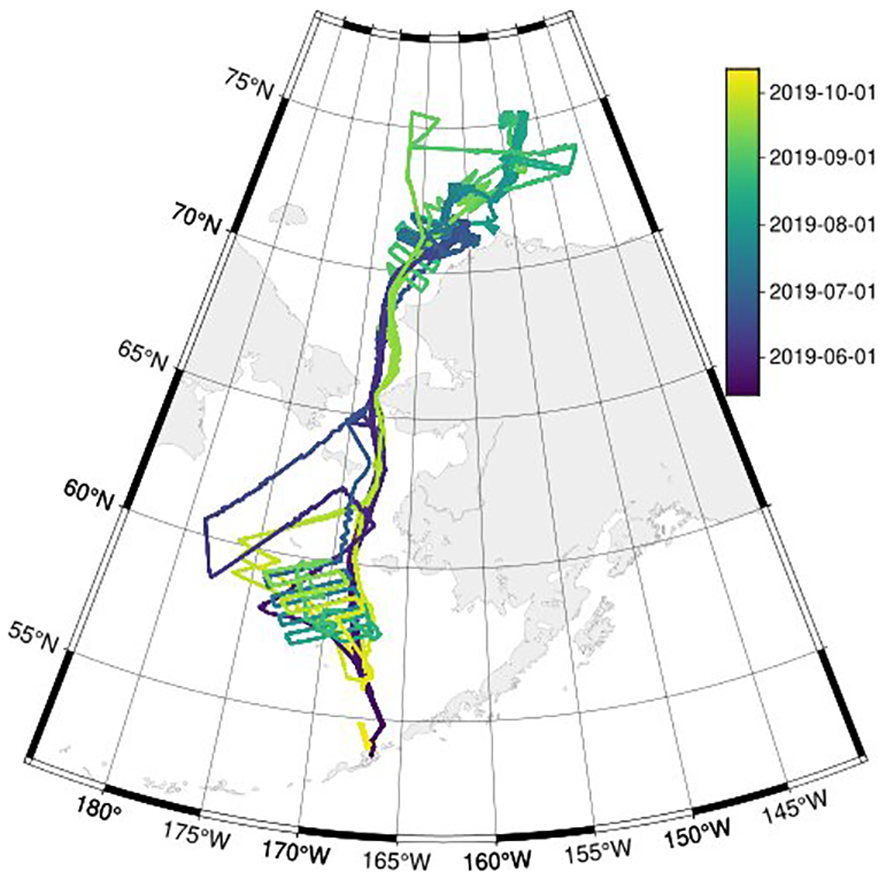
Saildrone tracks during May – October 2019. Colors show the corresponding time of saildrone locations during the deployment period.
Bulk formulas are used to calculate sea surface sensible (QS) and latent (QL) heat fluxes. The Coupled Ocean-Atmosphere Response Experiment (COARE) bulk algorithm version 3.6 (Fairall et al., 2003), updated to account for high wind speed conditions (Edson et al., 2013) and sea ice presence (Andreas, 1987), was applied to saildrone measurements. These flux calculations are represented by Equations 1, 2:
where is the density of surface air and is the 10-meter wind speed. In Equation 1, is the exchange coefficient for sensible heat, the specific heat capacity of air, and the surface water and air temperature, respectively. In Equation 2, is the latent heat of evaporation, and is the exchange coefficient for latent heat. and are the surface saturation and air humidities, respectively. Information regarding the state variables measured by saildrones which are required for calculating fluxes in Equations 1, 2 are listed in Table 1.
Table 1
| Variable | Model | Saildrone | |
|---|---|---|---|
| Vertical level | Height | Instrument | |
| Analysis and 6-hour forecast variables | |||
| Relative Humidity | 2 m | 2.3 m | Rotronic HC2-S3 |
| Temperature | Surface | -0.53 m | RBR Saildrone3 CTD/ODO/Chl-A |
| Temperature | 2 m | 2.3 m | Rotronic HC2-S3 |
| Pressure | Surface | 0.2 m | Vaisala PTB210 |
| Wind Speed | 10 m | 5 m | Gill Anemometer 1590-PK-020 |
| 0–6 hour average variables | |||
| Sensible Heat Flux | Surface | Calculated with COARE | |
| Latent Heat Flux | Surface | Calculated with COARE | |
Forecast variables and related saildrone measurements.
2.2 Global Forecast System models
We examine both deterministic and probabilistic operational forecasts during the 2019 Arctic Saildrone Mission. Surface flux predictions from deterministic forecasts of the NOAA Global Forecast System (GFS) NCEP (2019a) and ensemble forecasts of the Global Earth Forecast System (GEFS) NCEP (2019b) are evaluated against those based on saildrone observations. Information about the two forecasts is given in Table 2.
Table 2
| Model | GFS (Deterministic) | GEFS (Ensemble) |
|---|---|---|
| Version | 14, 15.1* | 11.0 |
| Resolution | 0.25° x 0.25° | 1° x 1° |
| Forecast Length | 0–240 hours (10 days) | 0–384 hours (16 days) |
| Daily Frequency | 6 hours (00, 06, 12, 18 UTC) | 6 hours (00, 06, 12, 18 UTC) |
| Ensemble Members | N/A | 21 members |
Comparison of GFS and GEFS models.
*GFS implemented version 15.1 beginning with the forecast initialized at 06-12–2019 T12:00 UTC.
The Noah Land-Surface Model (Noah-LSM) used in the GFS and GEFS models drives the parametrization of the meteorological state variables used in this study and is primarily responsible for the accuracy of the surface and near-surface forecasts (Ek et al., 2003). Sensible and latent heat fluxes in GFS and GEFS are calculated in the GFS Surface Layer Scheme using the Monin-Obukhov similarity profile relationship based on the framework of Miyakoda and Sirutis (1986) and modifications for stability regimes of Long (1984, 1986). GEFSv11 implements a persistent + relaxation surface temperature parametrization, differing from the more complex Near Sea-Surface Temperature (NSST) Analysis used in GFSv14 and GFSv15.1. The update from GFSv14 to GFSv15.1 changes the dynamical core and some of the microphysics representations in the GFS model. This change and the implementation of the updated GFS version as boundary conditions in GEFSv11 on 10-09–2019 causes discontinuity in the underlying processes which create the fluxes and, thus, distributions of error values. To maintain consistent properties in the flux error data generation, evaluations of fluxes which aggregate observations are only conducted on subsets of the time series with continuous model versions. Surface state variables from the forecasts corresponding to those measured by saildrones are given in Table 1 along with the observations.
Saildrone point observations follow the latitude and longitude of their tracks and are irregularly spatially distributed. These observations need to be paired with forecasts on their regular grid points for their direct comparisons. The hourly saildrone observations are paired with GFS and GEFS forecasts at the nearest grid points. With consideration for ergodicity and the differing spatial scales between saildrone measurements and forecasts applied to grid cell region, saildrone observations are averaged over one hour centered at the forecast time for the state variables and averaged over the 6-hour forecast intervals (Table 1) for flux variables (e.g. as in (Sivam et al., 2024)). Surface and 2-meter temperatures are paired with those measured by the saildrones to find errors in these state variable forecasts. Values of the wind speed from the forecasts are adjusted using the log-law for conversion to match the saildrone wind measurement height. We define forecast errors as forecasts minus observations.
3 Results
We first present examples of observed and forecasted surface sensible and latent heat fluxes along the track of a saildrone (saildrone 1035). Neither the GFS deterministic forecast nor GEFS ensemble forecast (Figure 2) effectively predicts surface sensible and latent heat fluxes with precision or accuracy. Errors in ensemble predictions occasionally exhibit large spikes not seen in the deterministic forecast, as observed in the errors from saildrone 1033 in Figure 3. Some of these error spikes may be attributed to the presence of land cover in the one-degree grid cell of GEFS which is not within the same quarter-degree grid cell of GFS (e.g. spikes in August). Other spikes occur in gid cells which do not contain land (e.g. spikes in June). Through the majority of the time series of saildrone observations, forecasted fluxes are of the wrong signs. This is particularly prevalent when observing sensible heat flux for which the opposite signs of prediction and observation are most often seen not just in the deterministic forecast and ensemble mean, but also each ensemble member. While observed fluxes are mostly positive (energy from the ocean to the atmosphere), forecasted fluxes are negative (energy from the atmosphere to the ocean). Such errors exist even at the very beginning of the forecasts (the average from 0–6 hours).
Figure 2
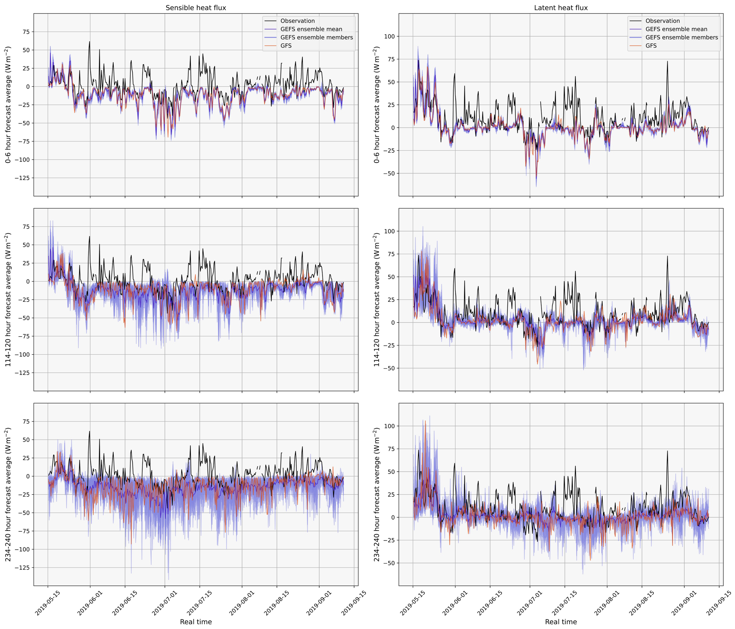
Time series of sensible heat fluxes (left column) and latent heat fluxes (right column) from observations (black), GFS deterministic forecast (orange), and GEFS ensemble means and members (blue) at lead times of 0–6 hours (top row), 114–120 hours (middle), and 234–240 hours (bottom) along the track of saildrone 1035.
Figure 3
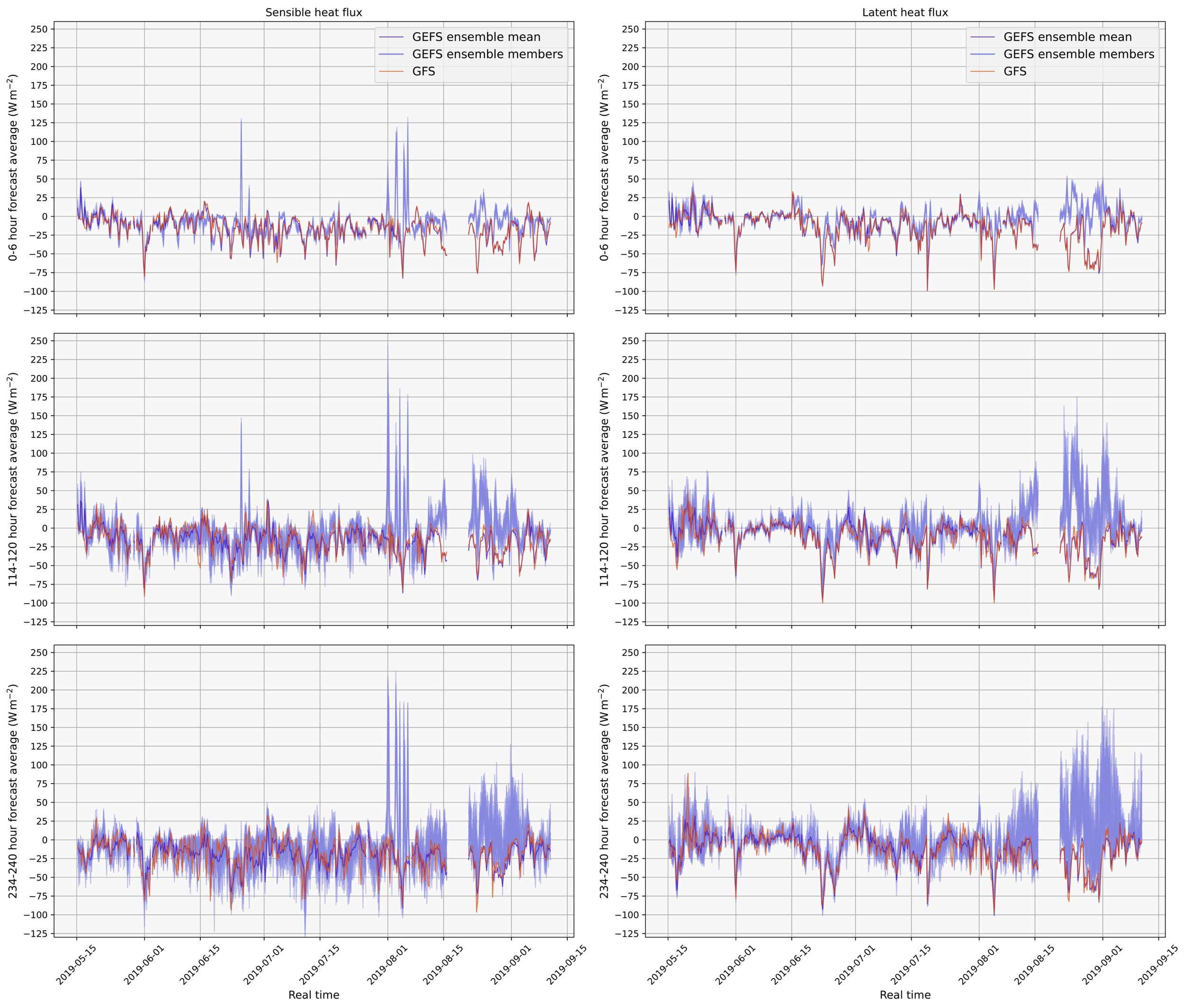
Time series of sensible heat flux (left column) and latent heat flux (right column) errors as predicted - observed from GFS deterministic forecast (orange) and GEFS ensemble means and members (blue) at lead times of 0–6 hours (top row), 114–120 hours (middle), and 234–240 hours (bottom) along the track of saildrone 1033.
Incorrect air-sea differences in temperature and humidity are the largest factors contributing to errors in the signs of the fluxes. The observed and modeled temperatures and humidities at their initial times along the saildrone 1035 track are shown in Figure 4. The differences between modeled and observed surface air temperature () at their initial times are comparable, but there are evident low biases in sea surface temperature () in the models, as seen in Figure 4; Table 3. These biases lead to errors in air-sea temperature differences . In observations, , corresponds with upward (from the ocean to atmosphere) sensible heat fluxes. In contrast, as seen in the models, leads to downward (from the atmosphere to ocean) sensible heat fluxes as seen in Figure 2. Because the surface saturation humidity is determined by , the low bias in leads to low biases in . Consequently, air-sea differences in humidity often have the wrong sign as well, . This leads to negative or downward (from the atmosphere to ocean) latent heat fluxes. A slight low bias is seen in . Given that the differences between observed and modeled are larger than the differences in , this error may be caused by errors in relative humidity forecasts, seen in persistent low bias in Figure 4; Table 3. For errors involvingopposite signs in sensible heat flux prediction and saildrone observation, 90.6% of GFS and 87.0% of GEFS values also had opposite signs between observation and forecast of . For latent heat flux errors, these percentages are 63.5% for GFS and 63.6% for GEFS. Wind speed is also used in the flux calculations, but exhibits no persistent biases, as seen in Table 3, though there is heteroskedastic growth in error as a function of lead time.
Figure 4
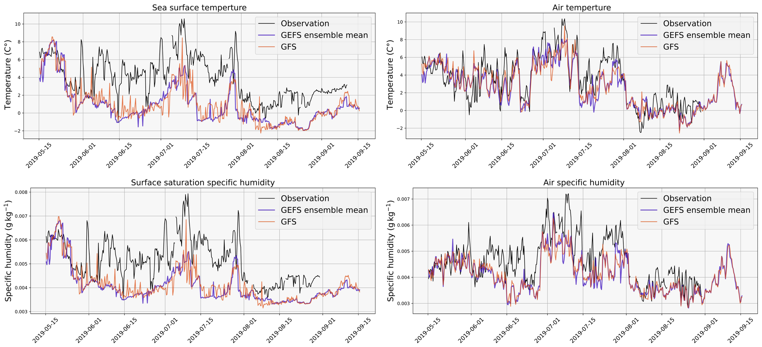
Forecasts of state variables at 0–6 forecast hour for measurements (black), GFS deterministic forecast (orange), and GEFS ensemble mean (blue) along the track of saildrone 1035.
Table 3
| State variables | |||||||||
|---|---|---|---|---|---|---|---|---|---|
| Lead time | Deterministic | Ensemble members | Ensemble mean | ||||||
| RH | Bias | RMSE | Bias | RMSE | Bias | RMSE | |||
| T06 | -7.44 | 11.08 | 0.53 | -8.25 | 11.51 | 0.52 | -8.25 | 11.39 | 0.53 |
| T120 | -7.24 | 11.25 | 0.39 | -9.70 | 13.08 | 0.37 | -9.70 | 12.25 | 0.44 |
| T240 | -7.31 | 12.08 | 0.22 | -9.90 | 13.88 | 0.21 | -9.90 | 12.27 | 0.32 |
| SST | Bias | RMSE | Bias | RMSE | Bias | RMSE | |||
| T06 | -2.45 | 3.02 | 0.90 | -2.54 | 3.13 | 0.90 | -2.54 | 3.13 | 0.90 |
| T120 | -2.91 | 3.55 | 0.87 | -2.91 | 3.55 | 0.88 | -2.91 | 3.55 | 0.88 |
| T240 | -3.24 | 3.97 | 0.84 | -3.21 | 3.94 | 0.85 | -3.21 | 3.93 | 0.85 |
| T2M | Bias | RMSE | Bias | RMSE | Bias | RMSE | |||
| T06 | -0.70 | 1.40 | 0.94 | -0.67 | 1.50 | 0.93 | -0.67 | 1.48 | 0.93 |
| T120 | -1.60 | 2.49 | 0.87 | -1.21 | 2.25 | 0.87 | -1.21 | 2.11 | 0.89 |
| T240 | -1.66 | 2.95 | 0.78 | -1.30 | 2.67 | 0.79 | -1.30 | 2.34 | 0.85 |
| SP | Bias | RMSE | Bias | RMSE | Bias | RMSE | |||
| T06 | -0.33 | 0.76 | 1.00 | -0.31 | 0.98 | 0.99 | -0.31 | 0.89 | 1.00 |
| T120 | 0.44 | 4.48 | 0.87 | 0.14 | 5.16 | 0.83 | 0.14 | 4.14 | 0.88 |
| T240 | -0.37 | 9.62 | 0.40 | -0.36 | 9.77 | 0.36 | -0.36 | 7.54 | 0.53 |
| WSP | Bias | RMSE | Bias | RMSE | Bias | RMSE | |||
| T06 | -0.28 | 1.51 | 0.85 | -0.35 | 1.55 | 0.84 | -0.35 | 1.47 | 0.86 |
| T120 | 0.01 | 3.11 | 0.37 | -0.00 | 3.21 | 0.34 | -0.00 | 2.61 | 0.45 |
| T240 | 0.01 | 3.65 | 0.11 | -0.04 | 3.74 | 0.07 | -0.04 | 2.81 | 0.17 |
| Flux variables | |||||||||
|---|---|---|---|---|---|---|---|---|---|
| Deterministic | Ensemble members | Ensemble mean | |||||||
| QS | Bias | RMSE | Bias | RMSE | Bias | RMSE | |||
| T00–T06 | -11.97 | 17.32 | 0.78 | -12.66 | 18.76 | 0.68 | -12.66 | 18.58 | 0.69 |
| T114–T120 | -9.43 | 20.10 | 0.56 | -11.09 | 22.44 | 0.48 | -11.09 | 20.09 | 0.54 |
| T234–T240 | -10.18 | 25.21 | 0.32 | -13.06 | 27.03 | 0.31 | -13.06 | 22.52 | 0.42 |
| QL | Bias | RMSE | Bias | RMSE | Bias | RMSE | |||
| T00–T06 | -4.77 | 17.07 | 0.74 | -4.95 | 17.52 | 0.69 | -4.95 | 17.31 | 0.69 |
| T114–T120 | -0.09 | 24.36 | 0.59 | -0.46 | 25.41 | 0.53 | -0.46 | 23.02 | 0.57 |
| T234–T240 | -2.09 | 25.61 | 0.41 | -2.11 | 25.46 | 0.39 | -2.11 | 19.64 | 0.50 |
Statistics for GFSv15.1 and GEFSv11 errors along all saildrone tracks.
While errors in the state variables in Equations 1, 2 are correlated with flux errors, the values of , , , , , and themselves are all uncorrelated with the flux errors. Figure 4 shows plots of temperature errors at the averaged 0–6 hour lead time at all saildrone observations, normalized by locations and smoothed with a Gaussian filter to emphasize regions where error is greatest. There is clustering in error direction in both surface and 2-meter temperatures. Particularly large negative surface errors often occur at northern latitudes and some areas within the Bering Sea, though a widespread cold bias is seen. 2-meter temperature errors show more dispersed error signs with smaller absolute error. Overly warm 2-meter temperatures are predicted through most of the Bering Strait.
Temperature errors have strong relationships with flux errors, particularly sensible heat flux errors, as is seen by comparing Figure 5 with Figure 6. The flux errors exhibit spatial clustering, though it does not fully mirror that of temperature errors. Latent heat flux has a greater number of extreme value errors, as seen in Figure 6, which increases the root mean squared error of forecast errors (Table 3).
Figure 5
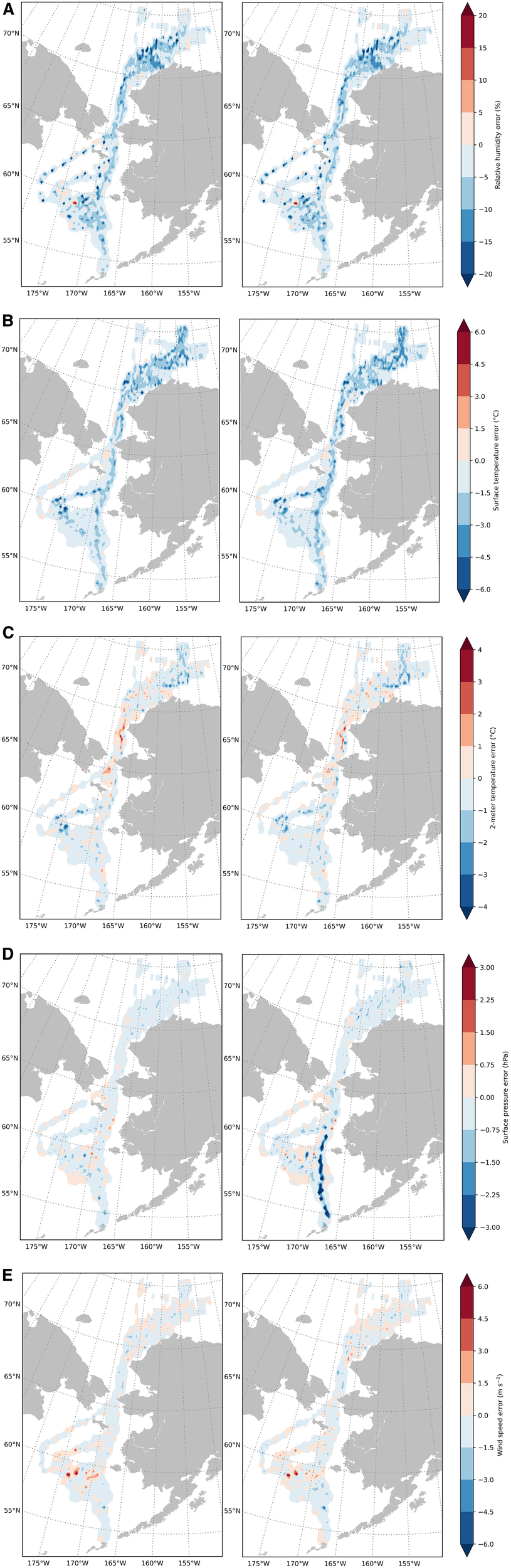
Plots of smoothed forecast errors for all saildrone observations normalized by density for deterministic (left) and ensemble mean (right) (A) relative humidity, (B) surface temperature, (C) 2-meter air temperature, (D) surface pressure, and (E) wind speed at the 0–6 hour averaged lead time.
Figure 6
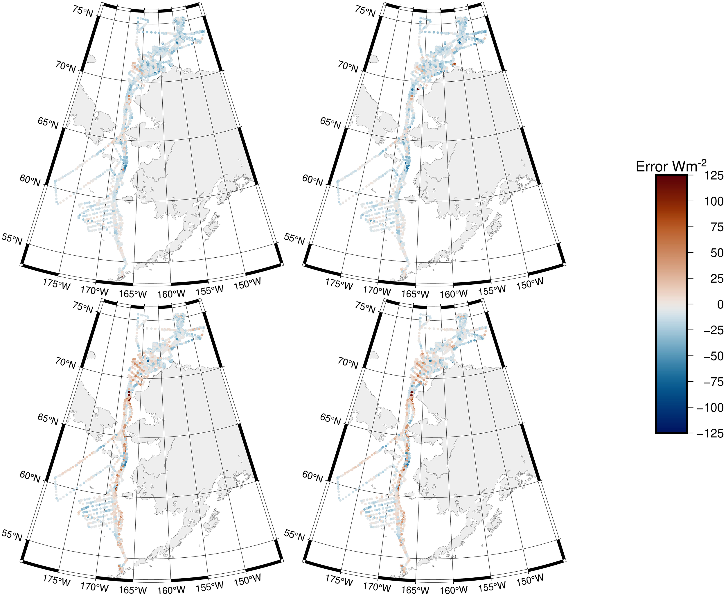
Forecast error along saildrone tracks for QS in GFS (top left), QS in GEFS (top right), QL in GFS (bottom left), and QL in GEFS (bottom right) at the 0–6 hour average lead time.
The growth of the forecast errors (Figure 7) is the fastest from lead times of 2–5 days and gradually slows down beyond that. The GEFS ensemble forecast errors appear to approach their saturation where they are no longer increasing with lead time toward day 15. It is surprising that the GFS deterministic forecasts of sensible heat fluxes outperform the GEFS ensemble forecasts up to the lead time of 10 days (Figure 7). The out performance of deterministic forecast over ensemble mean is seen as well for latent heat fluxes (Figure 7) up to day 6, but the differences are much smaller than for sensible heat fluxes. This casts a doubt that model resolution (higher in GFS than GEFS) is a viable explanation for the outperformance of the GFS deterministic forecasts of sensible heat fluxes. Figure 5 shows that there are more local errors in surface pressure for the ensemble forecast which could contribute to the outperformance of the deterministic model for latent heat fluxes. Possible differences in the parameterization schemes of sensible heat fluxes and atmospheric boundary layer in the two forecast models need to be explored to further explain the forecast error differences.
Figure 7
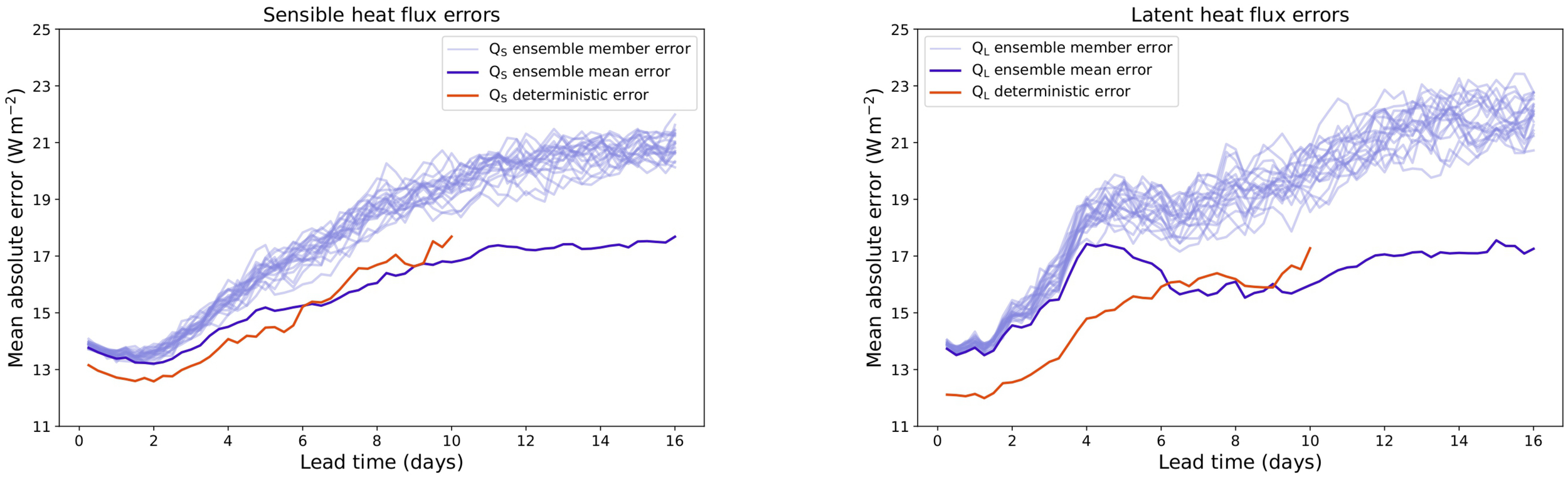
Growth of absolute errors for GFSv15.1 and GEFSv11 forecasts of sensible (left) and latent (right) heat fluxes with lead time.
Correlations between the observations and forecasts (Figure 8) confirm the result from Figure 7 that the GFS deterministic forecasts (dots) outperform the GEFS ensemble forecasts (lines) up to lead time of 6 days. As expected, ensemble means (solid lines) outperform ensemble members (dashed). In all cases, the correlation coefficients quickly decrease during the first week of the forecasts.
Figure 8
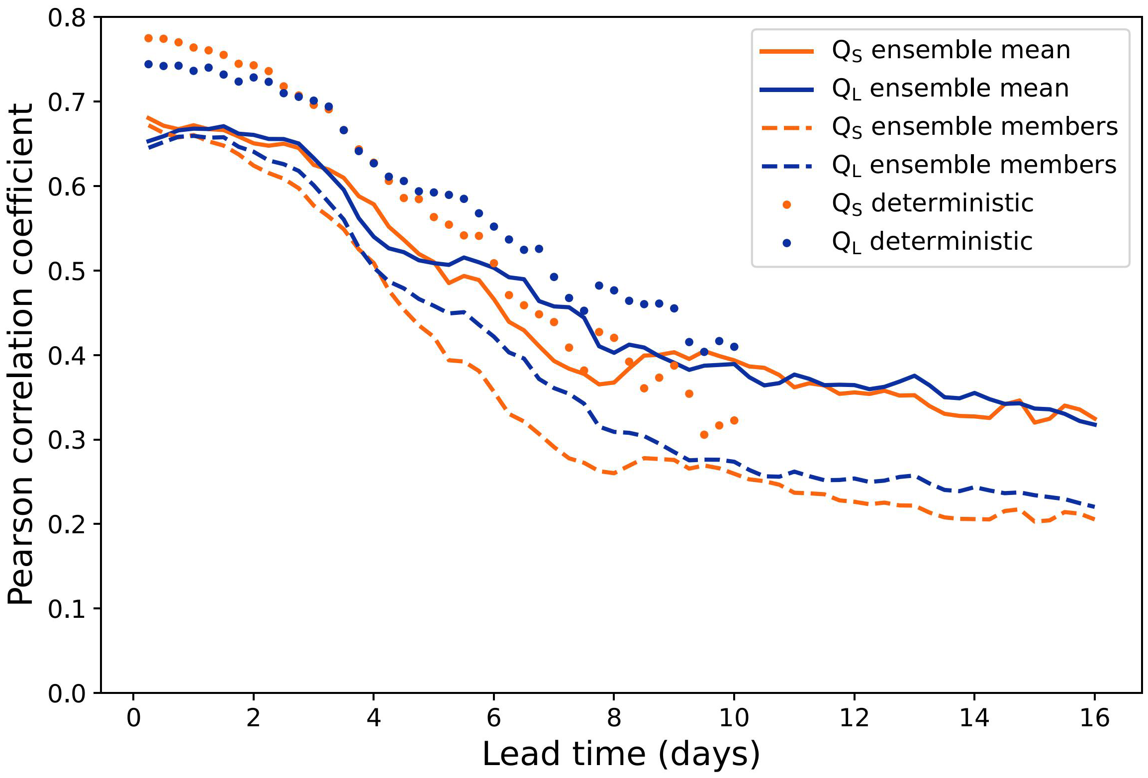
Pearson correlation coefficient between GFSv15.1 and GEFSv11 forecasted and observed fluxes at different lead times.
4 Conclusions
In this study, observations from six uncrewed surface vehicles, saildrones, deployed in the Arctic during May – October 2019 are used to validate surface sensible and latent heat fluxes in two forecast systems: GFS deterministic forecast and GEFS ensemble forecasts. To the best of our knowledge, this is the first time observations from uncrewed surface vehicles are used to validate forecasts of surface fluxes.
Comparisons between the observed and forecasted surface fluxes reveal two unexpected results. First, there are evident low biases in sea surface temperature (SST) in the initial conditions of both forecast systems. The low biases in SST lead to negative air-sea differences in temperature and humidity (sea surface values minus surface air values). Consequently, surface sensible and latent heat fluxes in the forecast are driven toward negative fluxes (from the atmosphere into ocean) during times in which surface fluxes calculated from observations are positive (from the ocean to atmosphere). Second, it is found that the GFS deterministic forecasts outperform the GEFS ensemble forecast for the first 6 days, particularly in surface sensible heat fluxes. The reason for this remains unclear and needs to be explored by examining the detailed differences between the parameterization schemes used by the two forecast models.
Much of the error is likely attributed to temperature errors, particularly sea surface temperature. Some error could be created by transfer coefficients in the flux calculations, differences between algorithm parameterizations, such as roughness lengths and stability terms (e.g. Vickers and Mahrt (2006); Brunke et al. (2006)). Since values of state variables are uncorrelated with flux errors, it is unlikely that errors in predicted fluxes are associated with global meteorology trends. Instead, clusters in sign and magnitude of error show regional patterns, as seen in Figures 5, 6. There is spatial correlation between errors in surface and air temperatures in clusters throughout the study region, supporting that these errors are caused by model misrepresentations that can be widespread, such as clouds, rather than region-specific errors (e.g. sea ice). More robust spatial analysis is needed to evaluate the local processes which could create these errors.
This study supports the feasibility of using limited in situ observations from uncrewed observing systems to uncover unambiguous forecast errors, and encourages similar validation to be performed with forecasts by model prediction systems. The updates to the deterministic forecast which were implemented during this study period created major changes to the algorithm which calculates fluxes, including the FV3 dynamical core which is used in current model versions. It is discouraging that despite these updates, the signs of surface sensible and latent heat fluxes are very often incorrect, despite their crucial role in the Arctic energy balance. Despite any improvement in forecast error, the deterministic forecast typically follows the opposing sign trends of the ensemble forecast which does not include these updates.
This study signifies the need for in situ observations for variables that cannot be reliably retrieved from satellites, in regions such as the Arctic, for correct forecast initial conditions. In this case, the use of in situ observations of sea surface temperature to inform forecast initial conditions could greatly reduce errors in the forecast of surface sensible and latent heat fluxes. The new observing technologies of uncrewed systems have begun to remedy the long-lasting lack of in situ observations over the Arctic open ocean. There is a critical need for a global strategy to optimize the potential of uncrewed observing systems given the minimal resources required for their use and their potential to improve forecasts. The development of such a strategy is currently underway (Patterson et al., 2025).
Statements
Data availability statement
The datasets analyzed for this study can be found in the NCEP GFS 0.25 Degree Global Forecast Grids Historical Archive https://rda.ucar.edu/datasets/d084001/, the AWS NOAA Global Ensemble Forecast System (GEFS) archive https://registry.opendata.aws/noaa-gefs/, and the Pacific Marine Environmental Laboratory’s ERDDAP data server for public access to scientific data https://data.pmel.noaa.gov/pmel/erddap/tabledap/index.html.
Author contributions
HH: Writing – original draft, Writing – review & editing, Data curation, Formal analysis, Methodology, Software, Visualization. CZ: Writing – review & editing, Data curation, Methodology, Conceptualization, Project administration, Resources, Supervision. DZ: Writing – review & editing, Data curation, Formal analysis. HMH: Writing – review & editing, Funding acquisition, Supervision.
Funding
The author(s) declared that financial support was received for this work and/or its publication. This study is supported by the NOAA William M. Lapenta Student Internship Program (HH), and other grants.
Acknowledgments
This is PMEL contribution number 5723.
Conflict of interest
The author(s) declared that this work was conducted in the absence of any commercial or financial relationships that could be construed as a potential conflict of interest.
Generative AI statement
The author(s) declared that generative AI was not used in the creation of this manuscript.
Any alternative text (alt text) provided alongside figures in this article has been generated by Frontiers with the support of artificial intelligence and reasonable efforts have been made to ensure accuracy, including review by the authors wherever possible. If you identify any issues, please contact us.
Publisher’s note
All claims expressed in this article are solely those of the authors and do not necessarily represent those of their affiliated organizations, or those of the publisher, the editors and the reviewers. Any product that may be evaluated in this article, or claim that may be made by its manufacturer, is not guaranteed or endorsed by the publisher.
References
1
Andreas E. L. (1987). A theory for the scalar roughness and the scalar transfer coefficients over snow and sea ice. Boundary-Layer Meteorology38, 159–184. doi: 10.1007/BF00121562
2
Brunke M. A. Zhou M. Zeng X. Andreas E. L. (2006). An intercomparison of bulk aerodynamic algorithms used over sea ice with data from the surface heat budget for the arctic ocean (sheba) experiment. J. Geophysical Research: Oceans111. doi: 10.1029/2005JC002907
3
Chiodi A. M. Zhang C. Cokelet E. D. Yang Q. Mordy C. W. Gentemann C. L. et al . (2021). Exploring the pacific arctic seasonal ice zone with saildrone usvs. Front. Mar. Sci.8. doi: 10.3389/fmars.2021.640697
4
Cokelet E. D. Meinig C. Lawrence-Slavas N. Stabeno P. J. Mordy C. W. Tabisola H. M. et al . (2015). “ The use of saildrones to examine spring conditions in the bering sea,” in OCEANS 2015-MTS/IEEE Washington. 1–7 ( IEEE). doi: 10.23919/OCEANS.2015.7404357
5
Dai A. Jenkins M. T. (2023). Relationships among arctic warming, sea-ice loss, stability, lapse rate feedback, and arctic amplification. Climate Dynamics61, 5217–5232. doi: 10.1175/BAMS-D-20-0086.1
6
Dai H. (2021). Roles of surface albedo, surface temperature and carbon dioxide in the seasonal variation of arctic amplification. Geophysical Res. Lett.48, e2020GL090301. doi: 10.1029/2020GL090301
7
Edson J. B. Jampana V. Weller R. A. Bigorre S. P. Plueddemann A. J. Fairall C. W. et al . (2013). On the exchange of momentum over the open ocean. J. Phys. Oceanography43, 1589–1610. doi: 10.1175/JPO-D-12-0173.1
8
Ek M. B. Mitchell K. E. Lin Y. Rogers E. Grunmann P. Koren V. et al . (2003). Implementation of noah land surface model advances in the national centers for environmental prediction operational mesoscale eta model. J. Geophys. Res.108, 8851. doi: 10.1029/2002JD003296
9
Fairall C. W. Bradley E. F. Hare J. E. Grachev A. A. Edson J. B. (2003). Bulk parameterization of air–sea fluxes: Updates and verification for the coare algorithm. J. Climate16, 571–591. doi: 10.1175/1520-0442(2003)016⟨0571:BPOASF⟩2.0.CO;2
10
Gultepe I. Sharman R. Williams P. D. Zhou B. Ellrod G. Minnis P. et al . (2019). A review of high impact weather for aviation meteorology. Pure Appl. geophysics176, 1869–1921. doi: 10.1007/s00024-019-02168-6
11
Kug J.-S. Jeong J.-H. Jang Y.-S. Kim B.-M. Folland C. K. Min S.-K. et al . (2015). Two distinct influences of arctic warming on cold winters over north america and east asia. Nat. Geosci.8, 759–762. doi: 10.1038/ngeo2517
12
Long P. J. (1984). A General Unified Similarity Theory for the Calculation of Turbulent Fluxes in the Numerical Weather Prediction Models for Unstable Condition ( Office Note 302, U.S. Department of Commerce, National Oceanic and Atmospheric Administration, National Weather Service, National Meteorological Center).
13
Long P. J. (1986). An Economical and Compatible Scheme for Parameterizing the Stable Surface Layer in the Medium-Range Forecast Model ( Office Note 321, U.S. Department of Commerce, National Oceanic and Atmospheric Administration, National Weather Service, National Meteorological Center).
14
Meinig C. Burger E. F. Cohen N. Cokelet E. D. Cronin M. F. Cross J. N. et al . (2019). Public–private partnerships to advance regional ocean-observing capabilities: a saildrone and noaa-pmel case study and future considerations to expand to global scale observing. Front. Mar. Sci.6, 448. doi: 10.3389/fmars.2019.00448
15
Meinig C. Lawrence-Slavas N. Jenkins R. Tabisola H. M. (2015). “ The use of saildrones to examine spring conditions in the bering sea: Vehicle specification and mission performance,” in OCEANS 2015-MTS/IEEE Washington. 1–6 ( IEEE). doi: 10.23919/OCEANS.2015.7404348
16
Miyakoda K. Sirutis J. (1986). Manual of the e-physics Vol. 97 ( Princeton University).
17
NASA/JPL (2019). Saildrone Arctic field campaign surface and ADCP measurements for NOPP-MISST project. (CA, USA: PO.DAAC) doi: 10.5067/SDRON-NOPP0
18
NCEP (2019a). NCEP GFS 0.25 Degree Global Forecast Grids Historical Archive. ( NSF National Center for Atmospheric Research)
19
NCEP (2019b). NOAA Global Ensemble Forecast System (GEFS). Available online at: https://registry.opendata.aws/noaa-gefs
20
Ormevik A. B. Fagerholt K. Meisel F. Sandvik E. (2023). A high-fidelity approach to modeling weather-dependent fuel consumption on ship routes with speed optimization. Maritime Transport Res.5, 100096. doi: 10.1016/j.martra.2023.100096
21
Overland J. E. Wood K. R. Wang M. (2011). Warm arctic—cold continents: climate impacts of the newly open arctic sea. Polar Res.30, 15787. doi: 10.3402/polar.v30i0.15787
22
Patterson R. G. Cronin M. F. Swart S. Beja J. Edholm J. M. McKenna J. et al . (2025). Uncrewed surface vehicles in the global ocean observing system: a new frontier for observing and monitoring at the air-sea interface. Front. Mar. Sci.12, 1523585. doi: 10.3389/fmars.2025.1523585
23
Rantanen M. Karpechko A. Y. Lipponen A. Nordling K. Hyvärinen O. Ruosteenoja K. et al . (2022). The arctic has warmed nearly four times faster than the globe since 1979. Commun. Earth Environ.3, 168. doi: 10.1038/s43247-022-00498-3
24
Serreze M. C. Barrett A. Stroeve J. Kindig D. Holland M. (2009). The emergence of surface-based arctic amplification. cryosphere3, 11–19. doi: 10.5194/tc-3-11-2009,2009
25
Sivam S. Zhang C. Zhang D. Yu L. Dressel I. (2024). Surface latent and sensible heat fluxes over the pacific sub-arctic ocean from saildrone observations and three global reanalysis products. Front. Mar. Sci.11, 1431718. doi: 10.3389/fmars.2024.1431718
26
Vickers D. Mahrt L. (2006). Evaluation of the air-sea bulk formula and sea-surface temperature variability from observations. J. Geophysical Research: Oceans111. doi: 10.1029/2005JC003323
27
Walsh J. E. (2014). Intensified warming of the arctic: Causes and impacts on middle latitudes. Global Planetary Change117, 52–63. doi: 10.1016/j.gloplacha.2014.03.003
28
Yamanouchi T. Takata K. (2020). Rapid change of the arctic climate system and its global influences overview of grene arctic climate change research project, (2011–2016). Polar Sci.25, 100548. doi: 10.1016/j.polar.2020.100548
29
Zhang D. Cronin M. F. Meinig C. Farrar J. T. Jenkins R. Peacock D. et al . (2019). Comparing air-sea flux measurements from a new unmanned surface vehicle and proven platforms during the spurs-2 field campaign. Oceanography32, 122–133. doi: 10.5670/oceanog.2019.220
30
Zhang C. Levine A. F. Wang M. Gentemann C. Mordy C. W. Cokelet E. D. et al . (2022). Evaluation of surface conditions from operational forecasts using in situ saildrone observations in the pacific arctic. Monthly Weather Rev.150, 1437–1455. doi: 10.1175/MWR-D-20-0379.1
Summary
Keywords
Arctic ocean, forecast validation, in situ observations, latent and sensible heat flux, saildrone
Citation
Hunter H, Zhang C, Zhang D and Horowitz HM (2026) Validation of forecasted surface sensible and latent heat fluxes by GFS and GEFS against saildrone observations in the Arctic. Front. Mar. Sci. 13:1572290. doi: 10.3389/fmars.2026.1572290
Received
06 February 2025
Revised
29 December 2025
Accepted
05 January 2026
Published
02 February 2026
Volume
13 - 2026
Edited by
Junde Li, Hohai University, China
Reviewed by
Hiroyuki Tomita, Hokkaido University, Japan
Shui Yu, Chinese Academy of Sciences (CAS), China
Updates
Copyright
© 2026 Hunter, Zhang, Zhang and Horowitz.
This is an open-access article distributed under the terms of the Creative Commons Attribution License (CC BY). The use, distribution or reproduction in other forums is permitted, provided the original author(s) and the copyright owner(s) are credited and that the original publication in this journal is cited, in accordance with accepted academic practice. No use, distribution or reproduction is permitted which does not comply with these terms.
*Correspondence: Hope Hunter, hhunter3@illinois.edu
Disclaimer
All claims expressed in this article are solely those of the authors and do not necessarily represent those of their affiliated organizations, or those of the publisher, the editors and the reviewers. Any product that may be evaluated in this article or claim that may be made by its manufacturer is not guaranteed or endorsed by the publisher.