Abstract
The accelerated decline of Arctic sea ice is profoundly reshaping regional climate regimes. Sea ice thickness (SIT), particularly under thin-ice conditions, is an important indicator for assessing early-season Arctic sea ice variability, and accurate prediction of its spatiotemporal evolution during the early freezing period is essential for characterizing short-term sea ice changes. In recent years, deep learning has emerged as a complementary approach to traditional sea ice prediction methods. However, existing deep learning-based studies have not fully exploited the large-scale spatial patterns and temporal contextual dependencies inherent in satellite-derived sea ice thickness. To address this limitation, this study proposes a spatiotemporal prediction framework named EOF-Trans for predicting daily-scale variability of thin sea ice thickness during the early freezing season. The method employs Empirical Orthogonal Functions (EOF) to decompose the sea ice thickness field into temporal mode series, utilizes a Transformer architecture to learn the temporal evolution characteristics, and subsequently reconstructs the predicted outputs back into the spatial thickness field by EOF, thereby enabling spatiotemporal sea ice prediction up to a leadtime of 21 days. Experimental results in the Beaufort Sea indicate that the proposed EOF-Trans framework significantly outperforms numerical models and classical deep learning architectures such as U-Net and ConvLSTM. On the 2022–2023 test set, it achieves a correlation coefficient of 88.04%, representing a 2% improvement over U-Net. Even at a leadtime of 21 days, the correlation remains approximately 84%, with the maximum spatial bias not exceeding 0.5 m. These results indicate that EOF-Trans effectively captures spatiotemporal regularities present in thin sea ice thickness, providing a complementary data-driven perspective for short-term sea ice prediction during the early freezing season.
1 Introduction
With global warming accelerating the melting of Arctic sea ice, multi-year ice is increasingly transforming into first-year ice (Lindsay and Zhang, 2005), and the average thickness of sea ice has decreased by 20% compared to 2010 (Laxon et al., 2013). The sharp reduction in sea ice thickness presents potential opportunities for opening Arctic shipping routes and conducting scientific research activities (Huntington et al., 2015). However, the rapid changes in sea ice thickness over time and space also impose higher demands on the accuracy of current spatiotemporal prediction models for sea ice thickness. Therefore, accurate spatiotemporal prediction of Arctic sea ice thickness has become one of the important issues for ensuring human activities in the Arctic region.
The research on sea ice prediction is witnessing a profound transformation from traditional approaches to a data-driven paradigm. Sea ice prediction based on numerical models was first proposed. These models simulate the thermodynamic and dynamic processes of sea ice evolution, using mathematical equations based on explicit physical laws and given initial-boundary conditions, and provide highly interpretable simulation results (Notz and Bitz, 2017; Guo et al., 2020; Liu et al., 2021). Currently, sea ice prediction models based on numerical models have been widely applied in various forecasting systems, such as the Operational TOPical Ocean and Polar seas model (TOPAZ), the Arctic and Atlantic operational model, and the Canadian Global Ice Ocean Prediction System (GIOPS), playing a significant role in revealing the mechanisms of sea ice spatiotemporal evolution. However, the existing system of physical laws remains incomplete, compelling researchers to simplify the description of sea ice constitutive relations in numerical models. For instance, the single-category assumption for sea ice thickness in the TOPAZ forecasting system cannot finely capture the spatial heterogeneity of sea ice thickness distribution (Sakov et al., 2012). The Arctic and Atlantic operational model refines the hierarchical description of sea ice thickness but remains too coarse in depicting multi-year ice (Madsen et al., 2016). Although GIOPS employs 10 different thickness levels to simulate the evolution of multi-year ice, its neglect of wave–ice interactions hinders further improvement in performance (Smith et al., 2016). Clearly, the simplification of physical processes limits the ability of numerical models to represent the complexly nonlinear relationships in sea ice. Meanwhile, numerical models heavily rely on data assimilation. For example, the Regional Ice Prediction System (RIPS) assimilates sea ice thickness data only at intervals, resulting in a delay in the model simulation of ice thickness (Lemieux et al., 2016). Although the Arctic Ice Ocean Prediction System (ArcIOPS) has achieved some improvement by timely assimilating remote sensing data of sea ice thickness, the simulation results still exhibit significant uncertainty (Mu et al., 2019; Xi et al., 2019). This indicates that the dependence on data assimilation restricts the precision of the model (Wayand et al., 2019). In contrast, deep learning illuminates the intricate laws of dynamic change from a data-centric perspective, freeing itself from the constraints of physical laws that numerical models rely on. This breakthrough paves a new technical avenue for sea ice prediction.
The remarkable achievements (Junhwa and Hyun Cheol, 2021; Durand et al., 2024) of deep learning in polar research suggest that it can serve as a new alternative for sea ice prediction. Deep learning predicts sea ice changes in a data-driven, implicit modeling manner, possessing strong nonlinear relationship fitting capabilities without the need for predefined physical equations (Li et al., 2024). Additionally, it can establish end-to-end relational mappings based on data dependencies, eliminating the reliance on data assimilation (Reichstein et al., 2019). Chi and Kim (2017) were the first to apply deep learning to sea ice concentration prediction, achieving results comparable to numerical models (Chi et al., 2021), but they did not account for the spatiotemporal relationships in sea ice changes. Kim et al. (2020)designed a convolutional neural network to extract spatial features of sea ice concentration but overlooked temporal feature extraction. Feng et al. (2023) and He et al. (2022) introduced the ConvLSTM (Shi et al., 2015) into the field of sea ice prediction, significantly improving forecasting performance. ConvLSTM combines the advantages of convolutional neural networks (Derry et al., 2023) and long short-term memory networks (Hochreiter and Schmidhuber, 1997), using CNN to extract spatial features of sea ice changes and LSTM to establish temporal dependencies, thereby modeling the spatiotemporal evolution of sea ice. Unlike sea ice concentration, sea ice thickness exhibits strong spatial autocorrelation (Ponsoni et al., 2019), which demands higher spatial feature modeling capabilities from the model. However, ConvLSTM, constrained by the size of convolutional kernels, struggles to describe the global features of sea ice spatiotemporal changes. Fortunately, empirical orthogonal functions (EOF) have proven advantageous in capturing spatial features. Yuan et al. (2016) used EOF to characterize the overall covariability of sea ice, and achieve favorable prediction results. Wang et al. (2023) demonstrated the predictability of sea ice thickness through EOF and Markov models.
Inspired by the aforementioned studies, this study proposes a new predictive approach for the spatiotemporal prediction of sea ice thickness, referred to as EOF-Trans. The method employs Empirical Orthogonal Functions to characterize the spatial variability patterns of sea ice thickness, thereby addressing the limitation of existing deep learning models whose convolutional structures are often insufficient for capturing global-scale spatial features. In addition, Transformer architectures are adopted in place of LSTM networks. This choice is motivated by the iterative nature of LSTMs, which constrains their ability to fully represent feature dependencies across different time steps, whereas Transformers (Ashish et al., 2023), through their attention mechanism, are capable of establishing contextual relationships among sea ice thickness patterns across time. EOF-Trans integrates the respective strengths of EOFs and Transformers in spatial and temporal representation learning. Through its SIT spatiotemporal decomposition module, prediction module, and reconstruction module, the proposed method facilitates the prediction of Arctic sea ice thickness in the short term with high accuracy.
2 Materials and methods
2.1 Study site and data
As shown in Figure 1, the Beaufort Sea region in the Arctic (longitude: 135° to 168°W, latitude: 72° to 79°N) was selected as the study area. This study site has a high latitude, and the cold Beaufort Current ensures the presence of extensive annual sea ice and multi-year sea ice in the area (Wiebke et al., 2020; Timmermans and Toole, 2023), which can fully verify the performance of the models.
Figure 1
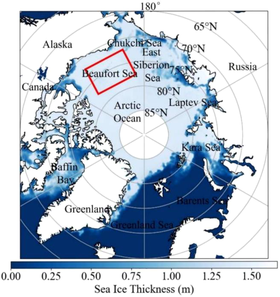
Study site. The base map shows the SMOS L3 SIT data on January 12, 2019 and study site in Beaufort Sea are marked with red box.
The Soil Moisture and Ocean Salinity (SMOS) satellite, launched by the European Space Agency (ESA), carries an L-band two-dimensional synthetic aperture microwave radiometer that is highly sensitive to the emissivity characteristics of sea ice with varying thicknesses. This enables long-term, large-scale, and high-frequency observations of Arctic sea ice thickness (Kaleschke et al., 2012). The SMOS Level 3 Sea Ice Thickness (SMOS L3 SIT) product released by ESA provides both high temporal and high spatial resolution, making it one of the few gridded sea ice thickness datasets that simultaneously offer daily temporal resolution and a spatial resolution of 12.5 km, Table 1. Such characteristics allow the dataset to capture finer-scale temporal variations and spatial patterns of sea ice thickness, which is particularly valuable for the present study.
Table 1
| Dataset name | Temporal resolution | Time span | Spatial resolution | Spatial coverage |
|---|---|---|---|---|
| SMOS L3 (Kaleschke et al., 2012) | Daily | 2010–Present (October–April) | 12.5 km | 50°–90°N |
| CS2SMOS (Ricker et al., 2017) |
Weekly | 2010–Present (October–April) | 25 km | 50°–90°N |
| AWI (Ricker et al., 2014) | Monthly | 2010–Present (October–April) | 25 km | 50°–90°N |
| CPOM (Tilling et al., 2015) | 2/14/28 days | 2010–Present (October–April) | 5 km/1 km interpolated | Above 60°N |
| ESA CCI (Ricker et al., 2025) | Monthly | 2002–2020 (October–April) | 25 km | 50°–90°N |
| IS2SITMOGR4 (Petty et al., 2020) |
Monthly | 2018–Present (November–April) | 25 km | 55°–90°N |
International mainstream gridded sea ice thickness products.
Moreover, the observational accuracy of the SMOS L3 SIT product has been extensively validated and widely recognized (Kaleschke et al., 2016), and it has been successfully applied in various contexts, including data assimilation in numerical models (Xie et al., 2016; Gupta et al., 2021). ESA has been providing daily sea ice thickness observations from SMOS since the 2010 freeze-up season, and the dataset is publicly accessible. In this study, SMOS L3 SIT data from October 15 to January 15 of each year were collected to support the short-term prediction of Arctic sea ice thickness.
3 Methods
Sea ice undergoes rapid, short-term changes, and current deep learning models still struggle to fully exploit the global spatial characteristics of sea ice thickness and lack a focus on important temporal information. To achieve accurate daily-scale prediction of sea ice thickness, EOF-Trans has been proposed. As shown in Figure 2, EOF-Trans consists of three parts: the spatiotemporal decomposition module, the prediction module, and the reconstruction module. The spatiotemporal decomposition module decomposes the spatiotemporal data of sea ice thickness into Orthogonal Spatial Modes (EOFs) and corresponding Principal Components (PCs) to capture the spatial distribution patterns of sea ice thickness in the spatiotemporal domain and their trends over time, Figure 2a. The prediction module uses attention mechanisms to dynamically assign weights to each time step in the sea ice thickness sequence, enabling EOF-Trans to focus on temporal features that affect changes in sea ice thickness, Figure 2b. At the same time, EOF-Trans leverages an encoder-decoder structure to fit the nonlinear temporal changes of sea ice thickness. The reconstruction module then integrates the EOFs from the spatiotemporal decomposition module and the PCs output by the prediction module to reconstruct the sea ice thickness data, yielding the final sea ice thickness forecast results, Figure 2c.
Figure 2
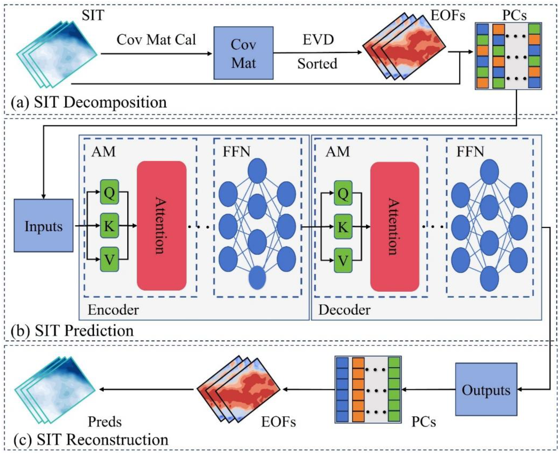
EOF-Trans Workflow. (a) Sea ice thickness decomposition module, (b) sea ice thickness prediction module, and (c) sea ice thickness reconstruction module. In which, Cov Mat Cal denotes the calculation of the covariance matrix, Cov Mat represents the covariance matrix, EVD denotes Eigen Value Decomposition, AM stands for attention mechanism, Q, K, V respectively represent the components of the attention mechanism, namely query, key, value, FFN stands for feed-forward neural network.
3.1 Spatiotemporal decomposition of sea ice thickness
The atmosphere, ocean, and sea ice are interacted and influence each other, making the changes in sea ice thickness not spatially independent. Current research is dedicated to characterizing the local variations of SIT, while the redundancy of observational data in terms of spatial distribution characteristics and temporal trends poses a challenge to the description of the global features of SIT. Spatiotemporal decomposition can decompose the SIT data to identify and separate time and space information, aiding in understanding the intrinsic mechanisms of sea ice thickness and describing its variation characteristics.
As shown in Figure 2a, Empirical Orthogonal Function (EOF) is a spatiotemporal analysis method (Deser et al., 2000) for extracting the main patterns and characteristics from SIT data. It projects the SIT data onto the covariance matrix through covariance matrix calculations and decomposes the time-varying SIT data into time-invariant EOFs and time-dependent PCs through Eigen Value Decomposition (EVD).
Assuming represents the number of SIT spatial points on a given day, and represents the number of time series at a certain location, then the SIT data can be represented as . Eliminating the influence of long-term states in the SIT variations, the SIT anomaly matrix is calculated using Equation 1:
Then can be expressed as Equation 2:
in which, the element represents the SIT data at the -th time point and the -th spatial point.
From , the SIT covariance matrix can be obtained using Equation 3:
Subsequently, through EVD, the SIT spatial eigenvectors and their corresponding time coefficients are obtained using Equation 4:
in which, is a diagonal matrix with the time coefficients arranged in descending order, as in Equation 5:
Ultimately, by matrix multiplication, the time components corresponding to are obtained using Equation 6:
The SIT observation at a specific moment is viewed as a linear combination of various spatial modes with different weights. The spatiotemporal decomposition module decomposes the SIT data into EOFs and PCs. Consequently, the variation in SIT is transformed into spatial modes that do not change with time and different series components containing spatiotemporal information, which aids in describing its underlying mechanisms.
3.2 Spatiotemporal prediction of sea ice thickness
Characterizing the temporal variation characteristics of SIT is essential for obtaining accurate daily-scale spatiotemporal forecasts of SIT, yet current research lacks consideration of contextual features in SIT temporal variation. Compared to other deep learning models, the Transformer can build associations between any two elements in the sequence through attention mechanisms, characterizing the variation characteristics of SIT sequences without being affected by the length of the dataset (Ashish et al., 2023). As shown in Figure 2b, the Transformer is introduced and used to construct contextual features of SIT PCs in the temporal domain. The PCs derived from SIT data are input into the Transformer, and the predicted PCs are obtained through the encoder and decoder.
Figures 3a, b illustrate the Encoder-Decoder architecture of the Transformer. The Encoder is used to generate the contextual representation of the spatiotemporal variation of SIT for the Decoder. The Encoder consists of multiple identical layers, each containing a multi-head attention mechanism and a feed-forward neural network. Each sublayer is followed by residual connections and layer normalization, which helps alleviate the vanishing gradient problem and stabilize model training. The Decoder predicts the PCs for future moments based on the generated SIT contextual representation and SIT PCs. Similarly, the Decoder is composed of multiple identical layers, with the main sublayers including a masked multi-head attention mechanism, a multi-head attention mechanism, and a feed-forward neural network.
Figure 3
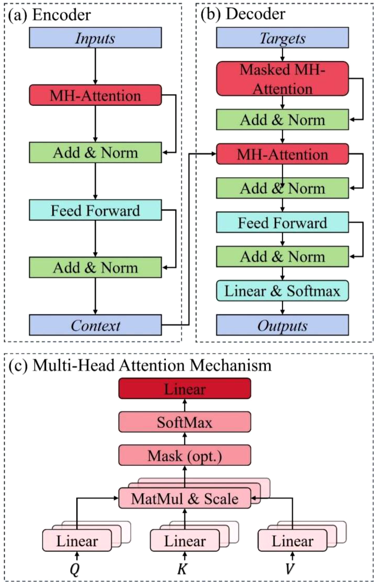
Transformer architecture. (a) Encoder, (b) decoder, and (c) multi-head attention mechanism. In which, Add & Norm represents addition and layer normalization, MatMul & Scale represents matrix multiplication and scaling, Linear & Softmax represents the linear layer and the Softmax function.
Establishing dependencies between different parts of the SIT PCs in the temporal sequence and capturing relationships between different locations rely on the Multi-Head (MH) attention mechanism. Figure 3c shows the MH attention mechanism used, which includes multiple parallel attention mechanisms to capture different features and relationships within the input SIT data, as in Equation 7:
in which, is the weight matrix, and the nth attention mechanism in the cascade, , can be expressed using Equation 8:
in which, is the scaling factor, and the elements of the attention mechanism, query , key , and value , are obtained by passing the SIT PCs through three distinct linear transformation layers.
Therefore, when using the Transformer for spatiotemporal prediction of SIT, the SIT PCs with positional encoding are input into the encoder, as in Equation 9:
focuses on the important locations of the SIT PCs input by exploring the complex dependencies between different positions, thereby generating a contextual representation of the sea ice sequence, as in Equation 10:
The feed-forward neural network applies non-linear transformations to , enhancing the expressive power of Transformer over SIT PCs, as shown in Equation 11:
In the decoder, Masked Multi-Head (MMH) attention is used to gather contextual information from the already generated PCs as in Equation 12:
in which, represents the PCs that have been predicted in the sequence to be forecasted, and represents the contextual representation of the PCs that have been predicted in the sequence to be forecasted. Compared to MH attention, MMH attention ensures that transformer can only access information up to the current moment when processing the contextual information of PCs, and cannot obtain information from future moments, thereby preserving the ability of model to make temporal predictions.
Further utilize and to generate the prediction results for the PCs in next future moment from and :
Iterating Equations 12 and 13, the predicted PCs at each moment in the sequence to be predicted, , are passed through the output layer to obtain the final results of the SIT PCs, , as shown in Equation 14:
Through the aforementioned process, the Transformer is able to utilize the contextual information contained within the SIT PCs for the prediction of SIT.
3.3 Spatiotemporal reconstruction of sea ice thickness
The PCs obtained from the spatiotemporal prediction module contain information about the future spatiotemporal changes in sea ice thickness, while the spatial distribution patterns of sea ice thickness are embedded in the EOFs output by the spatiotemporal decomposition module. As shown in Figure 2c, the inverse principle of EOFs is used to reconstruct the sea ice thickness prediction results. In actual calculations, multiplying the spatial EOFs by the temporal PCs and adding the baseline , the SIT prediction result can be obtained as in Equation 15:
3.4 Validation strategy and indexes
The SMOS L3 SIT dataset includes data from 14 years, and cross-validation is used to test the predictive performance of models across different years, see Supplementary Material for more details. The spatiotemporal changes of sea ice thickness from 2022–2023 were analyzed in greater detail, where data from 2010–2019 were used as the training set, data from 2020–2021 were used as the validation set, and data from 2022–2023 were used as the test set. The mean squared error (MSE) was used as the loss function and minimized, iterating over 1000 time steps and optimizing EOF-Trans parameters through backpropagation of gradients, as shown in Equation 16:
in which, is the number of training samples, and are the predicted and observed values for the -th sample, respectively.
The performance is evaluated using the root mean square error (RMSE), as in Equation 17, and Pearson correlation coefficient (Corr), as in Equation 18, between the observed and predicted values:
in which is the number of forecast points in the study area, and represent the mean values of the true and predicted values, respectively. At the same time, the Persistence model, Climatology model, TOPAZ model, EOF-Markov (Wang et al., 2023), CNN (Kim et al., 2020), ConvLSTM (He et al., 2022) and U-Net (Andersson et al., 2021) are introduced to validate the performance of EOF-Trans relative to classical models. The hyperparameter settings are provided in the Supplementary Materials.
4 Results and discussion
4.1 Sensitivity analysis of principal component numbers
The number of principal components plays a critical role in the prediction performance of EOF-Trans, so this study first conducts a principal component sensitivity analysis. The explained variance ratios corresponding to principal components characterize the spatiotemporal modes and their contributions to sea ice thickness changes, and the quantity of principal components determines the scale and hierarchy of the variability covered, as shown in Figure 4a. By using varying numbers of PCs to predict sea ice thickness for 2022–2023, this study found that the prediction accuracy follows a U-shaped trend with the number of PCs, as illustrated in Figure 4b. When the number of PCs is 18, they include 95% of the sea ice evolution information, yielding the most accurate prediction with an error of 0.1716 m. When the number of PCs is fewer than 18, the prediction accuracy improves relatively rapidly with an increase in PCs, as a greater number of PCs contain more useful sea ice information, positively contributing to the predictive performance. However, when the number of PCs exceeds 18, the prediction accuracy declines with further increases in PCs, likely due to unpredictable small-scale variability interfering with the predictions. These findings demonstrate that the number of PCs is crucial for the predictive accuracy of the EOF-Trans. Therefore, this study selects 18 PCs for predicting the spatiotemporal variations in sea ice thickness.
Figure 4
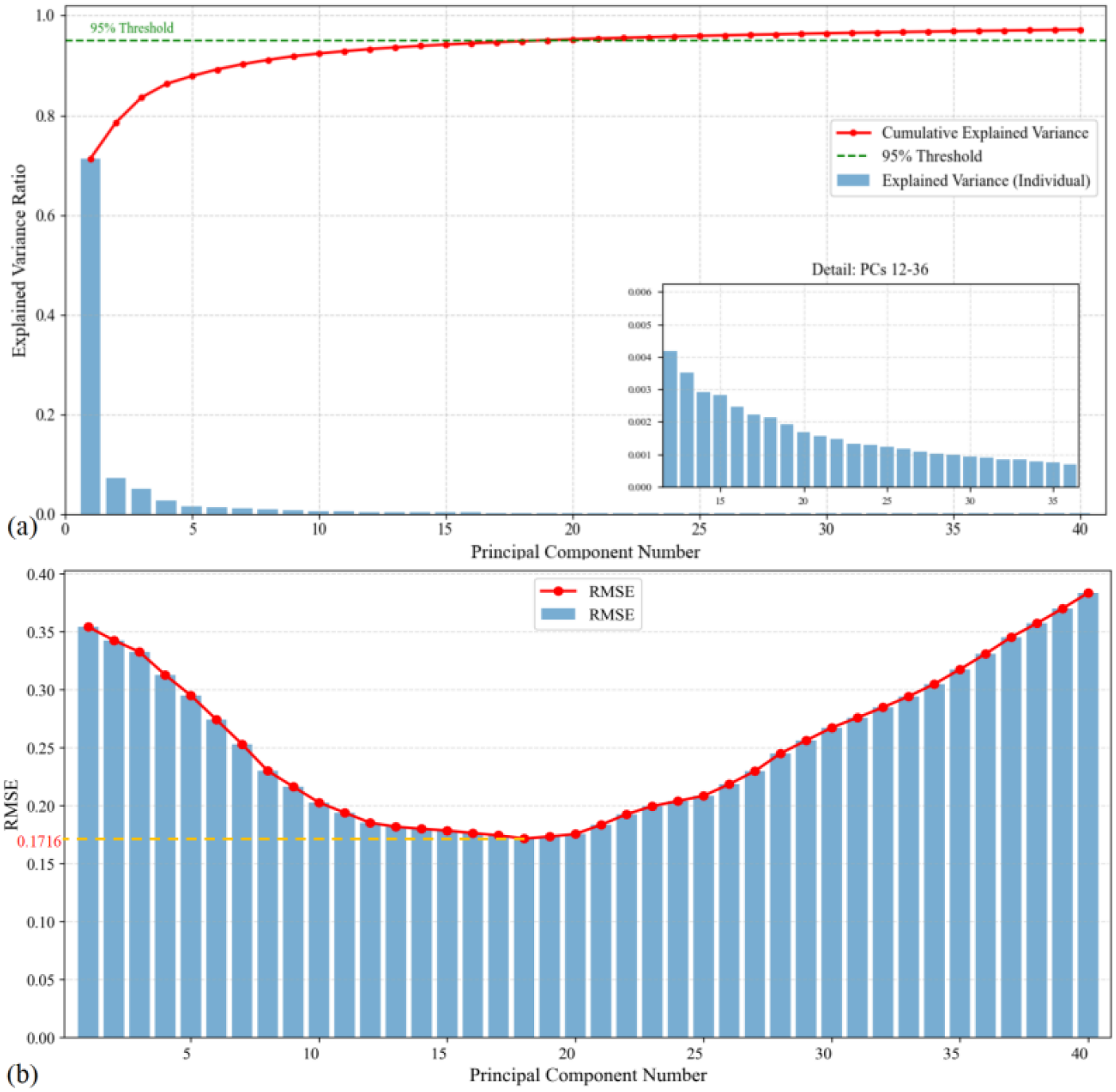
The relationship between the number of principal components, explained variance ratio, and prediction accuracy for 2022–2023. (a) Shows the variation of principal components with their corresponding explained variance ratios and cumulative explained variance ratios as the number of principal components increases. (b) Demonstrates the variation in 2022–2023 prediction accuracy with respect to the number of principal components.
As shown in Figures 5a, c, compared to the TOPAZ numerical model, Persistence and Climatology baseline models, the EOF-Trans consistently achieves the lowest root mean square error and the highest correlation coefficient in each year. This indicates that the predictions from EOF-Trans are closest to the actual observations and exhibit the best statistical correlation, fully demonstrating the superior performance in sea ice thickness prediction. As a classical numerical model, TOPAZ also demonstrates strong predictive capability, with its RMSE remaining stable between 0.20–0.25 m in most years and Corr ranging from 0.65 to 0.75. While both Persistence and Climatology provide basic forecasting skill, Climatology performs significantly better than Persistence. Figures 5b, d further illustrate the prediction errors and correlation performance of EOF-Trans under different leadtime in 2022–2023. Benefiting from the ability to capture long-term temporal dependencies in Transformer, EOF-Trans exhibits strong stability. Although TOPAZ performs well in the initial lead days, its correlation declines significantly due to error accumulation. The Persistence model, which assumes that the current ice thickness distribution resembles the previous time step, performs particularly well in the first two lead times. However, its predictive skill deteriorates rapidly when significant changes in sea ice thickness occur. In contrast, Climatology reflects the average trend of ice thickness distribution, resulting in relatively stable but less dynamic predictions. In summary, EOF-Trans delivers the best overall performance, followed by Climatology, with TOPAZ and Persistence ranking successively lower.
Figure 5
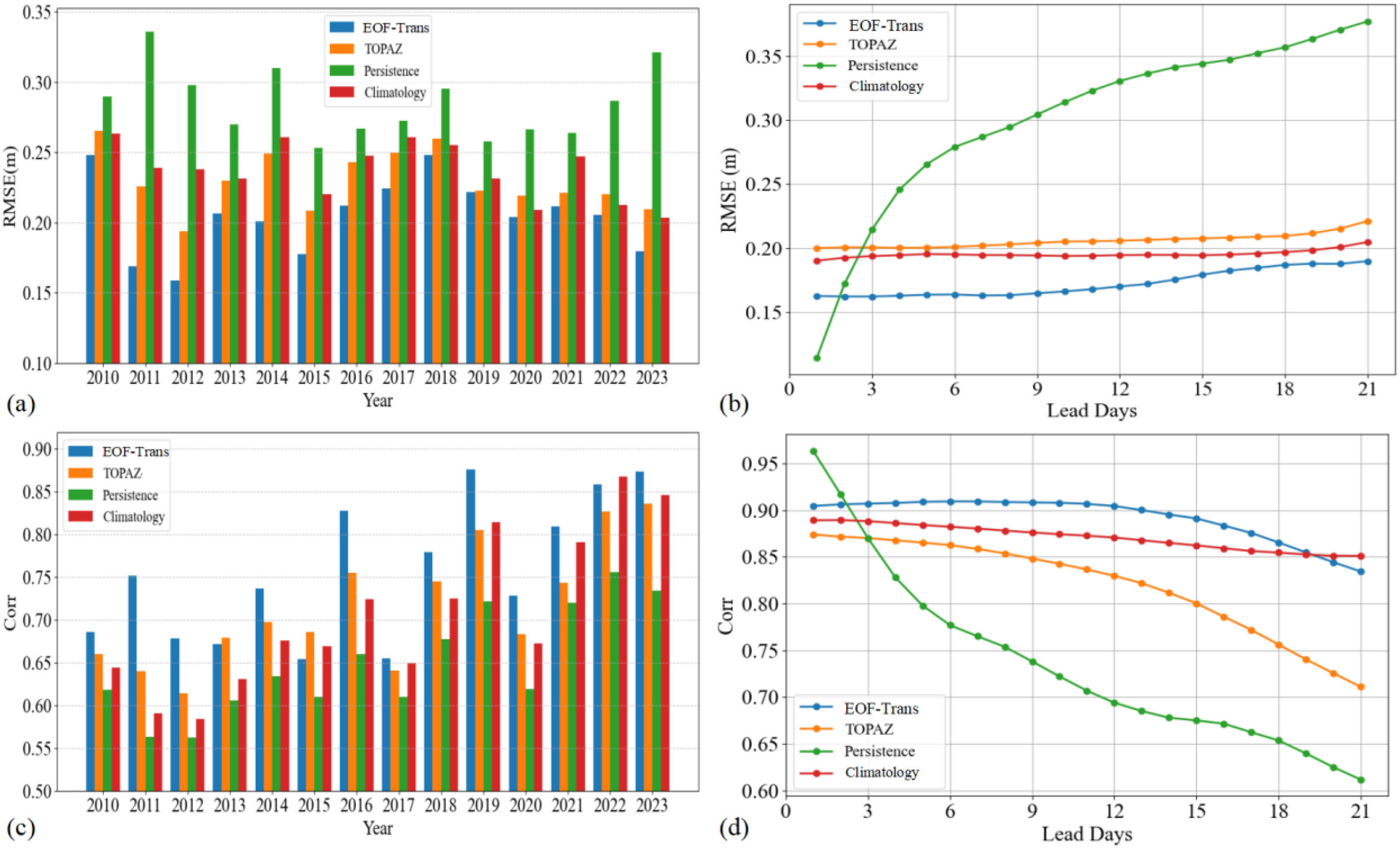
The performance comparison between EOF-Trans, numerical models, and baseline models. (a) and (c) show the performance comparison of RMSE and Corr between EOF-Trans and other models from 2010 to 2023, respectively. (b, d) illustrate the variations in RMSE and Corr for EOF-Trans and other models across different lead days during 2022–2023, respectively.
Figure 6 provides spatial and temporal examples comparing the differences between EOF-Trans prediction results and actual observations. The predicted results exhibit distinct spatial characteristics. As latitude increases, the SIT predicted by EOF-Trans gradually increases to 1.7 m. Thanks to the descriptive ability of EOFs for the overall characteristics of ice thickness, the results of EOF-Trans are relatively close to actual observations and can accurately predict the spatial distribution of SIT. From a temporal perspective, the prediction errors on the 7th, 14th, and 21st days gradually increase. Although the errors in EOF-Trans predictions increase with time, the spatial distribution of SIT it depicts remains consistent with actual observations. The description of the temporal context of SIT PCs by EOF-Trans ensures that its performance is still reliable even with larger lead days.
Figure 6
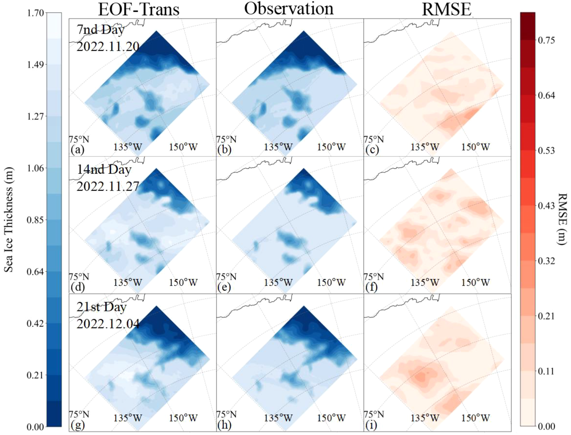
EOF-Trans results. From left to right are the predicted ice thickness, the observation value, and the RMSE between them. From top to bottom, they are the results for the 7th, 14th, and 21st days.
4.2 Comparison with the representative deep learning model
Although EOF-Trans outperforms both the baseline models and the numerical model, its relative advantages over other deep learning models require further comparison. Using cross-validation, this study evaluates the interannual variations and lead-time-dependent changes in the RMSE and correlation of EOF-Trans and four additional models, EOF-Markov, ConvLSTM, CNN, and U-Net, as shown in Figure 7. EOF-Trans consistently achieves the lowest RMSE and highest correlation across all years in Figures 7a, b, demonstrating the best overall prediction performance. Despite the increased prediction difficulty in 2010 and 2018, when all models exhibit RMSE values exceeding 0.25 due to strong Beaufort High anomalies (Kwok and Cunningham, 2015; Petty, 2018), EOF-Trans still maintains the lowest error among all models. U-Net generally performs better than ConvLSTM, suggesting that a deeper stacked convolutional structure provides advantages over the combination of convolution and recurrent memory mechanisms for sea ice thickness prediction. However, U-Net lacks explicit temporal context modeling, which may be an important reason why EOF-Trans outperforms U-Net in predictive skill. EOF-Markov and CNN also exhibit certain predictive capability but do not reach the performance level of EOF-Trans.
Figure 7
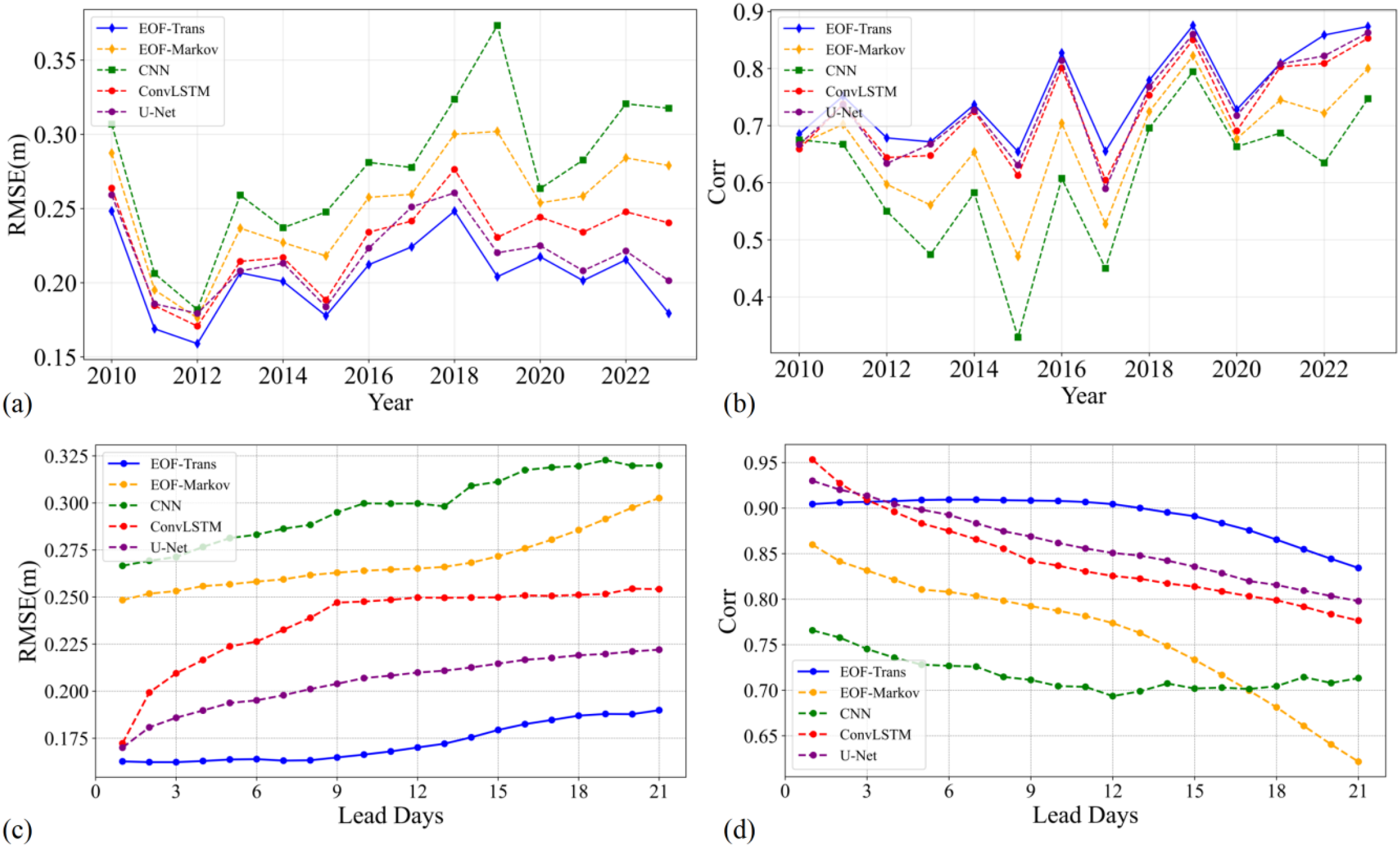
Performance comparison between EOF-Trans and other deep learning models at different years and different lead days. (a, b) RMSE and Corr comparison over years between 2010–2023. (c, d) RMSE and Corr comparison at different lead days in 2022–2023.
Further examination of the prediction performance of EOF-Trans and the deep learning models across different leadtime in Figures 7c, d reveals a high degree of consistency with the interannual comparison. The Transformer architecture enables effective associations between information at different time steps, allowing EOF-Trans to maintain relatively high accuracy even at extended leadtimes, thereby demonstrating strong stability in Figure 7c. U-Net, which adopts a direct prediction strategy, effectively mitigates error accumulation with increasing leadtime. In contrast, the memory mechanism in ConvLSTM leads to continuous error accumulation, negatively impacting its predictive performance. This explains why ConvLSTM exhibits higher correlations than EOF-Trans during the first three leadtimes, but subsequently experiences a rapid decline Figure 7d.
To evaluate the predictive reliability of the models, the results of three independent runs of EOF-Trans and the comparative models on the 2022–2023 test dataset are reported in Table 2. The EOF-Trans model attains a mean value of 0.8804 with a standard deviation of 0.0078, indicating a high degree of consistency across repeated experiments. The U-Net and ConvLSTM models exhibit similar levels of variability, however, U-Net demonstrates superior predictive performance relative to ConvLSTM. The performance of EOF-Markov and CNN is comparatively lower.
Table 2
| Model | EOF-Trans | EOF-Markov | U-Net | ConvLSTM | CNN |
|---|---|---|---|---|---|
| RMSE (m) | 0.1680 | 0.2986 | 0.2035 | 0.2416 | 0.3158 |
| Mean (std.) | (0.0076) | (0.0095) | (0.0085) | (0.0084) | (0.0087) |
| Corr | 0.8804 | 0.6310 | 0.8597 | 0.8283 | 0.6755 |
| Mean (std.) | (0.0078) | (0.0093) | (0.0084) | (0.0085) | (0.0096) |
Performance (mean and standard deviation, std.) comparison between EOF-Trans and other models at 2022–2023.
The bold values indicate the best performance.
Furthermore, the spatial distributions of prediction bias for EOF-Trans, ConvLSTM, and U-Net at different leadtime are shown in Figure 8. The prediction biases of all models are primarily concentrated in regions with strong sea ice variability, where they tend to underestimate thin ice and overestimate thick ice. This spatial pattern becomes more pronounced as the leadtime increases. However, EOF-Trans exhibits smaller bias magnitudes and more localized bias regions, indicating superior model stability. In contrast, ConvLSTM and U-Net fail to accurately capture the detailed evolution of sea ice, showing noticeable deviations as early as lead time 7, with the discrepancy further amplified at longer leadtimes. Although ConvLSTM demonstrates prediction skills comparable to EOF-Trans in certain local areas, its insufficient consideration of interregional dependencies leads to suboptimal reconstruction of the overall spatial distribution of ice thickness, indirectly highlighting the effectiveness of EOF-based global feature extraction. U-Net, being a fully convolutional architecture, relies entirely on convolutional operations for spatial feature extraction. While this enables relatively good spatial modeling capability, its limited receptive field results in notable prediction inconsistencies across different local regions, making its overall performance slightly inferior to that of EOF-Trans.
Figure 8
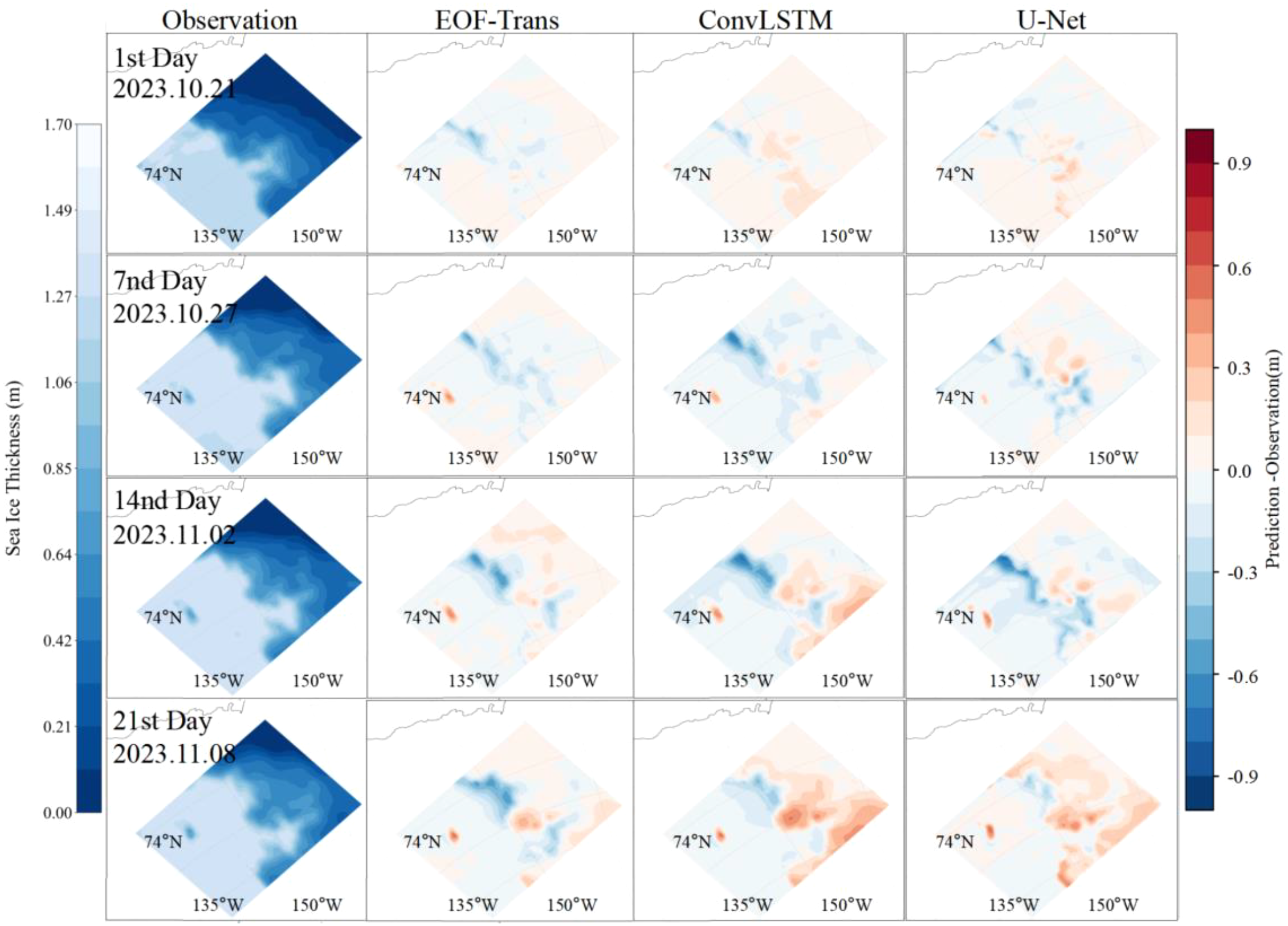
The spatial distributions of observation and prediction biases, namely prediction – observation, for EOF-Trans, ConvLSTM, and U-Net at leadtime of 1, 7, 14, and 21. The first column represents the observed values, and the second, third, and fourth columns represent EOF-Trans, ConvLSTM, and U-Net, respectively.
4.3 Explainability analysis of EOF-Trans
To further examine how EOF-Trans utilizes temporal information, this study conducts a visualization analysis of the multi-head attention weights in the Transformer decoder. Figure 9 presents the attention weight distributions of the three attention heads, based on statistics derived from the 2022–2023 test dataset. Overall, the multi-head attention mechanism enables EOF-Trans to attend to information across different temporal ranges, thereby forming a multi-level representation of short-term dependencies, intermediate lagged relationships, and longer-term temporal structures present in the spatiotemporal variability of SMOS-retrieved sea ice thickness.
Figure 9
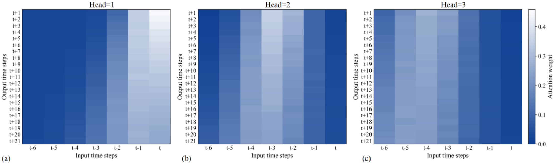
Attention weight distribution of EOF-Trans. (a–c) represent the attention weight distributions of the 1st, 2nd, and 3rd heads, respectively.
Among the three attention heads, Head 1 exhibits a pronounced emphasis on recent inputs, with future predictions assigning the highest weights to the most recent time steps (i.e., t, t-1, and t-2), while contributions from earlier time steps gradually decrease and remain relatively low Figure 9a. This pattern indicates that the model places greater statistical importance on short-term temporal continuity and autocorrelation in the SMOS-retrieved sea ice thickness data, suggesting that this head primarily captures rapid variations at short temporal scales. In contrast, Head 2 shows a more distributed attention pattern, with relatively higher weights assigned to inputs from t-2 to t-4 Figure 9b. This behavior reflects the model’s ability to incorporate lagged temporal dependencies spanning several days, representing accumulated influences embedded in the SMOS-retrieved sea ice thickness data without explicitly resolving specific physical drivers. Head 3 displays the most uniform attention distribution across time steps Figure 9c, indicating a tendency to aggregate information over the entire temporal window of the SMOS-derived sea ice thickness sequence. Such global attention supports the extraction of broader temporal tendencies in the input sequence and contributes to maintaining stable predictions at longer lead times.
4.4 Error and uncertainty analysis
To assess the reliability of the model predictions, this study compares the kernel density distributions of the predicted RMSE and the inherent retrieval uncertainty of the SMOS L3 sea ice thickness product over the 2022–2023 test period Figure 10. As shown in Figure 10a, the RMSE distribution exhibits a unimodal pattern, with the density peak corresponding to an RMSE of approximately 0.23 m. More than 90% of the samples fall within the range of 0.10–0.25 m, indicating that the model’s prediction errors are generally low and exhibit limited variability.
Figure 10
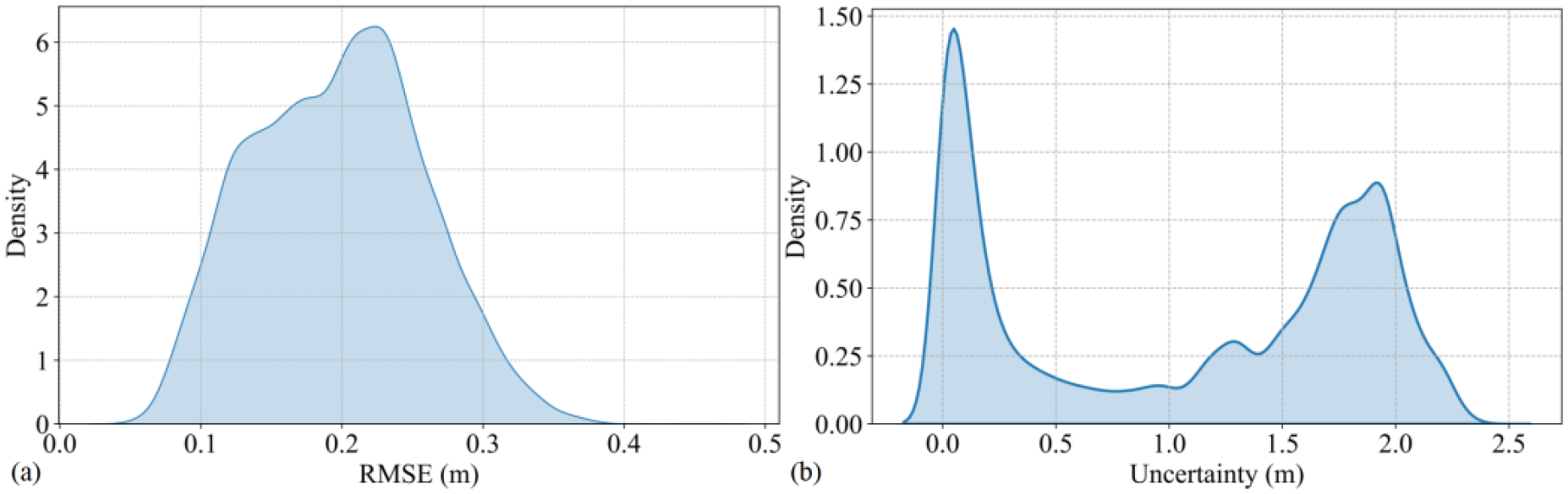
KDE kernel density distribution of RMSE and data uncertainty of SMOS L3 SIT in the test dataset during 2022–2023. (a) KDE density of RMSE from EOF-Trans in the test dataset. (b) KDE density of SMOS L3 SIT data uncertainty in the test dataset.
In contrast, the uncertainty distribution of the SMOS L3 product Figure 10b presents a distinct bimodal structure. The first density peak occurs within the 0.0–0.5 m range, representing regions with relatively low retrieval uncertainty, while the second peak, located between 1.5 and 2.0 m, corresponds to ice conditions where the retrieval uncertainty is substantially higher. The comparison reveals that the RMSE of EOF-Trans is lower than the primary uncertainty level of the SMOS L3 data, suggesting a potential tendency to fit observational noise or biases. Nevertheless, when considered together with the preceding analyses, these results indicate that EOF-Trans primarily learns and reproduces the spatiotemporal regularities embedded in the SMOS-retrieved sea ice thickness fields. It is worth noting that the proposed framework is trained on satellite-retrieved sea ice thickness fields, and its learned representations therefore reflect the dominant spatiotemporal patterns present in the SMOS product. The extent to which these patterns can be directly associated with the underlying physical processes of sea ice thickness evolution remains uncertain and warrants further investigation.
5 Conclusions
Under the influence of global warming, Arctic sea ice thickness has exhibited a pronounced and accelerating thinning trend, particularly during the early freezing season when thin ice dominates large areas of the Arctic Ocean. Accurate daily-scale prediction of sea ice thickness under these conditions provides valuable support for characterizing short-term sea ice variability. While existing studies have made progress in sea ice thickness prediction, limitations remain in effectively capturing the large-scale spatial structures and temporal contextual dependencies present in satellite-derived sea ice thickness fields. To address this challenge, this study proposes a spatiotemporal prediction framework, EOF-Trans, designed for forecasting daily variations of thin sea ice thickness with lead times of up to 21 days during the early freezing season. The framework integrates Empirical Orthogonal Function (EOF) decomposition with a Transformer architecture to achieve spatiotemporal prediction through decomposition, temporal forecasting, and reconstruction of the SMOS-retrieved sea ice thickness field.
Experimental results for the Beaufort Sea over the period 2010–2023 demonstrate that EOF-Trans achieves higher predictive skill than numerical model outputs and commonly used deep learning approaches such as U-Net and ConvLSTM. The model exhibits stable temporal performance and enhanced spatial representation capability, with spatial biases generally remaining below 0.5 m even at extended lead times. These results highlight the effectiveness of EOF-Trans in capturing dominant spatiotemporal regularities embedded in the SMOS-derived sea ice thickness product. Further analyses comparing model errors with data uncertainty indicate that, although EOF-Trans may partially reflect product-specific noise or bias, its predictions are primarily governed by coherent statistical patterns present in the input data. In addition, attention-weight analysis suggests that the Transformer component learns multiscale spatiotemporal dependencies, providing a phenomenological and data-driven basis for model interpretability.
Despite these advantages, several limitations of this study should be acknowledged. The predictive skill of EOF-Trans primarily reflects its ability to learn spatiotemporal regularities embedded in the SMOS L3-retrieved sea ice thickness fields, rather than explicitly resolving the underlying physical dynamics of sea ice evolution. As a result, product-specific characteristics, including retrieval uncertainty, noise, and potential systematic biases, may be partially inherited by the model predictions. At present, the proposed framework does not allow for a clear separation between regularities driven by the SMOS product and those arising from true physical processes, which constitutes an important limitation of this study. In addition, the applicability of the model to other regions, thicker ice regimes, or future periods remains constrained by the spatiotemporal coverage of the available training data. Future work will focus on integrating multi-source observational and reanalysis datasets to better disentangle product-driven features from physical mechanisms and to enhance the robustness and interpretability of the proposed framework.
Statements
Data availability statement
The original contributions presented in the study are included in the article/Supplementary Material. Further inquiries can be directed to the corresponding author.
Author contributions
LJ: Conceptualization, Methodology, Software, Writing – original draft. ZG: Conceptualization, Writing – review & editing, Software, Writing – original draft, Methodology. XS: Validation, Writing – review & editing. GM: Writing – review & editing, Validation. LP: Writing – review & editing, Formal analysis, Data curation. WD: Writing – review & editing, Formal analysis, Data curation. ZB: Writing – review & editing, Formal analysis, Data curation.
Funding
The author(s) declared that financial support was received for this work and/or its publication. This study was funded in part by the National Natural Science Foundation of China Grant 41876105, 41371436, in part by the Henan Province Natural Science Foundation 242300421043 to SX.
Conflict of interest
The author(s) declared that this work was conducted in the absence of any commercial or financial relationships that could be construed as a potential conflict of interest.
Generative AI statement
The author(s) declared that generative AI was not used in the creation of this manuscript.
Any alternative text (alt text) provided alongside figures in this article has been generated by Frontiers with the support of artificial intelligence and reasonable efforts have been made to ensure accuracy, including review by the authors wherever possible. If you identify any issues, please contact us.
Publisher’s note
All claims expressed in this article are solely those of the authors and do not necessarily represent those of their affiliated organizations, or those of the publisher, the editors and the reviewers. Any product that may be evaluated in this article, or claim that may be made by its manufacturer, is not guaranteed or endorsed by the publisher.
Supplementary material
The Supplementary Material for this article can be found online at: https://www.frontiersin.org/articles/10.3389/fmars.2026.1657592/full#supplementary-material
References
1
Andersson T. R. Hosking J. S. Pérez-Ortiz M. Paige B. Elliott A. Russell C. et al . (2021). Seasonal Arctic sea ice forecasting with probabilistic deep learning. Nat. Commun.12, 5124. doi: 10.1038/s41467-021-25257-4
2
Ashish V. Shazeer N. Parmar N. Uszkoreit J. Jones L. Gomez A. N. et al . (2023). Attention is All You Need. Available online at: http://arxiv.org/abs/1706.03762 (Accessed October 11, 2024).
3
Chi J. Bae J. Kwon Y.-J. (2021). Two-stream convolutional long- and short-term memory model using perceptual loss for sequence-to-sequence arctic sea ice prediction. Remote Sens.13, 3413. doi: 10.3390/rs13173413
4
Chi J. Kim H. (2017). Prediction of arctic sea ice concentration using a fully data driven deep neural network. Remote Sens.9, 1305. doi: 10.3390/rs9121305
5
Derry A. Krzywinski M. Altman N. (2023). Convolutional neural networks. Nat Methods. 20, 1269–1270. doi: 10.1038/s41592-023-01973-1
6
Deser C. Walsh J. E. Timlin M. S. (2000). Arctic sea ice variability in the context of recent atmospheric circulation trends. J. Climate13, 617–633. doi: 10.1175/1520-0442(2000)013<0617:ASIVIT>2.0.CO;2
7
Durand C. Finn T. S. Farchi A. Bocquet M. Boutin G. Ólason E. (2024). Data-driven surrogate modeling of high-resolution sea-ice thickness in the Arctic. Cryosphere18, 1791–1815. doi: 10.5194/tc-18-1791-2024
8
Feng J. Li J. Zhong W. Wu J. Li Z. Kong L. et al . (2023). Daily-scale prediction of arctic sea ice concentration based on recurrent neural network models. JMSE11, 2319. doi: 10.3390/jmse11122319
9
Guo Y. Yu Y. Lin P. Liu H. He B. Bao Q. et al . (2020). Simulation and improvements of oceanic circulation and sea ice by the coupled climate system model FGOALS-f3-L. Adv. Atmospheric Sci.37, 1133–1148. doi: 10.1007/s00376-020-0006-x
10
Gupta M. Caya A. Buehner M. (2021). Assimilation of SMOS sea ice thickness in the regional ice prediction system. Int. J. Remote Sens.42, 4583–4606. doi: 10.1080/01431161.2021.1897183
11
He J. Zhao Y. Yang D. Zhu K. Deng X. (2022). “ An Improved ConvLSTM Network for Arctic Sea Ice Concentration Prediction,” in OCEANS 2022, Hampton Roads ( IEEE, Hampton Roads, VA, USA), 1–5. doi: 10.1109/OCEANS47191.2022.9977029
12
Hochreiter S. Schmidhuber J. (1997). Long short-term memory. Neural Comput.9, 1735–1780. doi: 10.1162/neco.1997.9.8.1735
13
Huntington H. P. Daniel R. Hartsig A. Harun K. Heiman M. Meehan R. et al . (2015). Vessels, risks, and rules: Planning for safe shipping in Bering Strait. Mar. Policy51, 119–127. doi: 10.1016/j.marpol.2014.07.027
14
Junhwa C. Hyun-Cheol K. (2021). Retrieval of daily sea ice thickness from AMSR2 passive microwave data using ensemble convolutional neural networks. GIScience Remote Sens.58, 812–830. doi: 10.1080/15481603.2021.1943213
15
Kaleschke L. Tian-Kunze X. Maaß N. Beitsch A. Wernecke A. Miernecki M. et al . (2016). SMOS sea ice product: Operational application and validation in the Barents Sea marginal ice zone. Remote Sens. Environ.180, 264–273. doi: 10.1016/j.rse.2016.03.009
16
Kaleschke L. Tian-Kunze X. Maaß N. Mäkynen M. Drusch M. (2012). Sea ice thickness retrieval from SMOS brightness temperatures during the Arctic freeze-up period. \grl39, L05501. doi: 10.1029/2012GL050916
17
Kim Y. J. Kim H.-C. Han D. Lee S. Im J. (2020). Prediction of monthly Arctic sea ice concentrations using satellite and reanalysis data based on convolutional neural networks. Cryosphere. 14, 1083–1104. doi: 10.5194/tc-14-1083-2020
18
Kwok R. Cunningham G. F. (2015). Variability of Arctic sea ice thickness and volume from CryoSat-2. Philos. Trans. R. Soc. A: Mathematical Phys. Eng. Sci.373, 20140157. doi: 10.1098/rsta.2014.0157
19
Laxon S. W. Giles K. A. Ridout A. L. Wingham D. J. Willatt R. Cullen R. et al . CryoSat2 estimates of Arctic sea ice thickness and volume. Geophys. Res. Lett.40, 732–737. doi:10.1002/grl.50193
20
Lemieux J. Beaudoin C. Dupont F. Roy F. Smith G. C. Shlyaeva A. et al . (2016). The Regional Ice Prediction System (RIPS): verification of forecast sea ice concentration. Quart J. R. Meteoro Soc.142, 632–643. doi: 10.1002/qj.2526
21
Li W. Hsu C.-Y. Tedesco M. (2024). Advancing Arctic sea ice remote sensing with AI and deep learning: now and future. Remote Sens. 16, 3764. doi: 10.3390/rs16203764
22
Lindsay R. W. Zhang J. (2005). The thinning of arctic sea ice 1988-2003: have we passed a tipping pointJ. Climate18, 4879–4894. doi: 10.1175/JCLI3587.1
23
Liu J. Lei R. Song M. Xu S. Ji S. Su J. et al . (2021). Development and challenge of sea ice model adapting to rapid polar sea ice changes. Trans. Atmos Sci.44, 12–25.
24
Madsen K. S. Rasmussen T. A. S. Ribergaard M. H. Ringgaard I. M. (2016). High resolution sea-ice modelling and validation of the arctic with focus on south Greenland waters 2004-2013. Polarforschung;85, 101–105 . doi: 10.2312/POLFOR.2016.006
25
Mu L. Liang X. Yang Q. Liu J. Zheng F. (2019). Arctic Ice Ocean Prediction System: evaluating sea-ice forecasts during ’s first trans-Arctic Passage in summer 2017. J. Glaciol.65, 813–821. doi: 10.1017/jog.2019.55
26
Notz D. Bitz C. M. (2017). “ Sea ice in Earth system models,” in Sea Ice, 304–325. doi: 10.1002/9781118778371.ch12
27
Petty A. A. (2018). A possible link between winter arctic sea ice decline and a collapse of the beaufort high? Geophysical Res. Lett.45, 2879–2882. doi: 10.1002/2018GL077704
28
Petty A. A. Kurtz N. T. Kwok R. Markus T. Neumann T. A. (2020). Winter arctic sea ice thickness from ICESat-2 freeboards. J. Geophysical Research: Oceans125, e2019JC015764. doi: 10.1029/2019JC015764
29
Ponsoni L. Massonnet F. Fichefet T. Chevallier M. Docquier D. (2019). On the timescales and length scales of the Arctic sea ice thickness anomalies: a study based on 14 reanalyses. Cryosphere. 13, 521–543. doi: 10.5194/tc-13-521-2019
30
Reichstein M. Camps-Valls G. Stevens B. Jung M. Denzler J. Carvalhais N. et al . (2019). Deep learning and process understanding for data-driven Earth system science. Nature566, 195–204. doi: 10.1038/s41586-019-0912-1
31
Ricker R. Hendricks S. Helm V. Skourup H. Davidson M. (2014). Sensitivity of CryoSat-2 Arctic sea-ice freeboard and thickness on radar-waveform interpretation. Cryosphere8, 1607–1622. doi: 10.5194/tc-8-1607-2014
32
Ricker R. Hendricks S. Kaleschke L. Tian-Kunze X. King J. Haas C. (2017). A weekly Arctic sea-ice thickness data record from merged CryoSat-2 and SMOS satellite data. Cryosphere. 11, 1607–1623. doi: 10.5194/tc-11-1607-2017
33
Ricker R. Lavergne T. Hendricks S. Paul S. Down E. Killie M. A. et al . (2025). Drift-aware sea ice thickness maps from satellite remote sensing. Cryosphere19, 3785–3803. doi: 10.5194/tc-19-3785-2025
34
Sakov P. Counillon F. Bertino L. Lisæter K. A. Oke P. R. Korablev A. (2012). TOPAZ4: an ocean-sea ice data assimilation system for the North Atlantic and Arctic. Ocean Sci.8, 633–656. doi: 10.5194/os-8-633-2012
35
Shi X. Chen Z. Wang H. Yeung D-Y. Wong W. K. Woo W. C . (2015). Convolutional lstm network: a machine learning approach for precipitation nowcasting. MIT Press. doi: 10.1007/978-3-319-21233-3_6
36
Smith G. Roy F. Reszka M. Colan D. S. He Z. Belanger J.-M. et al . (2016). Sea ice forecast verification in the canadian global ice ocean prediction system. Meteorol. Soc. 142, 659–671. doi: 10.1002/qj.2555
37
Tilling R. L. Ridout A. Shepherd A. Wingham D. J. (2015). Increased Arctic sea ice volume after anomalously low melting in 2013. Nat. Geosci.8, 643–646. doi: 10.1038/ngeo2489
38
Timmermans M.-L. Toole J. M. (2023). The arctic ocean’s beaufort gyre. Annu. Rev. Mar. Sci.15, 223–248. doi: 10.1146/annurev-marine-032122-012034
39
Wang Y. Yuan X. Bi H. Ren Y. Liang Y. Li C. et al . (2023). Understanding arctic sea ice thickness predictability by a markov model. J. Climate36, 4879–4897. doi: 10.1175/JCLI-D-22-0525.1
40
Wayand N. E. Bitz C. M. Blanchard-Wrigglesworth E. (2019). A year-round subseasonal-to-seasonal sea ice prediction portal. Geophysical Res. Lett.46, 3298–3307. doi: 10.1029/2018GL081565
41
Wiebke A. Eriksson L. E. B. Ye Y. Heuzé C. (2020). First-year and multiyear sea ice incidence angle normalization of dual-polarized sentinel-1 SAR images in the beaufort sea. IEEE J. OF SELECTED TOPICS IN Appl. Earth OBSERVATIONS AND Remote Sens.13. doi: 10.1109/JSTARS.2020.2977506
42
Xi L. Fu Z. Chunhua L. Lin Z. Bingrui L . (2020). Evaluation of ArcIOPS sea ice forecasting products during the ninth CHINARE-Arctic in summer 2018. Advances in Polar Science. 31 (1), 14–25. doi: 10.13679/j.advps.2019.0019
43
Xie J. Counillon F. Bertino L. Tian-Kunze X. Kaleschke L. (2016). Benefits of assimilating thin sea ice thickness \hack\newlinefrom SMOS into the TOPAZ system. Cryosphere10, 2745–2761. doi: 10.5194/tc-10-2745-2016
44
Yuan X. Chen D. Li C. Wang L. Wang W. (2016). Arctic sea ice seasonal prediction by a linear markov model. J. Climate29, 8151–8173. doi: 10.1175/JCLI-D-15-0858.1
Summary
Keywords
arctic, deep learning, spatiotemporal prediction, thin sea ice thickness, transformer
Citation
Liu J, Zhang G, Xing S, Gao M, Li P, Wang D and Zheng B (2026) Daily-scale spatiotemporal prediction of thin sea ice thickness during the early freezing season based on EOF-Trans. Front. Mar. Sci. 13:1657592. doi: 10.3389/fmars.2026.1657592
Received
01 July 2025
Revised
24 January 2026
Accepted
28 January 2026
Published
16 February 2026
Volume
13 - 2026
Edited by
Francisco Machín, University of Las Palmas de Gran Canaria, Spain
Reviewed by
Miguel Angel Ahumada-Sempoal, University of the Sea, Mexico
Weibin Chen, University College London, United Kingdom
Updates
Copyright
© 2026 Liu, Zhang, Xing, Gao, Li, Wang and Zheng.
This is an open-access article distributed under the terms of the Creative Commons Attribution License (CC BY). The use, distribution or reproduction in other forums is permitted, provided the original author(s) and the copyright owner(s) are credited and that the original publication in this journal is cited, in accordance with accepted academic practice. No use, distribution or reproduction is permitted which does not comply with these terms.
*Correspondence: Shuai Xing, xing972403@163.com
Disclaimer
All claims expressed in this article are solely those of the authors and do not necessarily represent those of their affiliated organizations, or those of the publisher, the editors and the reviewers. Any product that may be evaluated in this article or claim that may be made by its manufacturer is not guaranteed or endorsed by the publisher.