Abstract
The effective monitoring of dynamic marine phenomena, such as phytoplankton blooms, across multiple spatial and temporal scales remains challenging. However, emerging closed-loop observation systems which integrate adaptive, multi-platform sensors with operational ocean models offer substantial potential to enhance accuracy and responsiveness. An operational closed-loop state estimation system was developed and tested in near real-time during a two-month field campaign in Frohavet, Norway. This closed-loop system integrated an Ensemble Kalman Filter with a coupled physical–chemical–biological ocean model across nested domains from the North Atlantic shelf to local coastal regions. Observations from the agile CubeSat HYPSO-1 nano-satellite and an uncrewed surface vehicle (USV, AutoNaut) were assimilated, dynamically informing the USV’s navigation and demonstrating the feasibility of adaptive, multi-tiered monitoring. Incorporating HYPSO-1 chlorophyll-a observations improved phytoplankton estimates at regional scales, while assimilating USV-based chlorophyll-a data further refined the predictions locally. The campaign highlighted operational challenges, including communication delays, software constraints, persistent cloud coverage, and solar storms. Post-campaign analyses identified and mitigated ecosystem model biases related to silicate dynamics and fixed carbon:nitrogen:chlorophyll-a conversion factors, further improving the model accuracy. Addressing these limitations through greater automation, tighter integration, and robust contingency planning is critical to scaling future closed-loop ocean monitoring systems.
1 Introduction
Monitoring the global ocean has become increasingly crucial as the physical, chemical, and biological processes are significantly impacted by human activities, such as overfishing, chemical and noise pollution, habitat loss, carbon dioxide (CO2) emissions, ocean acidification, and sea surface warming (Loeng and Drinkwater, 2007; Doney et al., 2012; Bates et al., 2014; Intergovernmental Panel on Climate Change (IPCC), 2022a, Intergovernmental Panel on Climate Change (IPCC), 2022b, Intergovernmental Panel on Climate Change (IPCC), 2023). To better understand and mitigate these effects, comprehensive monitoring is needed across the spatial and temporal scales at which these processes occur. Operational ocean monitoring systems often utilize a variety of observational platforms, such as satellites, buoys, uncrewed surface vehicles (USVs) and autonomous underwater vehicles (AUVs). Large-scale satellite systems provide extensive spatial coverage and capture broad environmental patterns, but typically have long revisit intervals and thus limited temporal resolution at a given location. In contrast, in situ sampling offers ground-truth point data with high temporal resolution, which is essential for validating remotely-sensed observations. Small satellites and uncrewed aerial vehicles (UAVs) can provide coverage at intermediate temporal and spatial scales, collecting high-resolution data in selected areas and times. Similarly, USVs and AUVs collect detailed information at the ocean’s surface and depths. The study presented here investigates how a coordinated small-satellite–USV system, coupled to an ocean model, can be used to realize a closed-loop observing framework during a coastal spring-bloom event.
Operational oceanography has progressed substantially in recent decades, with advances in biogeochemical sensing, expanded spatial and temporal coverage (including below 2000 m), finer-resolution numerical models, tighter coupling between physical, biogeochemical and sea-ice systems, and increasing use of ensemble-based approaches for uncertainty quantification and forecast reliability (Legler et al., 2015; Tonani et al., 2015; Schiller et al., 2015, Schiller et al., 2018). Despite these developments, many systems still function in an open-loop configuration where observation patterns are predetermined, and observations do not directly influence the real-time deployment or trajectories of other observational assets. In contrast, closed-loop systems continuously assimilate observations into ocean models to predict future states, which, in turn, inform and adapt the deployment of assets such as USVs and AUVs. This feedback mechanism enables adaptive tasking and improves the spatio-temporal efficiency and accuracy of ocean monitoring.
While this concept is gaining traction, fully integrated closed-loop systems are not yet standard in operational oceanography, as many observational platforms are passive buoys or satellites. For instance, the U.S. Integrated Ocean Observing System (IOOS) and the European Copernicus Marine Service provide comprehensive ocean monitoring by integrating diverse data sources and using data assimilation to improve model accuracy. However, their largely non-maneuverable sensors continue to sample along predetermined tracks, without real-time redirection informed by those forecasts. Intelligent, feedback-capable autonomous platforms are now extending regional observing capacity and enabling real-time adaptive observing strategies, particularly through gliders and other mobile assets. Nonetheless, recent work emphasizes that fully event-based, closed-loop observing architectures remain rare in routine practice and will require further technological and systems-integration advances before they can be widely adopted (Schiller et al., 2018; Lermusiaux, 2007; Davidson et al., 2019).
At the same time, improved ocean reanalyses depend on stronger feedback loops between data-assimilation centers and adaptive observing networks. Although reanalyses themselves are produced retrospectively, they can reveal systematic model and observation gaps that inform the design of future observing strategies. In an operational context, adaptive observing systems guided by model uncertainty can focus sampling on regions with sparse data or high variability, thereby increasing the impact of observations and improving both real-time analyses and subsequent reanalyses. Penny et al. (2019) note that while many sensors have adaptive sampling capabilities, there is untapped potential for state feedback between operational ocean data assimilation systems and the guidance of observing systems in near real-time. Nevertheless, multi-vehicle operations are still constrained by proprietary control interfaces and vehicle-specific data formats, which impede automated near-real-time ingestion and coordinated deployment of heterogeneous platforms. Harris et al. (2020) address part of this challenge by deploying the Oceanids C2 micro-service architecture, which converts generic waypoints into platform-specific commands and standardises data streams. deYoung et al. (2019) articulates a vision for an All-Atlantic Ocean Observing System by 2030, emphasizing multi-disciplinary, multi-platform basin-wide observational capability. Thus, despite recent gains, full real-time integration and adaptability remain open challenges.
Complementing these system-level efforts, previous work has extensively explored the integration of various observational platforms with open-loop ocean models for optimal path planning. In such systems, information flow is typically unidirectional: either the ocean model informs the observational asset, or the asset corrects the ocean model or other tools to unify heterogeneous ocean observations. For instance, Fossum et al. (2019) embedded an adaptive sampling technique on an AUV using a Gaussian process (GP) to map and track subsurface Chl-a maxima; and Berget et al. (2018), Berget et al., 2022, Berget et al., 2023) demonstrated adaptive tracking of suspended material plumes using an onboard stochastic spatio-temporal proxy model initialised with data from the same complex model used in this paper. Ford et al. (2022) further present a closed-loop experiment with one glider, guided by a stochastic predictor and assimilated into a pseudo-operational setup.
The primary challenge in operational oceanography is to develop systems that can integrate diverse observational data in real time and adapt dynamically to changing ocean conditions. This study demonstrates the first proof-of-concept closed-loop approach using a multi-tiered observing system that combines complementary platforms operating across various spatial and temporal scales in a two-month-long field campaign. The system targets chlorophyll-a (Chl-a) as a proxy for phytoplankton biomass during the Norwegian spring bloom. In sub-polar seas, these blooms evolve on synoptic (days-to-weeks) timescales under the combined influence of advection, light, nutrient supply, temperature and zooplankton grazing (Sarmiento and Gruber, 2006; Behrenfeld and Boss, 2014; Fragoso et al., 2024). Their rapid and irregular development makes them an ideal test case for a closed-loop architecture in which adaptive assets are repeatedly re-tasked on the basis of near-real-time model forecasts. Departing from traditional methods that rely on passive observational platforms, the system architecture combines complementary space- and sea-based platforms to achieve coherent sampling across nested spatial and temporal scales, and integrates a complex ocean model with real-time feedback from these dynamic agents. Data streams are merged through an Ensemble Kalman Filter (EnKF) (Evensen, 2003) coupled to a 3D hydrodynamic–ecological model, and the resulting high-precision forecasts are used as state feedback in path planning for the adaptive platforms. This closed-loop architecture significantly enhances the responsiveness and precision of ocean monitoring, and illustrates how dynamic observational platforms can adapt to evolving ocean conditions, improving the accuracy and efficiency of ocean observations while pointing towards future operational implementations. Although the present experiment focuses on one small satellite and a USV, the full potential of the observational system includes the utilisation of large-scale satellites, small satellites, UAVs, USVs and AUVs, each equipped with heterogeneous sensors to collect detailed physical and biological data.
Frohavet, a sea area sheltered by the Froan archipelago along the middle of the Norwegian coast (Figure 1b) was chosen as the experimental location. This region is characterized by shallow bathymetry and a highly productive basin (Fragoso et al., 2024), which supports abundant fishing activities and a burgeoning aquaculture industry. During the spring months, Frohavet typically experiences one or more significant algal blooms, which are highly dynamic both spatially and temporally. Comprehensive monitoring is required to fully capture the growth dynamics of these blooms, making this region an excellent testing ground for the closed-loop approach. Previous field campaigns have been conducted in both Frohavet (April-May 2022 and 2023) (Williamson et al., 2023), and Kongsfjorden (May 2022) in Svalbard, with some of the tested sensors showing adaptive sampling capabilities (Mo-Bjørkelund et al., 2024), albeit with simplified onboard models and not integrated with other observational platforms. In the present experiment, the observation system consists of two platforms: HYPSO-1, a small, agile 6U satellite equipped with a hyperspectral imager providing Chl-a estimates (Bakken et al., 2023), and the AutoNaut, a long-endurance wave-propelled USV equipped with a wide range of scientific sensors for sampling biological and physical properties of the surface waters (Dallolio et al., 2019). The observational platforms are described in detail in Sec. 2.2.1 and Sec. 2.2.2, and their measurements are assimilated into the ocean model using the EnKF framework demonstrated in Halvorsen et al. (2022).
Figure 1
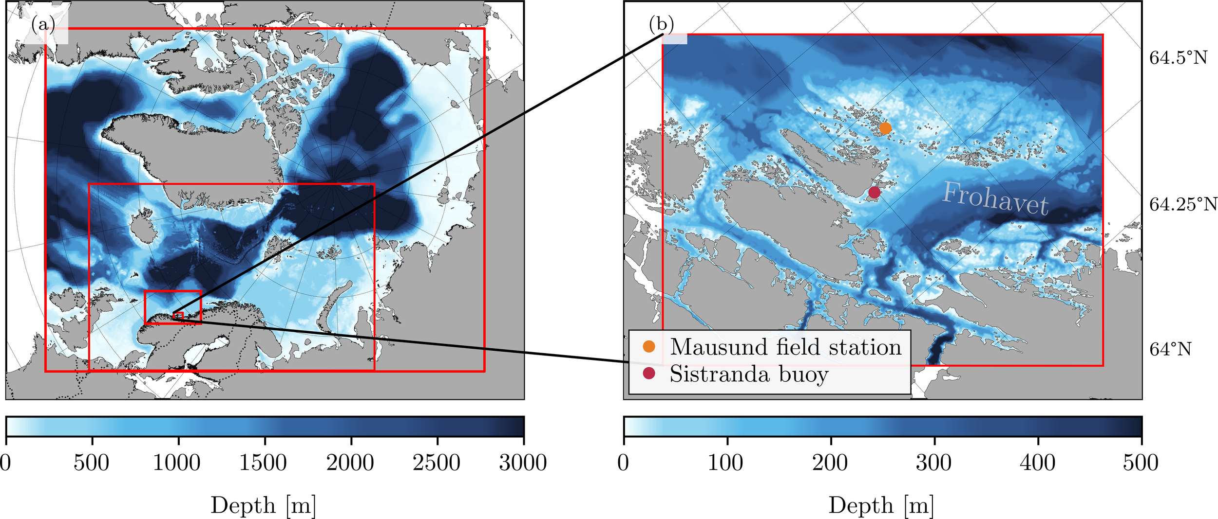
Overlaid bathymetry of (a) the North Atlantic–Arctic region with computational model domains GIN, NOR4KM, MIDNOR, and FROSHELF marked in red, and (b) a closer view of FROSHELF, marked in red, covering the Frohavet field campaign area, with marked locations for the Mausund field station and a research buoy at Sistranda.
2 Method
In this chapter, we introduce the required background and theory for understanding the campaign and methods. This includes a presentation of utilized models, data products and sensors.
2.1 Ocean model
The model used in this study is the coupled physical-chemical-biological ocean model SINMOD (Slagstad and McClimans, 2005; Wassmann et al., 2006), developed and maintained by SINTEF Ocean in Trondheim, Norway. With nearly 40 years of continuous refinement, SINMOD is designed to be a flexible research tool that allows efficient integration of new modelling strategies and configurations. SINMOD operates in a nested setup, where computational domains covering larger spatial scales are run at lower spatial and temporal resolutions, providing boundary conditions for smaller, higher-resolution domains. This approach follows the flow relaxation scheme of Martinsen and Engedahl (1987). The streamlined design of SINMOD, combined with its adaptability, enables the rapid testing of novel configurations and data assimilation methods, as applied in this study.
2.1.1 Model domains
The two principal coastal model domains used in this study have a horizontal resolution of 800 m, named MIDNOR, and 160 m, named FROSHELF. Two regional model domains of 20 km, referred to as GIN and 4 km, referred to as NOR4KM, are run simultaneously as support simulations for the production of boundary conditions for the two coastal model domains. The same model domain names are used to refer to the freerun simulations conducted in this study. To differentiate between simulations with and without data assimilation, an “a” prefix, for assimilation, is added to the domain names: aGIN, aNOR4KM, aMIDNOR and aFROSHELF. The computational domains are visualized in Figure 1.
The GIN model domain encompasses a large regional area capturing inflow from the North Atlantic, Nordic Seas, and Arctic Ocean, while also representing ice dynamics around Greenland, Baffin Bay, and the Arctic. The boundaries in this experiment are climatological data from World Ocean Circulation Experiment (WOCE) (Woods, 1985), and fixed fluxes. The vertical structure of the model comprises 25 z-layers, as detailed in Table 1.
Table 1
| Domain | Cumulative vertical discretization, [m] |
|---|---|
| GIN | 0, 10, 15, 20, 25, 30, 35, 40, 50, 75, 100, 150, 200, 250, 300, 400, 500, 700, 1000, 1500, 2000, 2500, 3000, 3500, 4000, 4500 |
| NOR4KM | 0, 10, 15, 20, 25, 30, 35, 40, 50, 75, 100, 150, 200, 250, 300, 350, 400, 450, 500, 550, 600, 650, 700, 750, 800, 850, 900, 1000, 1500, 2000, 2500, 3000, 3500, 4000, 4500 |
| MIDNOR | 0, 3, 6, 10, 15, 20, 25, 30, 35, 40, 50, 75, 100, 125, 150, 175, 200, 225, 250, 275, 300, 325, 350, 375, 400, 425, 450, 475, 500, 525, 550, 575, 600, 625, 650, 675, 725, 775, 825, 875, 925, 1025, 1150, 1275, 1400, 1525, 1775, 2025, 2275, 2525, 2775, 3025 |
| FROSHELF | 0, 3, 3.5, 4.0, 5.0, 6.0, 7.0, 8.0, 10.0, 12.0, 15.0, 20.0, 25.0, 30.0, 35.0, 40.0, 50.0, 75.0, 100.0, 150.0, 200.0, 250.0, 300.0, 350.0, 400.0, 450.0, 500.0, 550.0, 600.0, 650.0, 700.0, 750.0, 800.0, 850.0, 900.0, 1000.0, 1500.0, 2000.0, 2500.0, 3000.0 |
Cumulative vertical z-layer discretization for the four model domains.
The NOR4KM model domain covers a regional area with a horizontal resolution of 4 km, providing enhanced resolution of ocean features along the Norwegian coast, the surrounding Nordic seas, and parts of the Arctic. Boundary conditions for this domain are sourced from the GIN model domain. The model configuration includes 34 vertical layers listed in Table 1.
The MIDNOR domain features an 800-meter horizontal resolution and refined vertical discretization, enabling a detailed representation of complex coastal dynamics such as eddies, topographic upwelling, and fjord-shelf exchanges. These processes are challenging to resolve in coarser models with resolutions of 20 km or 4 km. This high-resolution domain is particularly critical for accurately simulating the Norwegian Coastal Current (NCC) and intricate coastal interactions. The model includes 50 vertical layers, described in Table 1.
The FROSHELF domain represents a high-resolution area encompassing the entrance to the Trondheim fjord, northeastern Smøla, Hitra, Frøya, and the Frohavet region. This configuration resolves key features of the archipelago and coastal processes with 39 vertical layers, outlined in Table 1.
2.1.2 Model forcing
Two different sources of atmospheric data are used. For the large-scale GIN and NOR4KM models, NOAA’s Global Forecast System (GFS)1 was used, which provides global data of 0.25-degree resolution with a 1-hour time resolution at a forecast horizon of 120 hours, and longer forecasts at a 3-hour time resolution. Initial conditions for GFS are provided by the Global Data Assimilation System (GDAS), which runs a 4D hybrid ensemble-variational data assimilation scheme. For the high-resolution MIDNOR and FROSHELF models, the Norwegian Meteorological Institute’s MetCoOp Ensemble Prediction System (MEPS)2 is used, which provides forecasts based on 30 ensemble members run every six hours with lead times out to 61 hours and a spatial grid spacing of 2.5 km. In both cases, data is downloaded in NetCDF format and linearly interpolated into each SINMOD domain’s grid. Atmospheric data is loaded by SINMOD every hour in model time, and linearly interpolated in time to fit the temporal resolution of the simulations.
For freshwater run-off, the model incorporates river discharges and diffuse land runoff as freshwater fluxes from the Hydrologiska Byråns Vattenbalansavdelning (HBV), Sweden, model (Beldring et al., 2003), provided by the Norwegian Water Resources and Energy Directorate (NVE).
2.1.3 Physical model
The ocean model’s hydrodynamic component is based on the hydrostatic primitive Navier-Stokes equations, which are discretized horizontally on an Arakawa C-grid with a polar stereographic projection and a z-coordinate system in the vertical. Each depth level has a fixed thickness, except at the surface and bottom layers, outlined in Tab. 1. A comprehensive description is provided in Slagstad and McClimans (2005).
2.1.4 Biology model
The ecosystem component of the ocean model, explained in detail by Wassmann et al. (2006), includes thirteen state variables: nitrate, ammonium, silicate, diatoms, flagellates, bacteria, heterotrophic nanoflagellates, microzooplankton, fast-sinking detritus, slow-sinking detritus, dissolved organic carbon, and two mesozooplankton species, Atlantic Calanus finmarchicus and Arctic Calanus glacialis. The primary unit of measurement is mmol N m−3. Conversion to carbon is done using the Redfield ratio, as described by Redfield et al. (1963).
Phytoplankton growth is influenced by available nutrients, sunlight and temperature conditions, all of which vary seasonally, latitudinally, and by the time of day. Planktonic organisms have limited control over their fine-scale distribution in the water column, relying primarily on ocean currents for horizontal and vertical transport. The transport equations, including all source and sink terms, are detailed in the appendix of Wassmann et al. (2006) and are solved numerically using a total variation diminishing (TVD) method.
Our work focuses on estimating Chl-a concentrations associated with the distribution of diatom and flagellate phytoplankton communities. The Chl-a concentration is calculated using the following relation from Equation 1:
where is the atomic ratio of carbon and nitrogen in marine phytoplankton, slightly enriched in carbon compared to the canonical Redfield ratio of (Redfield et al., 1963; Frigstad et al., 2014). MC = 12.01 g/mol is the molar mass of carbon. Fixed carbon-to-Chl-a ratios for diatoms and flagellates ( and ) were used, which are known to vary with environmental conditions such as light availability, temperature, and nutrient concentrations (Druon et al., 2010; Jakobsen and Markager, 2016; Yu et al., 2020; Smyth et al., 2023). A post-campaign sensitivity analysis was conducted to evaluate how variations in these conversion factors influence Chl-a estimates. Empirical values from the literature (MacIntyre et al., 2002; Sarthou et al., 2005; Lacour et al., 2017) informed the selection of a plausible range for CD (0.02–0.035) and CF (0.01–0.013).
2.2 The Frohavet monitoring campaign
The spring 2024 Frohavet ocean monitoring campaign started on the 2nd of April and concluded on the 21st of May. Bi-weekly meetings were held during the campaign to review data from the different sources in the closed-loop observation system, explained in detail in, 2.2.1 and 2.2.2. Observations were assimilated into the operational SINMOD model using an EnKF (Sections 2.4 and 2.3). The entire operational closed-loop ocean observation system is displayed in Figure 2. Additional data sources were monitored when available, irrespective of whether they were integrated into the closed-loop system. These sources included Chl-a estimates from ESA’s Sentinel-3A and 3B satellites (NASA Goddard Space Flight Center, 2024), NASA’s MODIS (NASA Ocean Biology Processing Group, 2025a) and VIIRS instruments (NASA Ocean Biology Processing Group, 2025b), and a Chl-a sensor installed at 3m depth on a kelp farm buoy about 2 km east of Frøya island (63°44.62’N 8°52.76’E) in the southern Frohavet region, shown in Figure 1b.
Figure 2
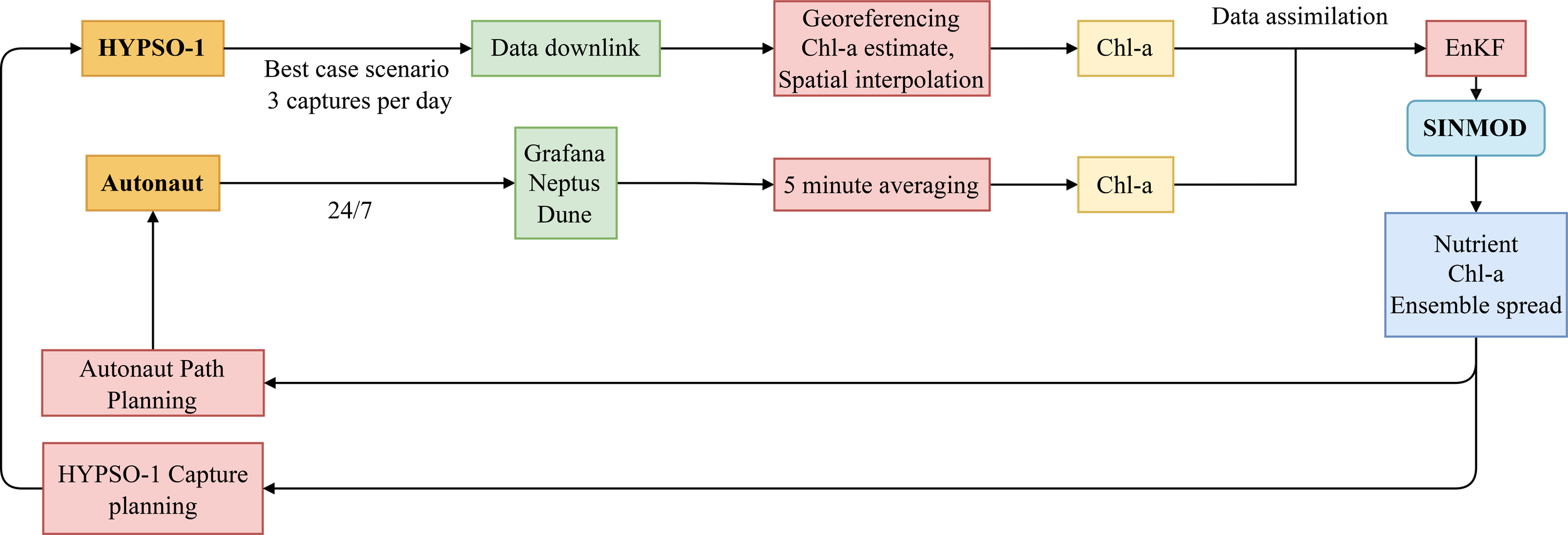
Schematic of the information flow from various observational sources and datasets into the operational model framework. The feedback loop includes the AutoNaut path planning, which was demonstrated in this experiment, and the HYPSO-1 capture planning.
2.2.1 The HYPSO-1 satellite
The HYPerspectral Small satellite for ocean Observation (HYPSO)-1 is a 6U CubeSat3, designed and operated by the Norwegian University of Science and Technology (NTNU). It carries a Hyperspectral Imaging (HSI) payload, sampling 120 spectral bands in the visible range (400–800 nm) (Grøtte et al., 2022; Bakken et al., 2023). These fine-band observations enable applications such as Chl-a estimation.
Launched in January 2022 into a Sun-synchronous 540 km Low Earth Orbit (LEO), HYPSO-1 has completed over 2000 hyperspectral observations. The satellite can be defined as agile due to its flexibility in pointing and target acquisition upon request (Langer et al., 2024), including multitarget tracking, wide swath imaging mode, and dynamic pointing captures, which could track complex, irregular coastlines (Langer et al., 2024).
The satellite captures 3–5 images daily, with a nominal nadir-view coverage of 300 km along-track by 70 km across-track, varying based on off-nadir angles. The satellite ground sampling distance is around 60 meters in the across-track direction and 320 meters in the along-track direction when imaging with nadir-pointing mode and sampling at a frame rate of 22 frames/s (Langer et al., 2024). Its orbit passes Norway north-to-south around 11:00 CET, providing 1–2 imaging opportunities daily over Frohavet. HYPSO-1 provides responsive targeting with higher tasking flexibility than systems with fixed imaging patterns and lower revisit frequency (Langer et al., 2024).
Priority imaging locations extended from Bergen to Rørvik, covering the MIDNOR computational domain (Figure 1a). HYPSO-1 captures underwent ground-based processing, including calibration, georeferencing, land and cloud masking, and Chl-a estimation. Radiometric calibration and destriping were performed using the HYPSO Python package4.
Georeferencing used an indirect approach that did not rely on onboard attitude or position telemetry. At least eight ground control points were manually selected in QGIS (QGIS Development Team, 2024), matching spatial features in RGB composites to known locations from Google Maps and OpenStreetMap. A second-order polynomial transform was fit using scikit-image, generating latitude and longitude matrices. Position uncertainty was limited by the HYPSO-1 RGB resolution (100–300 m, depending on imaging angle).
Chl-a estimates were derived using a 549 nm/663 nm band-ratio technique, leveraging chlorophyll absorption and reflectance properties (Henriksen, 2019, Henriksen, 2023). Since HYPSO-1 lacks exact 549 nm and 663 nm bands, the nearest available spectral bands (550 nm and 662 nm) were used after spectral calibration. The band-ratio method was applied only to unmasked regions, yielding relative Chl-a estimates.
Unprocessed HYPSO-1 captures (and future mission data) are available at https://www.ntnu.edu/web/smallsat/data-software, with specific datasets accessible upon request.
2.2.2 Uncrewed surface vehicle - AutoNaut
The AutoNaut is a commercially available 5 m-long USV with typical speeds up to 3 knots (Johnston and Poole, 2017) developed by AutoNaut Ltd, UK. It uses wave and solar power for propulsion, with an auxiliary thruster for calm conditions. Its passive propulsion enables extended operations, making it ideal for monitoring medium-to-large spatio-temporal phenomena (Dallolio et al., 2021).
Equipped with scientific environmental sensors, the AutoNaut measures key surface oceanographic variables, including Chl-a estimated from in-situ fluorescence measured by the WET Labs EcoPuck Triplet-W sensor5, and sea surface temperature (SST) and salinity (SSS) obtained from conductivity measurements using the SBE 49 FastCAT CTD6. The USV is controlled via the LSTS toolchain (Pinto et al., 2012), comprising Neptus for mission control (Dias et al., 2005), Dune for onboard processing, and IMC for communication (Martins et al., 2009). Real-time sensor data were visualized through a web interface7,8. The AutoNaut was deployed on the 6th of May 2024, and observations were gathered until the 16th of May 2024.
Chl-a fluorescence measurements were influenced by non-photochemical quenching (NPQ), a process whereby excess absorbed light energy is dissipated as heat, reducing fluorescence signals (Brunet et al., 2011; Welschmeyer, 2013; Travers-Smith et al., 2021). While algorithms to correct for NPQ effects exist, they require concurrent light measurements, which were not available during this campaign. The uncorrected observations were averaged into 5-minute intervals for assimilation to reduce high-frequency variability and instrument noise. Sensor-calibrated Chl-a concentrations were monitored for diurnal variations, confirming only weak NPQ effects during the campaign.
In a separate post-campaign analysis, the magnitude of NPQ effects was quantified using an approach similar to Fragoso et al. (2024). The observations were resampled to 1-second resolution, and local solar time was used as a proxy for light level to map non-quenched night-time fluorescence to daytime conditions and derive NPQ-corrected Chl-a concentrations, which are shown in Sec. 3.2.
2.2.3 Subsystem adaptive sampling
Although autonomous platforms can operate in closed loop, the situational awareness of a single vehicle is constrained by the footprint of its own sensors. Prior studies (Berget et al., 2018; Fossum et al., 2019; Berget et al., 2022, Berget et al., 2023) show that onboard Gaussian process estimators with simplified advection kernels allow a platform to fuse local measurements and to predict short term transport of key tracers. Operating several vehicles in tandem reduces regional uncertainty further, yet the combined picture is often obtained through lightweight probabilistic fusion rather than through a fully dynamic assimilation framework.
This work adopts a network perspective on adaptive observing. The proposed architecture is an adaptive observing system in which satellites, USVs, and AUVs stream observations into a conventional three dimensional ocean model. The model returns short range forecasts with uncertainty that serve as priors for the next sensing actions. These priors guide satellite target selection and waypoint planning for surface and underwater assets. By iterating this loop, the multi-agent network closes sampling gaps across scales and converges toward a self-consistent coastal state estimate.
During the 2024 Frohavet campaign a minimal configuration demonstrated the end-to-end loop from data ingestion through model update to adaptive retasking using one CubeSat and one wave-propelled USV.
2.2.3.1 HYPSO-1 target capture planning
Cloud cover frequently masked coastal targets, which is expected for this region in spring. A pre-declared fallback was therefore applied. When Frohavet was overcast at overpass time, HYPSO-1 prioritized clearer-sky targets south of the domain in the Bergen to Ålesund region so that mapped phytoplankton structures could advect northward with the NCC and enter the modeling domain within the forecast horizon. When Frohavet was predicted clear, it remained first priority. Persistent cloudiness during several overpasses precluded testing of more complex onboard retasking.
2.2.3.2 AutoNaut path planning
The AutoNaut can follow either a fixed survey pattern or a data-optimised route. In the past NTNU observational campaigns, a repetitive path was used to cover the whole area of interest (Oudijk et al., 2022; Williamson et al., 2023), providing broad coverage but no closed-loop adaptation. The latter would require the adoption of optimized path planning to analyze which locations are most interesting and valuable to observe. Closed-loop path planning was used to generate waypoint lists for the AutoNaut during the spring 2024 campaign. Waypoints were selected by solving an optimization problem that used aFROSHELF forecasts with assimilation of chl-a observations from HYPSO-1 and the USV. The optimization considers factors such as the uncertainty in forecasted Chl-a, the forecasted Chl-a daily increase, the USV’s current position, a worst-case speed of 0.2 m/s, and forecasted available nitrate in surface water to assess which points have higher relative priority of observation. The terms are normalised, weighted (ki) and summed into the dimensionless score of Equation 2
The four drivers for the score are:
-
Chl-a daily increase from the aFROSHELF simulation
-
Chl-a uncertainty from the aFROSHELF ensemble spread
-
Nitrate concentration at the surface layer from the aFROSHELF simulation
-
Distance of waypoint from (initial) AutoNaut position
Chl-a growth flags incipient blooms, ensemble spread represent areas of model uncertainty, nitrate reflects growth potential and distance penalises far-field targets given the wave-propelled speed constraint.
Each fi linearly rescales its parameter to [0, 1] from worst to best. Table 2 lists the normalization formulae and weight sets for early (Case 1) and late (Case 2) mission phases. In the first part of the campaign, nitrates concentration was not considered, as shown for case 1, while it was introduced towards the end of the mission for case 2. The adaptive search was restricted to a designated low-traffic box (63.8333°N - 63.9167°N, 9.0000°E - 9.1667°E). Scores are computed on the FROSHELF grid, where the score field, J, identifies locations of high observational value. The top 11 candidate waypoints are selected iteratively by choosing the grid cell with the highest score, then successively selecting the next highest-scoring cells that are at least 800 m away from any previously chosen point. A travelling-salesman solver then orders these waypoints to minimise the total path length from the USV’s current position (Applegate et al., 2006). The list of coordinates is then sent to the AutoNaut operator, who proceeds with tasking the agent. If the waypoint list was completed before the next planning update, temporary coordinates were sampled uniformly within the predefined operational box until replanning.
Table 2
| Parameter | Function | Case1 | Case 2 |
|---|---|---|---|
| Chl-a daily increase | 0.4 | 0.2 | |
| Chl-a uncertainty | 0.4 | 0.4 | |
| Nitrate concentration | 0 | 0.2 | |
| Distance | 0.2 | 0.2 |
AutoNaut path planning optimization weights.
2.3 Data assimilation framework
An ensemble of simulations represents flow-dependent error statistics of the ocean state. This approach utilizes the EnKF to align deviations between simulated and observed data, thereby correcting the model predictions. The EnKF method effectively handles the strong nonlinear dynamics and large state vectors characteristic of the model employed in this study (Sakov and Oke, 2008; Evensen, 2003).
The EnKF follows established formulations presented in Evensen (1994), Evensen, 2003) and further elaborated by Houtekamer and Mitchell (1998), Houtekamer and Mitchell, 2001), and Houtekamer and Zhang (2016), with measurement error representation as in Mandel (2006).
To assimilate Chl-a observations, the state vector includes the three-dimensional diatom and flagellate concentration fields, following the variable mapping introduced in Sec. 2.1.4. Details of the model setup and ensemble configuration for each simulation are provided in Table 3, and the EnKF implementation is summarized in Appendix A (Equations 4–12) for reproduceability.
Table 3
| Model domain | Δx | Δt | Observation variable | Observation platform | f | Lh | Lv | N | R |
|---|---|---|---|---|---|---|---|---|---|
| GIN | 20 km | 30 min | |||||||
| NOR4KM | 4 km | 6 min | |||||||
| MIDNOR | 800 m | 90 sec | |||||||
| aMIDNOR | 800 m | 90 sec | Chl-a | HYPSO-1 HSI v6 |
Up to 2× daily |
1000 m | 15 m | 11 | (0.01 µgL−1)2 |
| FROSHELF | 160 m | 30 sec | |||||||
| aFROSHELF | 160 m | 30 sec | Chl-a | AutoNaut ECO Triplet-w |
5 min average | 300 m | 5 m | 11 | (0.05 µgL−1)2 |
Computational setup per model domain: horizontal grid spacing (Δx), time step (Δt), assimilated variable, assimilation frequency (f), horizontal and vertical localization lengths (Lh, Lv), ensemble size (N), and observation-error covariance (R).
2.3.1 Localization
The finite size of an ensemble can result in ensemble undersampling and produce spurious long-range cross-correlations among state variables. This can cause an erratic and nonphysical analysis update of the ensemble members (Sakov and Oke, 2008; Sakov and Bertino, 2010; Kirchgessner et al., 2014). To address this issue, vertical and horizontal covariance localization can be used. The Gaspari-Cohn function (Gaspari and Cohn, 1999), which is distance-dependent, quasi-Gaussian, and isotropic, is applied as a Schur product of the covariance terms in the analysis step. This taper reduces covariances beyond prescribed horizontal and vertical localization scales. The localization lengths used for the different simulations are presented in Table 3.
2.3.2 Model uncertainty
System noise arising from model simplifications, discretization, and parameter inaccuracies is represented by adding spatially coherent perturbations into three principal fields: the atmospheric wind velocity field, as outlined by Keppenne et al. (2008), cloud cover, and a specific subset of state variables within the hydrodynamic component of the ocean model.
Hourly fields from the GFS atmospheric model provide the basis for wind- and cloud-cover perturbations. Perturbations are generated whenever the ocean model indexes new atmospheric data for atmospheric forcing. Perturbations were generated from differences between fields at randomly selected dates within a one-year window and scaled by a temporal autocorrelation factor, γ. These perturbations are accumulated over time but are dampened by a factor µ. The zonal (τz) and meridional (τm) wind field components, as well as the cloud cover component (τc) applied to ensemble member i at time tk, are expressed according to Equations 3a, b.:
Here, the perturbation amplitude is set to , and the temporal autocorrelation is determined as , where (Deserno, 2002). The dates and represent two randomly selected dates.
Furthermore, empirical orthogonal functions (EOFs) (Bjornsson and Venegas, 1997)) are added incrementally to nutrient fields (nitrate, silicate and ammonium) and phytoplankton groups (diatom and flagellate) in the aMIDNOR and aFROSHELF model domains. The EOFs are applied every fifth time step during the first 60 steps, with linear coefficients generated from the EOF eigenvalues combined with normally distributed random noise (µ = 0, σ = 0.5). This approach maintains spatial coherence in the perturbations for each ensemble member, creating an initial ensemble spread (Wei et al., 2008; Wan et al., 2008). The EOFs were precomputed using freerun simulations of the MIDNOR and FROSHELF models for the period January 1 to December 30, 2022.
Nested-domain boundary conditions used the ensemble mean rather than member-specific boundaries, which reduces computational cost at the expense of boundary uncertainty. However, model perturbations within the nested domains help maintain ensemble spread in the central areas of interest, making this choice suitable for the present study, where focus lies well within the domain. If the area of interest were closer to the boundaries, addressing boundary perturbations individually would be necessary to achieve more accurate local error estimates.
2.4 Operational model setup
SINMOD was run operationally daily using a Python-based coordination system configured to run 8 model domains, listed in Tab. 3; one nested chain containing GIN, NOR4KM, MIDNOR and FROSHELF in free run mode, and another chain containing the model runs with data assimilation. The GIN and NOR4KM domains were run at 48 hours offset, meaning that the model initial time was set to 48 hours before midnight on the current day. The MIDNOR and FROSHELF domains were run at 24 hours offset. The offsets allow each day’s simulation to cover one or two previous days in order to allow the assimilation of data from sources whose most recent available observation is one or two days old. All simulations had an end time set to midnight at the end of the current day.
Coordination and scheduling were automated on a dedicated server that executed a series of tasks daily for each model run (tasks and data flow are illustrated in Figure 3):
Figure 3
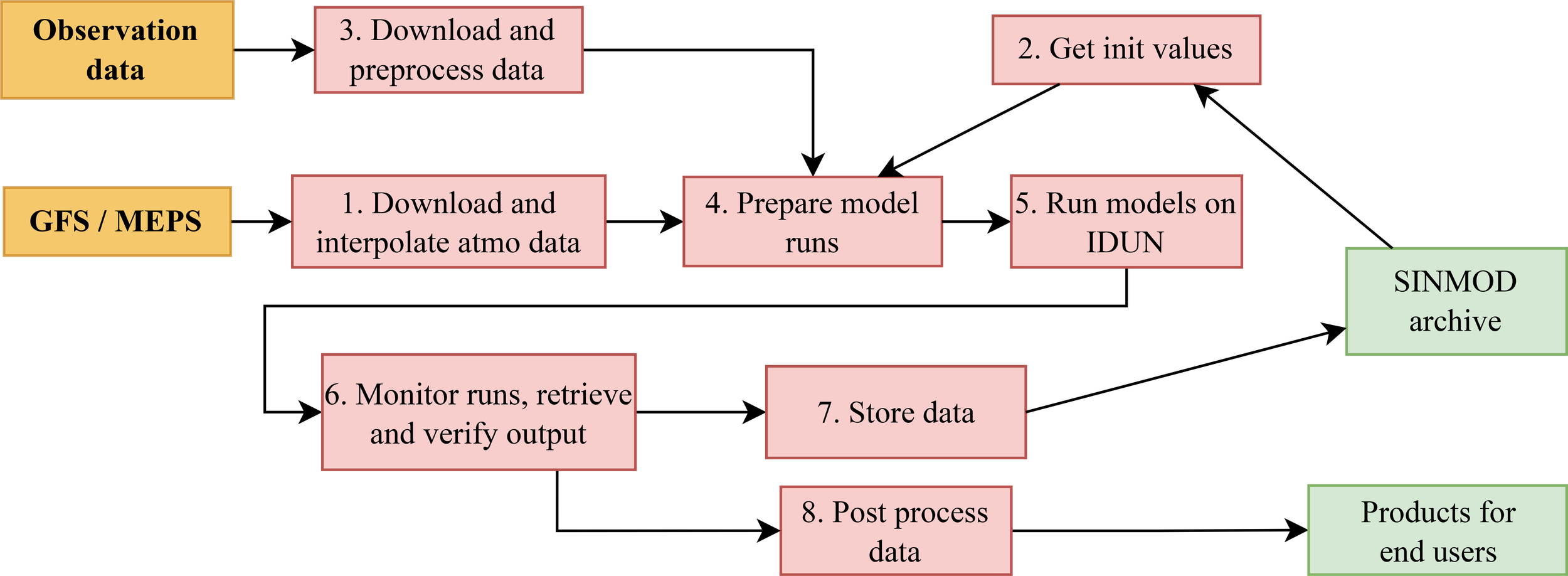
Schematic of the data flow in the operational model system.
-
Download atmospheric data for today’s run and interpolate it to the appropriate model grid.
-
Obtain initial values for physics and biology from that model run’s archive files (yesterday’s run provides the initial value for today’s run).
-
Download and preprocess data to be assimilated, if any.
-
Write settings files and job scripts and gather all necessary files for the model run.
-
Copy the files to NTNUs IDUN High Performance Computing (HPC) cluster (Själander et al., 2022) and initiate a batch job.
-
Monitor job execution, copy all output files back after the job is finished, check that the model has produced sufficient output and log an error message otherwise.
-
Archive state values for physics and biology 24 hours into the simulation for use as initial values.
-
Post-process and distribute model output.
Each individual model run was held off until its mother model had been running for a sufficiently long time (dependent on model run time). This ensured appropriate sequencing of model runs and that sufficient boundary values had been produced before nested models were started. As the model runs with data assimilation it requires a number of parallel nodes, and could potentially be held up in the queue. Six reserved compute nodes were used to avoid queue delays. The full system used approximately 5000 CPU hours per day. The daily model outputs were typically available between 05:00 and 09:00 local time, depending on the availability of atmospheric forcing data and the number of observations assimilated. The latter varied primarily with cloud cover conditions affecting satellite data retrieval.
3 Results and discussion
Following an initial verification phase, the observational platforms operated reliably within the integrated system. The timing of all gathered and assimilated data is illustrated in Figure 4.
Figure 4
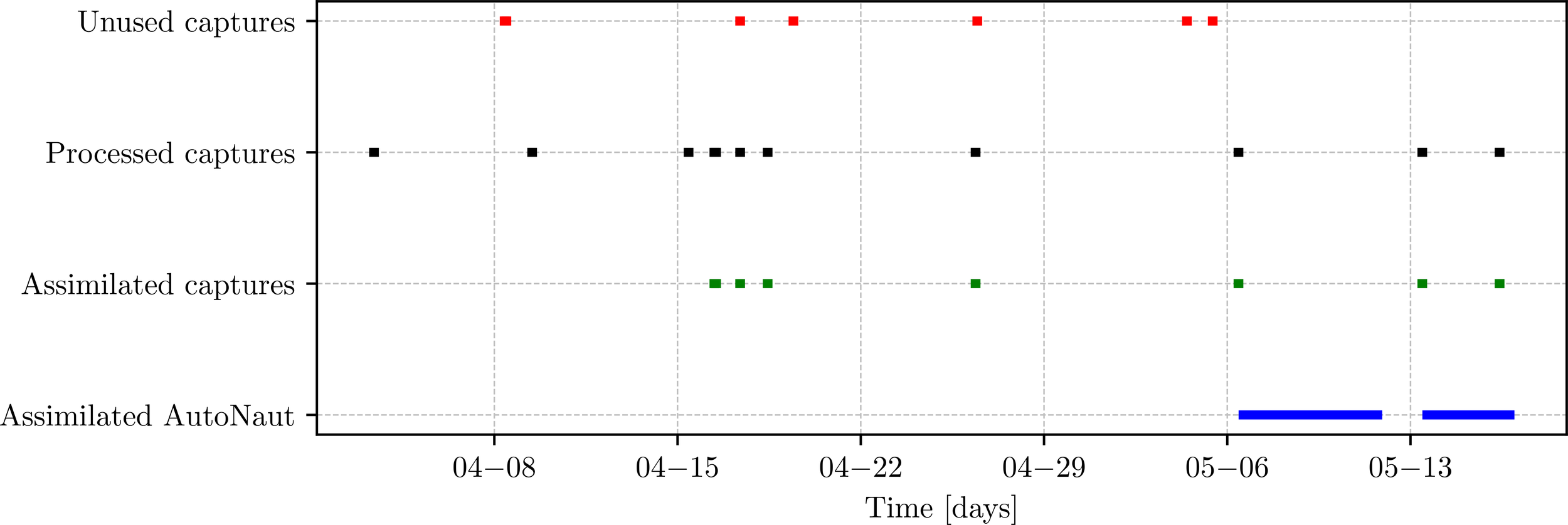
Timeline of collected data from the different sources in the observational campaign. The HYPSO1 data is separated into all captures that were processed, captures that were processed and assimilated and captures that were neither processed nor assimilated.
The following presents analysis of the campaign simulations and comparisons with the observational data. In addition to these analyses, post-field-campaign simulations are presented to address the model bias in Chl-a, focusing on the revised silicate model and updated Nitrogen-Carbon-Chlorophyll conversion factors within the ecosystem component of the ocean model. Additionally, the campaign identified several areas for improvement across various system components, including hardware limitations, software constraints, and communication challenges. These findings are detailed and discussed in the subsequent sections.
3.1 HYPSO-1 Chl-a estimate comparisons & model correction
During the observational campaign, a total of 20 HYPSO-1 captures were taken along the western- and mid-Norway coasts. Figure 5a displays the RGB renders of each hyperspectral capture. Because of processing latency and computational constraints, captures were eligible for assimilation only until midnight on the day of acquisition. Hence, only a subset of these captures were available for data assimilation in the aMIDNOR simulation. Specifically, eight captures were assimilated, with their RGB renders shown in Figure 5b and their timeline shown in Figure 4, with two captures taken on the 16th of April.
Figure 5
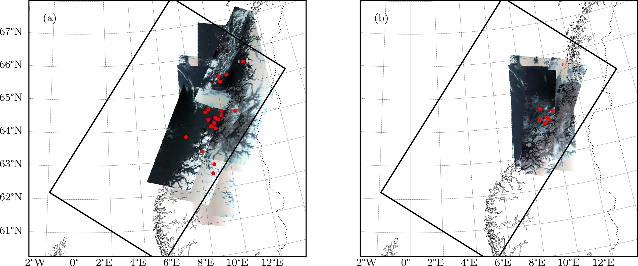
(a) HYPSO-1 RGB renders of the captures along the mid-Norway coast from April 2nd to May 21st, 2024. (b) HYPSO-1 RGB renders of the captures assimilated into the aMIDNOR operative simulation during the same period. A red point indicates the approximate center point of each capture.
A visual comparison of the HYPSO-1 Chl-a estimate (Figure 6a) with estimates from Sentinel-3 (Figure 6b), MODIS (Figure 6c), and the aMIDNOR simulation (Figure 6d) is presented for data from May 6th. HYPSO-1 data aligns more closely with MODIS near Frohavet, where MODIS shows higher Chl-a concentrations compared to Sentinel-3. Conversely, in the open ocean, MODIS generally exhibits lower Chl-a values than Sentinel-3. The aMIDNOR analysis overestimates coastal Chl-a except in areas directly constrained by HYPSO-1 observations.
Figure 6
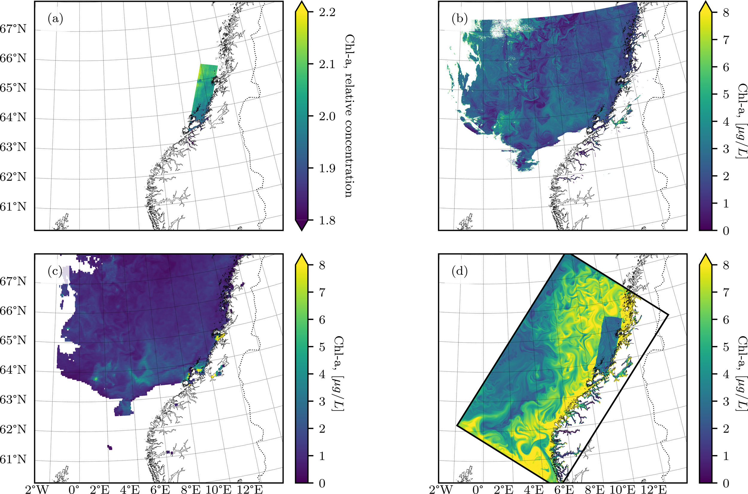
(a) HYPSO-1 Chl-a estimates from the May 6th 2024 10:17 UTC capture, (b) Sentinel-3 chlorophyll estimates from a May 6th 2024 10:20 UTC pass where Chl-a values greater than 7 are set to NaN, (c) MODIS Chl-a estimates from the May 6th 2024 pass, (d)aMIDNOR simulation Chl-a estimates.
The assimilation and propagation of corrections for the last three HYPSO-1 captures in the campaign are presented in Figure 7. The capture dates are May 6th (Figure 7a), May 13th (Figure 7d), and May 16th (Figure 7g). Additionally, the propagation of these corrections is shown after 24 hours (Figures 7b, e, h) for the respective captures) and after 48 hours (Figures 7c, f, i).
Figure 7
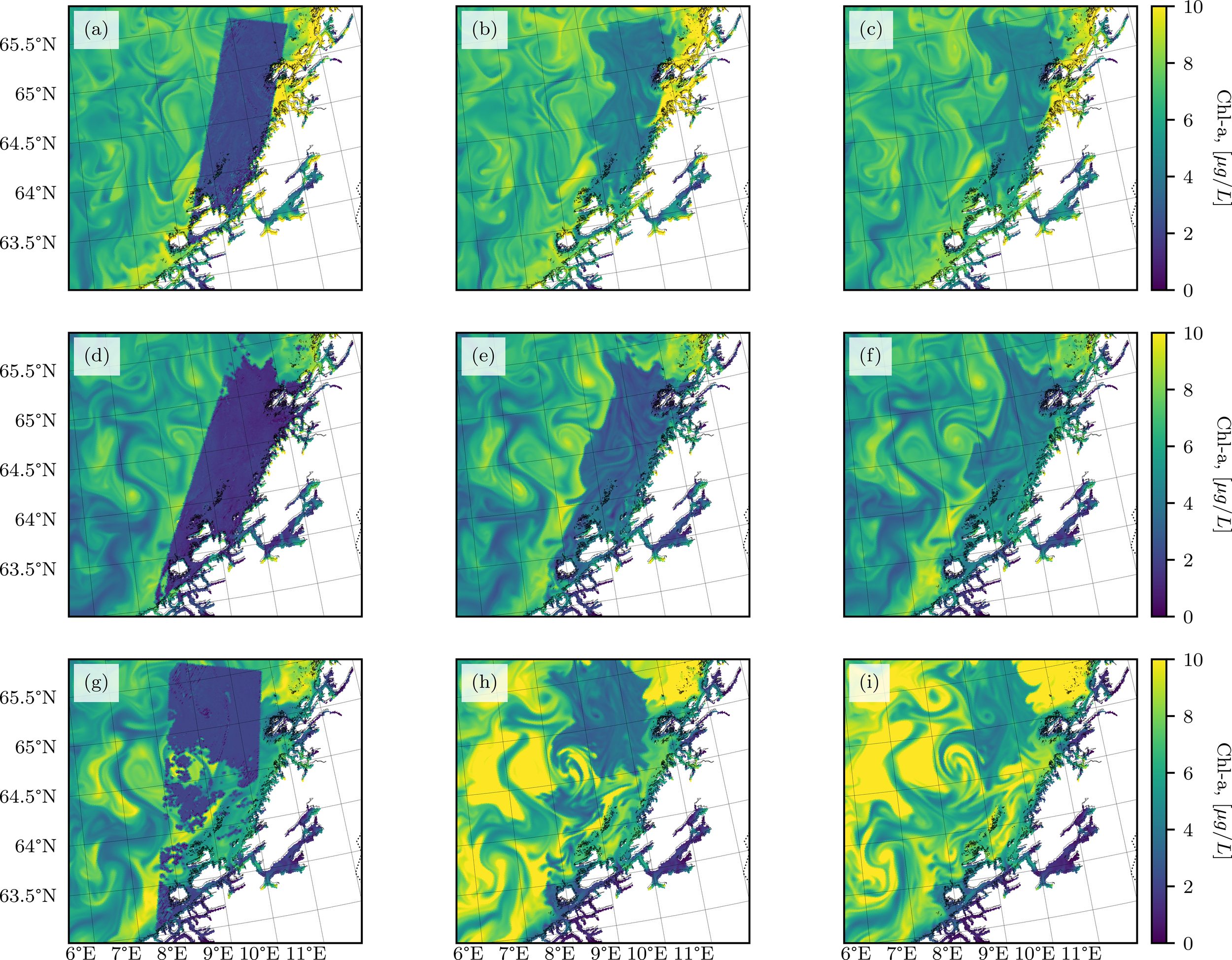
Chl-a estimates in the aMIDNOR simulation showing the propagation of HYPSO-1 observations. The first column (a, d, g) shows the assimilation days: (a) May 6th, (d) May 13th, (g) May 16th. The second column (b, e, h) shows one day after assimilation: (b) May 7th, (e) May 14th, (h) May 17th. The third column shows two days after assimilation: (c) May 8th, (f) May 15th, (i) May 18th.
The HYPSO-1 Chl-a estimates must be treated with high uncertainty, particularly in fjord regions where high colored dissolved organic matter (CDOM) can obscure Chl-a optical signatures, and more generally when strong particle backscattering alters the ocean-colour signal (e.g., during coccolithophore/PIC blooms). In such cases, enhanced particle backscattering violates the assumptions underlying standard band-ratio Chl-a algorithms, such that reflectance-derived Chl-a may become biased or inconsistent with true pigment concentrations (Oziel et al., 2017).
3.2 USV AutoNaut Chl-a observations & path planning
Daily optimal waypoints for the USV were computed using forecasts from the aFROSHELF simulation, employing the path planning algorithm detailed in Sec. 2.2.3.2 to identify high-priority areas and generate minimum-distance routes. The nitrate-related weighting in the cost function was set to zero for the first half of the campaign, as summarized in Table 2 for case 1. All remaining weights in the cost function were normalized according to Eq. 2. Optimized waypoint sets were implemented on May 10 and 14; on other days the USV followed previously computed or ad hoc waypoints due to operational constraints. An illustrative example is provided for May 10th (Figure 8), when forecasts were received at 09:40 CEST, waypoints were issued at 10:30 CEST, and the USV completed the target list between 12:00 and 24:00 CEST. Importantly, observational data from both the USV and the HYPSO-1 satellite were consistently assimilated into the ocean model throughout the campaign, irrespective of whether navigational paths followed optimal or arbitrary waypoints. This integrated approach demonstrates the closed-loop observational strategy, despite intermittent operational challenges.
Figure 8
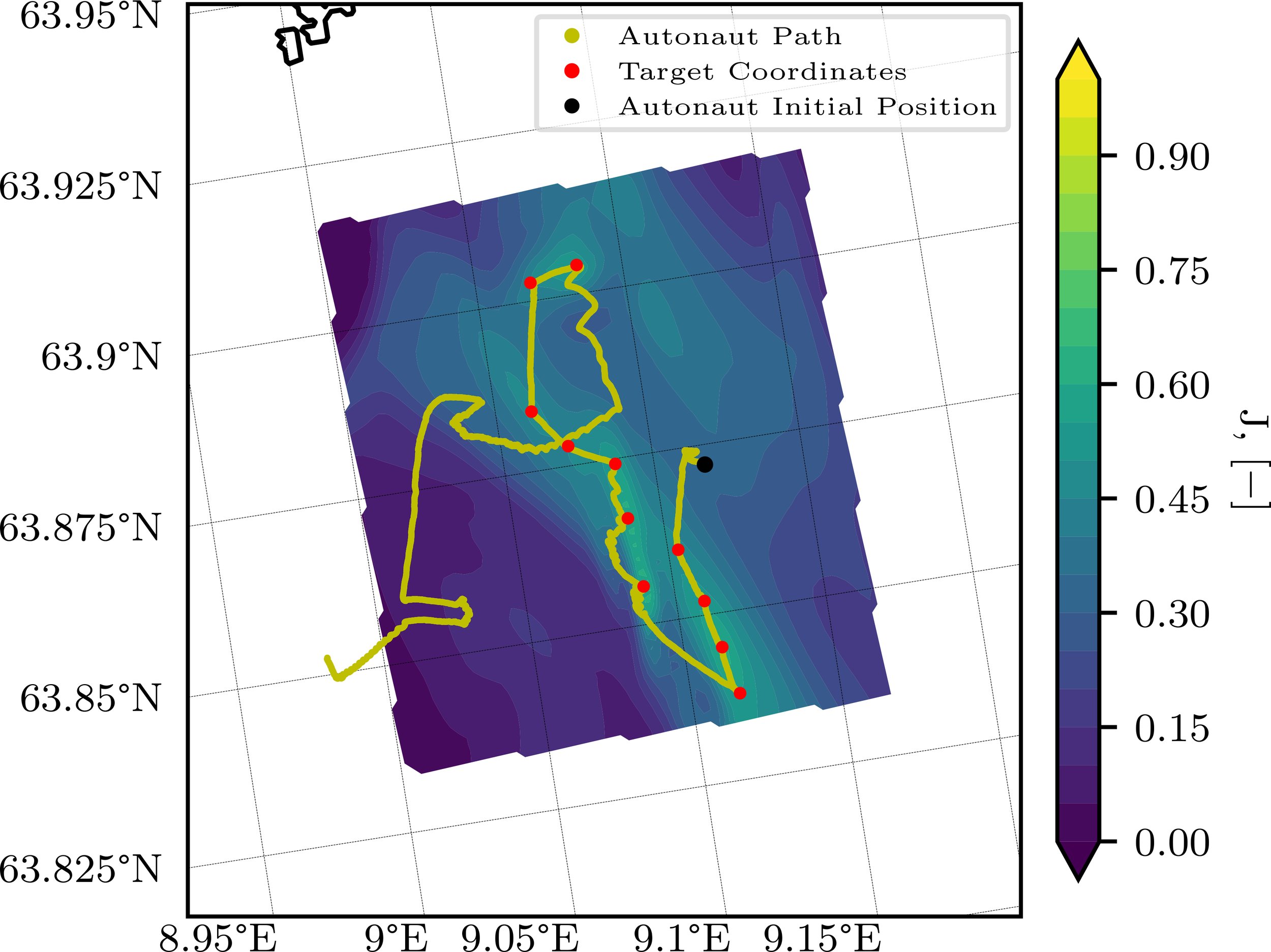
AutoNaut path in Frohavet on the 10th of May with the optimally chosen coordinates indicated in red. The computed score field, J is shown in the background.
Figure 9a shows the full path of the USV during its deployment period from the Mausund field station, out to Frohavet and back to the field station. The raw Chl-a observations from the USV are shown in Figure 9b, while Figure 9c displays the same observations post-processed with an NPQ correction method (Fragoso et al., 2024). As expected, the corrected observations exhibit slightly higher magnitudes, with a regional mean of 1.61 ± 0.47 µg/L. These values are consistent with Chl-a magnitudes derived from Sentinel-3 and HYPSO-1, but lower than those predicted by the FROSHELF simulation (Figure 9d). The Chl-a predictions from the aFROSHELF simulation, shown in Figure 9e, display lower values along and around the USV operational path, consistent with the assimilated observations indicating the model’s slight overestimation in this region. Finally, Figure 9f highlights the difference in predicted Chl-a levels between the FROSHELF and aFROSHELF simulations on May 11th (following the assimilation of May 10th observations). The red-shaded areas, particularly along the USV’s operational path, indicate a positive Chl-a bias in FROSHELF that is reduced in aFROSHELF through assimilation of the USV observations.
Figure 9
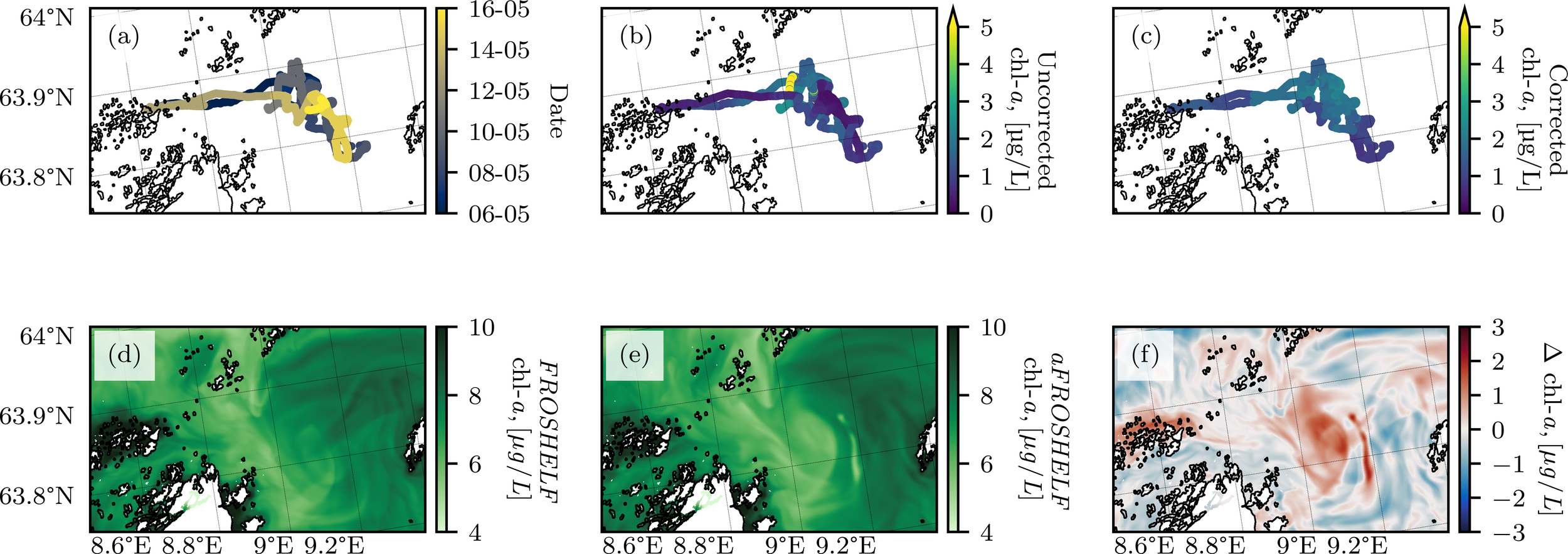
(a) AutoNaut observation path from 6th of May to 16th of May, 2024. (b) Observed Chl-a values without NPQ correction. (c) Observed Chl-a values with NPQ correction applied. (d) Simulated Chl-a values from the FROSHELF model on 11th of May. (e) Simulated Chl-a values from the aFROSHELF model on 11th of May. (f) Difference between FROSHELF and aFROSHELF Chl-a predictions on 11th of May.
Data from the aFROSHELF simulation were extracted at grid cells corresponding to the USV’s locations throughout the campaign period and averaged both over the model ensemble and within 6-hour time windows. The resulting mean and standard deviation are presented as error boxes alongside the Chl-a observations in the upper panel of Figure 10. The model data align well with the observations, though notable discrepancies arise following periods without USV observations, particularly on May 12th, when neither USV nor HYPSO-1 satellite observations were assimilated, effectively rendering the model run as open-loop. Ensemble spread, serving as an indicator of model uncertainty, was computed along the USV track. The lower panel of Figure 10 displays the 12-hour differences in ensemble spread, illustrating periods of reduced or increased forecast uncertainty. Optimal navigation periods (May 10th and 14th, highlighted in green) were specifically targeted toward regions of maximum ensemble spread, thereby anticipating notable reductions in spread, which is clearly demonstrated on May 10th. A significant reduction also occurs on May 14th; however, an even greater reduction observed on May 15th suggests additional factors, such as initially higher variance, may contribute to reductions in spread. Consequently, although optimal navigation clearly correlates with pronounced reductions in ensemble spread, a larger dataset comparing optimal and arbitrary navigation is necessary to robustly quantify the effectiveness of the closed-loop observational strategy.
Figure 10
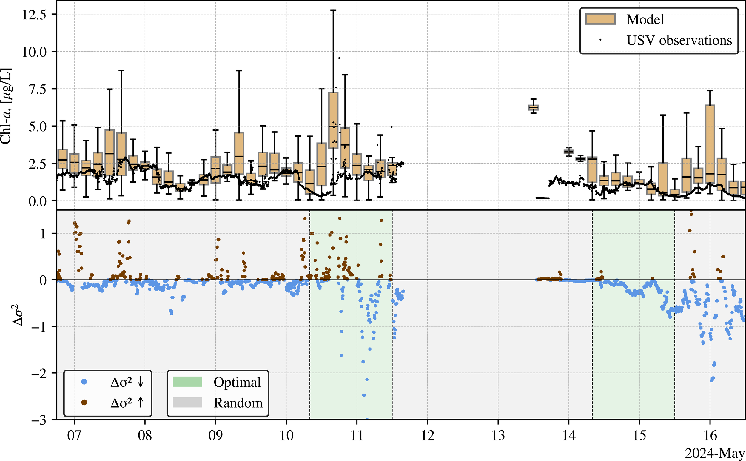
Upper panel: Comparison between Chl-a observations from the USV (black dots) and ensemble averaged model data (error boxes; mean ± standard deviation) extracted from the aFROSHELF simulation at corresponding USV locations. Lower panel: 12-hour difference in ensemble spread (Δσ2), indicating variance reduction (blue) or increase (brown). Optimal navigation days (May 10th and 14th) are highlighted in green; other days represent random or delayed waypoint implementation.
The closed-loop observation system was successfully demonstrated with a single USV, but a full-scale implementation aiming for higher accuracy and lower uncertainty would likely require multiple USVs. Multiple platforms would enhance spatial and temporal coverage and reduce limitations of a single-USV setup, such as restricted area coverage, low revisit frequency, and vulnerability to navigation or communication failures. Because observations were limited to the surface layer in a highly variable region, some corrections may redistribute vertically through mixing, allowing subsurface water masses, less constrained by surface data depending on the ensemble’s vertical covariances and localization scales, to influence surface conditions. Including an underwater vehicle alongside the USV would provide valuable subsurface observations.
During initial tuning, the horizontal localization length was reduced from 1000 m to 300 m to mitigate sampling noise associated with the limited ensemble size, which stabilized corrections in the diatom and flagellate fields.
The experiment also revealed areas for improvement in the perturbation and uncertainty treatment of the diatom, flagellate, and nutrient fields. Because the ensemble spread was used as a direct measure of model uncertainty, no covariance inflation was applied, meaning that ensemble variability was maintained solely through the applied perturbations. In regions without direct USV observations, this occasionally resulted in excessive ensemble spread despite balanced perturbations scaled to the region’s natural variability through EOFs. Subsequent tests indicate that moderate covariance inflation improves stability and robustness, although it decouples ensemble spread from a strict uncertainty metric.
3.3 Operational challenges & limitations
End-to-end latency from observation to tasking depended on software throughput, communication, computational budget, and environmental conditions. Each of these elements can introduce delays that affect the overall timeliness of the integrated system. Some of the operational tasks requiring human interaction or input are listed in Table 4. Latency due to human communication (e-mail or similar) is not listed. Processing of model data is not listed as this was automated.
Table 4
| Task | HYPSO-1 capture & downlink | HYPSO-1 processing | USV grafana | USV neptus/dune | USV path planning |
|---|---|---|---|---|---|
| Latency | 2 hrs | 40–70 min | 5–10 min | 30–60 min | 10–30 min |
Time (typically) spent on retrieval or processing of observations from HYPSO-1 and the USV.
The efficiency of this closed-loop approach is influenced by physical limitations. For instance, cloud coverage or solar storms can disrupt satellite operations, while harsh weather conditions can impact the navigational performance of the USV, preventing it from reaching planned coordinates (Baker, 2001; Liu et al., 2016; Dubovik et al., 2021). These environmental challenges highlight the need for robust contingency planning to maintain system performance.
Mid-campaign and post-campaign assessments of the performance and latency of the USV, satellite and operational model involved in the field campaign revealed various challenges and limitations, each introducing minor to moderate delays that affect the overall efficiency and timeliness of the integrated system. These issues highlight the need for improved synergy and clear problem descriptions among subsystems. Addressing these challenges is crucial for future observational campaigns to enhance planning related to HPC budget, personnel, and observational capabilities. Future campaigns should employ a multi-layer modeling tool to map requirements, describe functionalities, and simulate agent planning and data assimilation, thereby enhancing overall system coordination and performance. Below are key points highlighting some of these challenges and limitations.
3.3.1 Model limitations
As detailed in Sec. 2.4, the model setup’s required forcing inputs were automated, leaving the computational budget as the primary limitation. With 336 CPUs available for 12 hours each day, resources had to be allocated to either increase model simulation speed via OpenMP parallelization or enhance the statistical basis for the EnKF algorithm’s background error covariance matrix by increasing the number of ensemble members. To maintain a 48-hour forecast, the assimilation window for observations was limited to 24 hours before the simulation started at midnight for the aMIDNOR and aFROSHELF simulations. A larger computational budget could extend the observational window, improve the covariance structure, and enhance predictive capability, depending on the availability of forcing conditions like atmospheric inputs. With additional resources, the state vector could also be expanded to include key nutrients so that EnKF updates exploit covariances between phytoplankton and nutrient fields. Such an extension would require larger ensembles and carefully designed perturbations to avoid spurious cross-variable updates, and its benefit depends on whether the background-error covariances capture the expected anti-correlations between biomass and nutrients.
Regarding the propagation of uncertainty from aGIN through aNOR4KM, aMIDNOR, and aFROSHELF: while each simulation displays an ensemble spread, the boundary conditions are defined by the ensemble mean, resulting in single-value boundaries. This lack of ensemble information at the boundaries is propagated through the nested simulations. Consequently, even though there is uncertainty within each nested model domain, the boundary conditions are assigned with 100% accuracy due to averaging, which results in a loss of ensemble spread which eliminates uncertainty at the boundaries. As a result, observations in these regions exert minimal influence. Storing the boundaries for each ensemble member individually could address this issue, potentially increasing the ensemble spread and enhancing the covariance structure in nested model setups.
As described in Secs. 3.1 and 3.2, the model, employing the fixed carbon:nitrogen:Chl-a conversion factors outlined in Sec. 2.1.4, overestimates Chl-a concentrations compared to observations from the HYPSO-1, MODIS, and Sentinel-3 satellites, as well as in situ measurements from the USV. This overestimation suggests either an inaccurate conversion of phytoplankton biomass to Chl-a or excessive phytoplankton biomass in the model. Overestimation of nutrient concentrations, such as nitrate and silicate, can lead to excessive primary production. Such biases may arise from inaccuracies in key processes such as vertical mixing, remineralization, or nutrient recycling. Additionally, underestimated zooplankton concentrations in the model may reduce grazing pressure and contribute to elevated phytoplankton biomass. More generally, the structure of the biological model itself represents an additional source of uncertainty, as the ecosystem configuration resolves only diatoms and a generic flagellate group and therefore does not explicitly represent other emerging phytoplankton functional types (e.g. coccolithophores). Such groups can substantially modify the optical properties of the water column and thereby affect the interpretation of ocean-color–derived Chl-a observations, which in turn may influence the corrections applied to the model state through data assimilation. These groups are most relevant during summer to late-summer stratified conditions in Atlantic-influenced waters (Oziel et al., 2017; Neukermans et al., 2018).
Post-field campaign analyses of the operational model revealed persistently high silicate concentrations along the Norwegian coast throughout the spring bloom, suggesting insufficient silicate depletion in the model contributing to prolonged primary production and elevated Chl-a values. In response to these issues, the silicate dynamics of the ocean model (Sec. 2.1.4) were updated by adding previously absent vertical and horizontal advection of rapidly sinking silicate detritus and relocating a production term for silicate detritus from microzooplankton grazing on diatoms into rapidly sinking detritus. A new set of simulations was performed to evaluate the revised silicate model. Differences in silicate and nitrate levels for the surface layer, spatially averaged over the Frohavet region, are shown in the upper panel of Figure 11. In the early spring, silicate levels in the two model versions are similar, while by April the reworked model shows faster silicate depletion. Chl-a levels are shown in the bottom panel of Figure 11, where the dashed black line displays the original MIDNOR freerun simulation with the silicate model utilized in the operational field campaign, and the solid black line without uncertainty shading displays the MIDNOR data from a simulation using the reworked silicate model. The reworked model predicts initially elevated Chl-a concentrations during the early bloom but aligns more closely with observed values by late April.
Figure 11
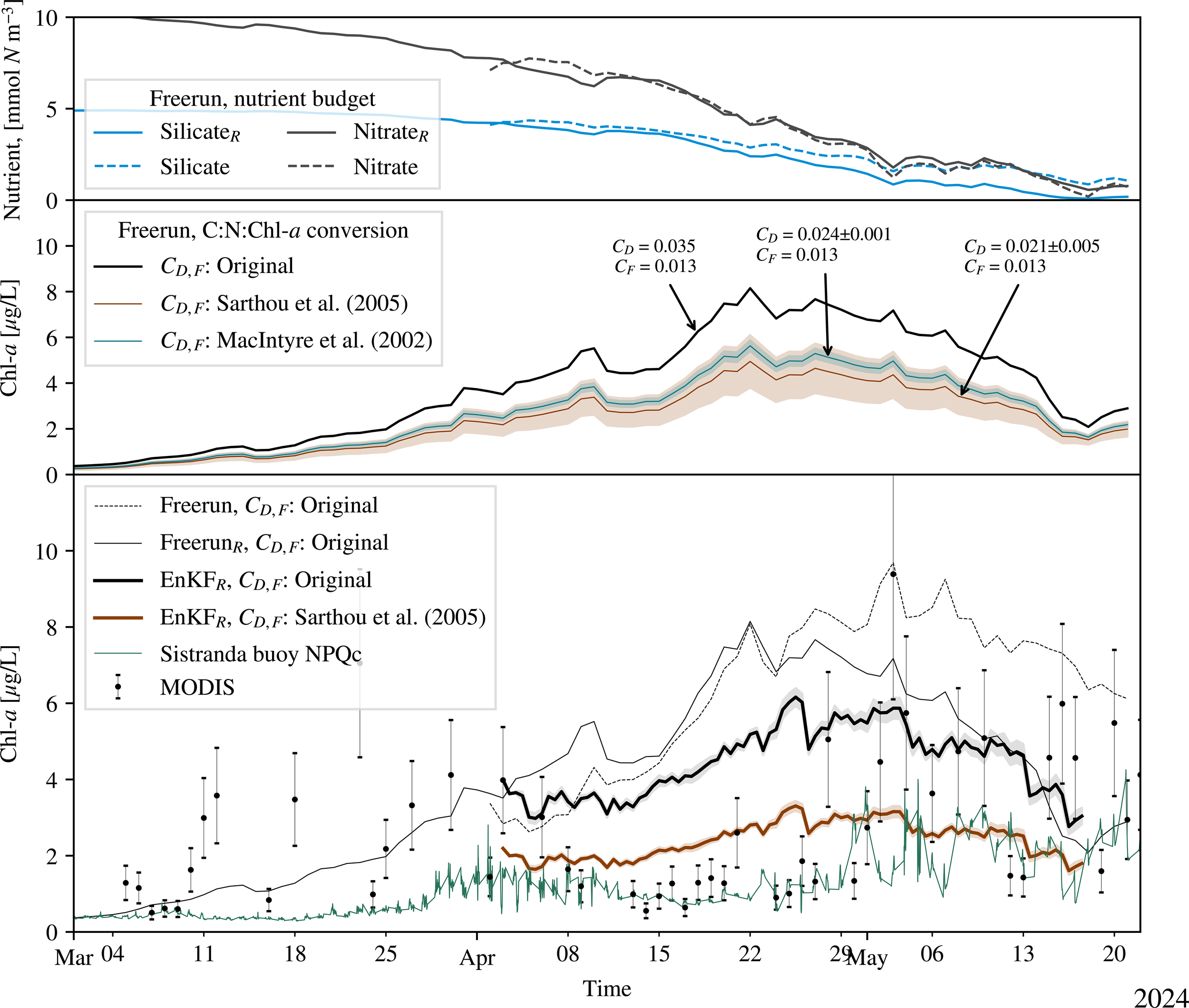
Post–field-campaign ecosystem-bias analysis for the MIDNOR domain in the Frohavet region. Upper panel: Spatially averaged surface silicate and nitrate comparing the original and reworked nutrient budgets. Middle panel: Sensitivity of modeled surface Chl-a to C:N:Chl-a conversion factors under the reworked nutrient budget. Curves show the field-campaign factors and literature values from MacIntyre et al. (2002) and Sarthou et al. (2005). Shaded envelopes indicate the reported uncertainty ranges. Lower panel: Spatially averaged surface Chl-a time series. Lower panel: Spatially averaged surface chlorophyll-a time series. Shown are (i) freerun, original budget (black dashed), (ii) freerun, reworked budget (black thin solid), (iii) EnKF, reworked budget with field-campaign factors (black thick solid; gray band = ensemble spread), and (iv) EnKF, reworked budget with Sarthou et al. (2005) factors (brown thick solid). Observations are the Sistranda buoy (NPQ-corrected; green line) and MODIS (black points with ±35% error bars).
Figure 11 compares modeled Chl-a to two independent observation sources: in situ buoy data at Sistranda, Frøya, located in southern Frohavet (see Figure 1), and spatially averaged MODIS Chl-a data for the Frohavet region. The buoy observations, collected from February to June 2024, were corrected for NPQ using the same method applied to the USV data. The MODIS Chl-a data, spatially averaged over the Frohavet region, are shown with a ±35% error margin, based on the uncertainty estimate from Moore et al. (2009). The modeled Chl-a concentrations, both for the original and revised simulations, generally fall within the error range of the MODIS data, except for a notable discrepancy in mid-April. However, the initial silicate levels in the simulations may still be overestimated.
Another potential source of error is the use of fixed carbon:nitrogen:Chl-a conversion factors, as described in Sec. 2.1.4. Fixed factors can lead to over- or underestimation depending on variations in sunlight, nutrient availability, and temperature (MacIntyre et al., 2002; Sarthou et al., 2005; Lacour et al., 2017). In particular, phytoplankton pigment content varies with irradiance conditions with higher irradiance typically leading to lower conversion factors. A simplified sensitivity analysis was conducted for the spatially averaged surface MIDNOR data, examining how varying carbon-to-Chl-a conversion factors for diatoms and flagellates influence Chl-a estimates. The results, shown in the middle panel of Figure 11, compare the original predictions with those obtained using modified conversion factors. Since diatoms dominate during the spring bloom in Norwegian coastal waters, the conversion factor for diatoms, CD, was altered the most, ranging from 0.02 to 0.035. Empirical values for polar diatoms are reported as 0.035 ± 0.005, gC, g−1Chl-a by Lacour et al. (2017), 0.021 ± 0.005, gC, g−1Chl-a by Sarthou et al. (2005), and 0.024 ± 0.001, gC, g−1Chl-a by MacIntyre et al. (2002). Findings from the sub-polar Labrador Sea, which may be more representative of our study region’s conditions, show lower carbon-to-Chl-a factors (ranging between 0.007 and 0.02, gC, g−1Chl-a) under diatom-rich scenarios (Fragoso et al., 2017a; Fragoso et al., 2017b), suggesting that even lower conversion factors could be appropriate for our sub-polar setting.
While the adjusted lower conversion factors bring modeled Chl-a closer to the Sistranda buoy observations, there is still a slight overestimation compared to MODIS data. Moreover, even with refined conversion factors, the modeled seasonal progression of Chl-a remains inconsistent with observed patterns. This suggests that variable, dynamically adjusted conversion factors or incorporating a fully interactive Chl-a model within the ecosystem component may be necessary to better capture the regional variability and improve overall model performance.
An additional EnKF simulation was conducted using the reworked silicate model and assimilating all available HYPSO-1 observations (20 captures). The results, shown as the solid black line with uncertainty shading in the lower panel of Figure 11, demonstrate improved agreement with in situ Sistranda buoy data and MODIS satellite observations during mid-April, surpassing the performance of both the original and reworked freerun simulations. Moreover, the reworked silicate model was combined with conversion factors from Sarthou et al. (2005) (CD = 0.021 ± 0.005, gC, g−1Chl-a). As shown by the solid brown line in Figure 11, this configuration yields a closer match to both MODIS data and the Sistranda buoy records. A longer spin-up spanning at least one seasonal cycle would permit the revised silicate dynamics to equilibrate with circulation and biology, likely lowering pre-bloom silicate and improving agreement with observed Chl-a.
Figure 12 contrasts the field-campaign operational configuration and the post-campaign analysis. Panels (a–c) show the MIDNOR simulation used during the field campaign (no data assimilation in this time window due operational latency), with the field-campaign nutrient budget and C:Chl-a factors. Panels (d–f) show the post-campaign configuration (aMIDNOR) with the reworked silicate budget and the C:Chl-a conversion from Sarthou et al. (2005). Across the domain, Chl-a concentrations are markedly lower in (d–f) than in (a–c), consistent with the combined effects of reduced silicate availability and the revised conversion factors. On April 8, the HYPSO-1 scene appears as a dark, rectangular imprint around Frøya and Hitra; by April 9–10 this signal is advected and deformed by alongshore currents and circulation in Frohavet, yielding spatial structures more consistent with observations and improving upon the results in Sec. 3.1.
Figure 12
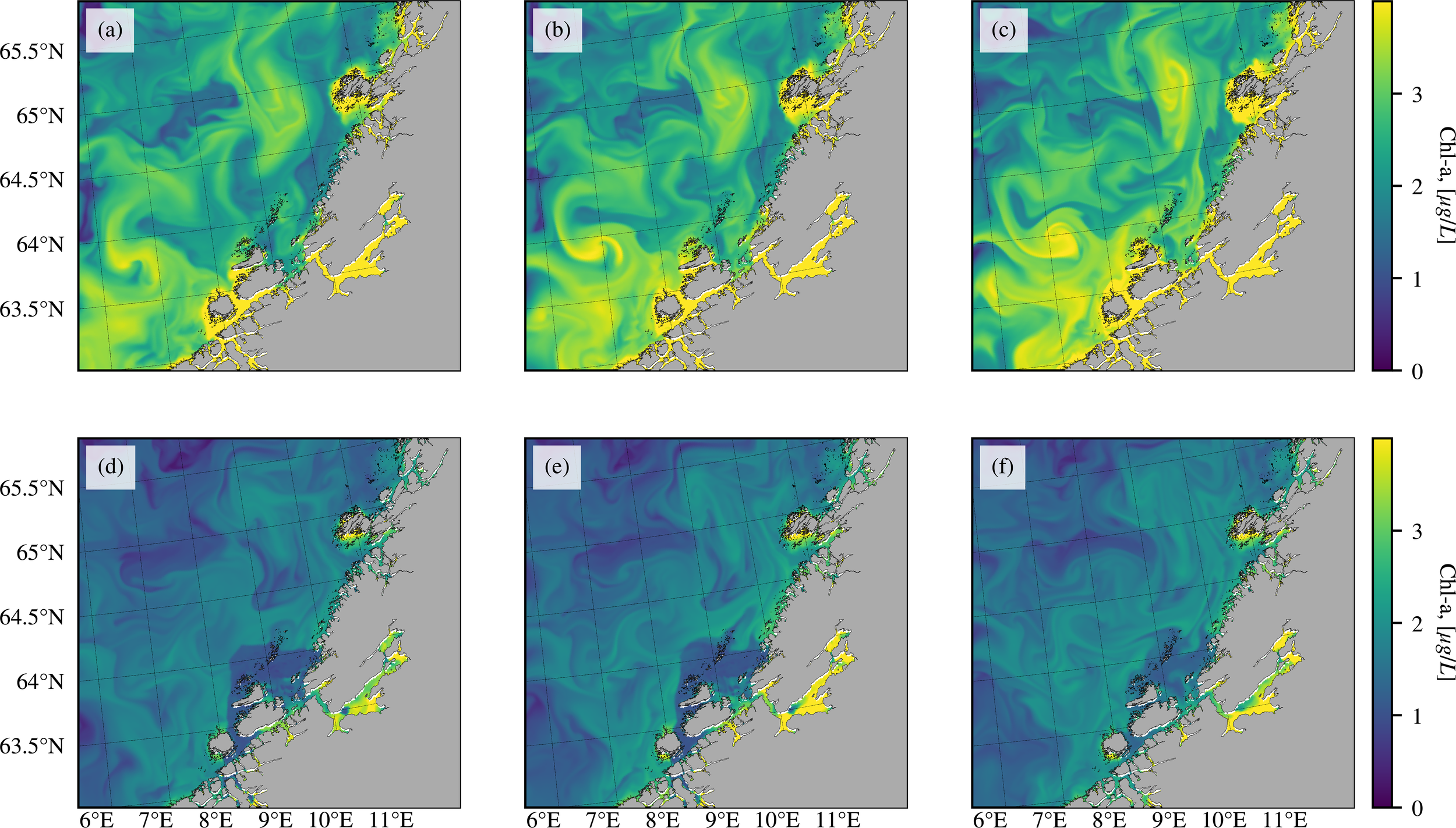
Chl-a fields for April 8–10. (a–c) show the MIDNOR simulation in the fieldcampaign operational configuration (no data assimilation), using the field-campaign nutrient budget and C:Chl-a factors, on April 8, 9, and 10. (d–f) show the post-campaign analysis configuration (aMIDNOR) using the reworked silicate model and the C:Chl-a conversion from Sarthou et al. (2005)CD = 0.021 ± 0.005 gCg−1 Chl-a, illustrating the propagation of the HYPSO-1 capture over April 8–10.
In the current framework, path planning is informed by forecasted chl-a gradients/fronts and by ensemble variance. As such, correcting a mean model bias is expected to have limited direct impact on route geometry, because the planner primarily responds to spatial structure rather than absolute levels. The more relevant impact of bias correction is indirect. Reducing systematic observation–model residuals decreases analysis increments and improves filter consistency/reliability of the ensemble spread that the planner uses. Consequently, bias correction should stabilize waypoint prioritization (fewer aggressive re-plans) rather than fundamentally change the route, with the largest benefits when bias distorts bloom timing/magnitude enough to alter gradient placement.
3.3.2 HYPSO-1 challenges & limitation
The primary challenge with the HYPSO-1 satellite was cloud coverage, which limited the usefulness of captures for Chl-a estimates to a few times per week, despite a capacity of up to two daily captures along the Norwegian coast at this time of season.
Additionally, space weather forecasts, provided by the National Oceanic and Atmospheric Administration (NOAA) (NOAA, 2024), necessitated powering down non-essential subsystems of the satellite to prevent radiation damage. Several space weather parameters are monitored, such as the geomagnetic storm classification (G-class or alternatively the KP-index), proton flux and solar magnetic winds. With a KP-index (which is a measure of the geomagnetic activity) above 5, the payload controller as well as the payload itself were powered off. During the observation campaign, a series of powerful solar storms with extreme solar flares and geomagnetic storm components occurred from 10th–13th of May 2024 during solar cycle 25 (Karan et al., 2024). The geomagnetic storm was classified as a G5-class, being the most intense storm since 2003 (Mannucci et al., 2005). This led to multiple periods where satellite operations were prohibited. Specifically on the night of April 4th-5th, the evening of April 14th, the morning of May 6th, the afternoon of May 10th until the morning of May 13th, early morning and afternoon/evening of May 14th, and midday on May 20th.
Absence of downlink prioritisation occasionally delayed processing beyond the assimilation window. Implementing a priority logic would indeed help in respecting the time requirements. This issue could likely have been mitigated through improved logistical planning.
Although the HYPSO-1 satellite had been operational for over two years, its near-real-time capabilities had been tested but not operationally implemented. Several critical tasks required human intervention, such as data processing, indirect georeferencing, and generating cloud masks. The one-day observational window imposed by the low computational budget meant that not all captures over targeted areas were ready for data assimilation due to the high human involvement and limited automation. Increasing the computational budget and implementing an improved data pipeline with an API could increase the chances of captures being available for assimilation. In preparation for future field campaigns, some processing steps were automated based on challenges identified in this deployment. E.g. georeferencing was migrated from a manual workflow to an automated procedure to improve consistency and shorten turnaround from downlink to analysis.
3.3.3 AutoNaut challenges & limitations
The AutoNaut deployment, initially scheduled for April 2nd to April 30th, 2024, was delayed due to hardware installation that included sensor integration and further testing. The USV operated from 6th to 16th of May with a brief interruption on May 12th.
In Frohavet, the AutoNaut faced varying weather conditions from calm waters to moderate waves and heavy winds. Operators had to monitor forecasts and retrieve the vehicle if necessary. Despite the predefined operational area being low in commercial shipping traffic, operators also needed to monitor the USV’s path to avoid deviations that could lead to interference with commercial vessels due to hardware malfunctions or strong winds.
Despite the possibility of monitoring remotely the collected data, the IoT (internet of things) architecture lacked an automatic data retrieval method. Initially, Chl-a data was obtained as.csv files downloaded via the Grafana interface. However, as this method depends on cellular network coverage, a discontinuous data flow was observed due to occasional poor connections in Frohavet. On May 15th, the operational system was changed to retrieve observational data by downloading log files directly from the USV, reducing data transfer to onshore servers and Grafana and therefore possible losses due to bad coverage. These logs were then processed using the Neptus interface, providing a complete dataset for state feedback in the closed-loop system. The observational data was processed in Python to obtain 5-min averages before being sent for assimilation into the ocean model. USV coordinates from the optimal path planner, detailed in Sec. 2.2.2, had to be manually sent to operators, who created and uploaded new missions to the USV, introducing latency in the communication and task execution process.
Opportunities for automation were identified but not implemented during this campaign. Planned improvements include scripted retrieval of log files and telemetry from Neptus/DUNE, automated preprocessing of chl-a time series (filtering and aggregation to analysis intervals), and standardized formatting for model assimilation. Similar automation is envisaged for path-planning, with generation of optimal waypoints immediately after model forecasts are available and automatic upload of new missions to the USV via the Neptus/DUNE interface, thereby removing manual handover. Together, these steps are expected to reduce manual workload and shorten the observation-to-decision cycle in future field campaigns.
4 Conclusion
We present the first field-campaign demonstration of a closed-loop coastal-ocean observing system integrating low-Earth-orbit hyperspectral sensing, autonomous surface vehicles, and a high-resolution operational ocean model within a unified state-feedback framework. Chlorophyll-a estimates from the agile CubeSat HYPSO-1 and in-situ measurements from a wave-propelled AutoNaut USV were assimilated using an Ensemble Kalman Filter, with each analysis directly informing adaptive waypoint optimisation for the USV. Although dynamic retargeting for HYPSO-1 was planned, persistent cloud cover over the Norwegian coast necessitated a fallback to predetermined satellite capture targets.
The operational system demonstrated effective performance within available resources, successfully correcting model forecasts towards observational values across all computational domains. This facilitated accurate tracking of the seasonal algal bloom. Nonetheless, the campaign revealed several critical areas for improvement. Initial delays in HYPSO-1 data downlink and processing temporarily compromised forecast accuracy due to limited observational input, though iterative updates in the system integration alleviated this issue throughout the campaign. Persistent regional cloud cover limited satellite target planning, highlighting the importance of incorporating robust contingency planning. Furthermore, ecosystem-model biases arising from simplified silicate dynamics and fixed carbon nitrogen Chl-a ratios were identified and addressed in post-campaign analyses.
Despite these challenges, the successful operational integration of smart, adaptive observational platforms with an operational ocean model demonstrates the feasibility and potential of closed-loop ocean observing systems. Future enhancements, including advanced sensor technologies, automated data workflows, and tighter multi-platform integration, will build upon this proof-of-concept, enabling more responsive, accurate, and efficient ocean monitoring across multiple spatial and temporal scales.
Statements
Data availability statement
The raw data supporting the conclusions of this article will be made available by the authors, without undue reservation.
Author contributions
DH: Project administration, Data curation, Validation, Formal Analysis, Visualization, Methodology, Software, Conceptualization, Writing – review & editing, Writing – original draft, Investigation. CC: Investigation, Software, Conceptualization, Writing – review & editing, Visualization, Data curation, Formal analysis, Writing – original draft, Validation, Methodology. CP: Visualization, Conceptualization, Investigation, Validation, Formal analysis, Methodology, Writing – review & editing, Writing – original draft, Data curation, Software. AS: Validation, Conceptualization, Data curation, Writing – review & editing, Methodology, Writing – original draft, Investigation, Visualization, Formal analysis, Software. SB: Writing – review & editing, Project administration, Writing – original draft, Methodology, Investigation, Data curation, Software, Resources, Conceptualization. GF: Formal analysis, Supervision, Writing – review & editing, Data curation, Resources, Methodology, Writing – original draft, Conceptualization, Investigation, Funding acquisition. RB: Supervision, Resources, Funding acquisition, Data curation, Writing – original draft, Project administration, Writing – review & editing, Methodology. AD: Software, Methodology, Writing – review & editing, Writing – original draft, Data curation, Resources. JG: Resources, Conceptualization, Project administration, Methodology, Writing – review & editing, Data curation, Software, Writing – original draft. TJ: Methodology, Writing – original draft, Resources, Project administration, Conceptualization, Funding acquisition, Writing – review & editing, Supervision. IE: Validation, Methodology, Formal analysis, Supervision, Writing – review & editing, Software, Writing – original draft, Resources, Investigation. MA: Visualization, Formal analysis, Validation, Resources, Data curation, Supervision, Conceptualization, Writing – review & editing, Software, Methodology, Writing – original draft, Investigation.
Funding
The author(s) declared that financial support was received for this work and/or its publication. This work was funded by the Research Council of Norway through the HYPSCI (grant number 325961), ARIEL (grant number 333229), MoniTARE (grant number 315514) and Green Platform (grant number 328674), as well as the European Commission through the DiverSea project (grant number 101082004), and internally by the Norwegian University of Science and Technology.
Acknowledgments
We appreciate the daily reservation of 6 nodes on the IDUN HPC cluster, managed by NTNU IT, which enabled us to perform the simulations operationally. This study has been conducted using E.U. Copernicus Marine Service Information; https://doi.org/10.48670/moi-00165. We acknowledge the contributions of the AutoNaut team with Morten Einarsve, Pål Kvaløy, Glenn Angell and Pavel Skipenes, as well as the staff at Mausund Field Station for their assistance in the deployment and retrieval of the AutoNaut.
Conflict of interest
The authors declare that the research was conducted in the absence of any commercial or financial relationships that could be construed as a potential conflict of interest.
Generative AI statement
The author(s) declared that generative AI was not used in the creation of this manuscript.
Any alternative text (alt text) provided alongside figures in this article has been generated by Frontiers with the support of artificial intelligence and reasonable efforts have been made to ensure accuracy, including review by the authors wherever possible. If you identify any issues, please contact us.
Publisher’s note
All claims expressed in this article are solely those of the authors and do not necessarily represent those of their affiliated organizations, or those of the publisher, the editors and the reviewers. Any product that may be evaluated in this article, or claim that may be made by its manufacturer, is not guaranteed or endorsed by the publisher.
Footnotes
1.^ https://www.emc.ncep.noaa.gov/emc/pages/numerical_forecast_systems/gfs.php
2.^ https://thredds.met.no/thredds/catalog/mepslatest/catalog.html
3.^6U refers to six units (U), each measuring 10×10×10cm. HYPSO-1 measures 10×20×30cm
4.^ https://github.com/NTNU-SmallSat-Lab/hypso-package
5.^ https://www.seabird.com/eco-triplet-w/product?id=60762467721
6.^ https://www.seabird.com/sbe-49-fastcat-ctd/product?id=60762467704
References
1
Applegate D. Bixby R. Chvátal V. Cook W. (2006). The traveling salesman problem: A computational study ( Princeton University Press). Available online at: https://www.researchgate.net/publication/268645053_The_Traveling_Salesman_Problem_A_Computational_Study/citations.
2
Baker D. N. (2001). “ Satellite anomalies due to space storms,” in Space storms and space weather hazards. NATO Science Series, vol 38. ed. DaglisI. A. (Dordrecht: Springer). doi: 10.1007/978-94-010-0983-611
3
Bakken S. Henriksen M. B. Birkeland R. Langer D. D. Oudijk A. E. Berg S. et al . (2023). HYPSO-1 cubeSat: first images and in-orbit characterization. Remote Sens.15, 755. doi: 10.3390/rs15030755
4
Bates N. R. Astor Y. M. Church M. J. Currie K. Dore J. E. González-Dávila M. et al . (2014). A time-series view of changing surface ocean chemistry due to ocean uptake of anthropogenic CO and ocean acidification. Oceanography27, 126–141. doi: 10.5670/oceanog.2014.16
5
Behrenfeld M. J. Boss E. S. (2014). Resurrecting the ecological underpinnings of ocean plankton blooms. Annu. Rev. Mar. Sci.6, 167–194. doi: 10.1146/annurev-marine-052913-021325
6
Beldring S. Engeland K. Roald L. A. Sælthun N. R. Voksø A. (2003). Estimation of parameters in a distributed precipitation-runoff model for Norway. Hydrology Earth System Sci.7, 304–316. doi: 10.5194/hess-7-304-2003
7
Berget G. E. Eidsvik J. Alver M. O. Johansen T. A. (2023). Dynamic stochastic modeling for adaptive sampling of environmental variables using an AUV. Autonomous Robots47, 483–502. doi: 10.1007/s10514-023-10095-8
8
Berget G. E. Eidsvik J. Alver M. O. Py F. Grøtli E. I. Johansen T. A. (2022). “ Adaptive underwater robotic sampling of dispersal dynamics in the coastal ocean,” in Robotics research. Eds. AsfourT.YoshidaE.ParkJ.ChristensenH.KhatibO. ( Springer International Publishing, Cham), 610–625. doi: 10.1007/978-3-030-95459-837
9
Berget G. E. Fossum T. O. Johansen T. A. Eidsvik J. Rajan K. (2018). Adaptive sampling of ocean processes using an AUV with a gaussian proxy model. ( IFAC-PapersOnLine 51), 238–243. doi: 10.1016/j.ifacol.2018.09.509
10
Bjornsson H. Venegas S. A. (1997). A manual for EOF and SVD analyses of climate data. Tech. Rep.
11
Brunet C. Johnsen G. Lavaud J. Roy S. (2011). “ Pigments and photoacclimation processes,” in Phytoplankton pigments: characterization, chemotaxonomy and applications in oceanography. Eds. LlewellynC. A.EgelandE. S.JohnsenG.RoyS. ( Cambridge University Press, Cambridge), 445–471. Cambridge Environmental Chemistry Series. doi: 10.1017/CBO9780511732263.017
12
Dallolio A. Agdal B. Zolich A. Alfredsen J. A. Johansen T. A. (2019). “ Long-endurance green energy autonomous surface vehicle control architecture,” in OCEANS 2019 MTS/IEEE SEATTLE. (Seattle, WA, USA: IEEE Institute of Electrical and Electronics Engineers), 1–10. doi: 10.23919/OCEANS40490.2019.8962768
13
Dallolio A. Quintana-Diaz G. Honoré-Livermore E. Garrett J. L. Birkeland R. Johansen T. A. (2021). A satellite-USV system for persistent observation of mesoscale oceanographic phenomena. Remote Sens.13, 3229. doi: 10.3390/rs13163229
14
Davidson F. Alvera-Azcárate A. Barth A. Brassington G. B. Chassignet E. P. Clementi E. et al . (2019). Synergies in operational oceanography: the intrinsic need for sustained ocean observations. Front. Mar. Sci.6. doi: 10.3389/fmars.2019.00450
15
Deserno M. (2002). How to generate exponentially correlated Gaussian random numbers. Tech. Rep. (USA).
16
deYoung B. Visbeck M. de Araujo Filho M. C. Baringer M. O. Black C. Buch E. et al . (2019). An integrated all-atlantic ocean observing system in 2030. Front. Mar. Sci.6. doi: 10.3389/fmars.2019.00428
17
Dias P. Fraga S. Gomes R. Goncalves G. Pereira F. Pinto J. et al . (2005). Neptus - a framework to support multiple vehicle operation. Europe Oceans2, 963–968. doi: 10.1109/OCEANSE.2005.1513187
18
Doney S. C. Ruckelshaus M. Duffy J. E. Barry J. P. Chan F. English C. A. et al . (2012). Climate change impacts on marine ecosystems. Annu. Rev. Mar. Sci.4, 11–37. doi: 10.1146/annurev-marine-041911-111611
19
Druon J. N. Mannino A. Signorini S. McClain C. Friedrichs M. Wilkin J. et al . (2010). Modeling the dynamics and export of dissolved organic matter in the Northeastern U.S. continental shelf. Estuar. Coast. Shelf Sci.88, 488–507. doi: 10.1016/j.ecss.2010.05.010
20
Dubovik O. Schuster G. L. Xu F. Hu Y. Bösch H. Landgraf J. et al . (2021). Grand challenges in satellite remote sensing. Front. Remote Sens.2. doi: 10.3389/frsen.2021.619818
21
Evensen G. (1994). Sequential data assimilation with a nonlinear quasi-geostrophic model using Monte Carlo methods to forecast error statistics. J. Geophysical Research: Oceans99, 10143–10162. doi: 10.1029/94JC00572
22
Evensen G. (2003). The Ensemble Kalman Filter: theoretical formulation and practical implementation. Ocean Dynamics53, 343–367. doi: 10.1007/s10236-003-0036-9
23
Ford D. A. Grossberg S. Rinaldi G. Menon P. P. Palmer M. R. Skákala J. et al . (2022). A solution for autonomous, adaptive monitoring of coastal ocean ecosystems: Integrating ocean robots and operational forecasts. Front. Mar. Sci.9. doi: 10.3389/fmars.2022.1067174
24
Fossum T. O. Fragoso G. M. Davies E. J. Ullgren J. E. Mendes R. Johnsen G. et al . (2019). Toward adaptive robotic sampling of phytoplankton in the coastal ocean. Sci. Robotics4, eaav3041. doi: 10.1126/scirobotics.aav3041
25
Fragoso G. M. Dallolio A. Grant S. Garrett J. L. Ellingsen I. Johnsen G. et al . (2024). The role of rapid changes in weather on phytoplankton spring bloom dynamics from mid-Norway using multiple observational platforms. J. Geophysical Research: Oceans129, e2023JC020415. doi: 10.1029/2023JC020415
26
Fragoso G. M. Poulton A. J. Yashayaev I. M. Head E. J. H. Purdie D. A. (2017a). Spring phytoplankton communities of the Labrador Sea, (2005-2014): pigment signatures, photophysiology and elemental ratios, Publication Title: Supplement to: Fragoso, GM et al. (2016): Spring phytoplankton communities of the Labrador Sea (2005-2014): pigment signatures, photophysiology and elemental ratios. Biogeosciences Discussions, 43 pp, https://doi.org/10.5194/bg-2016-295. doi: 10.1594/PANGAEA.871872
27
Fragoso G. M. Poulton A. J. Yashayaev I. M. Head E. J. H. Purdie D. A. (2017b). Spring phytoplankton communities of the Labrador Sea, (2005 2014): pigment signatures, photophysiology and elemental ratios. Biogeosciences14, 1235–1259. doi: 10.5194/bg-14-1235-2017
28
Frigstad H. Andersen T. Bellerby R. G. J. Silyakova A. Hessen D. O. (2014). Variation in the seston C:N ratio of the Arctic Ocean and pan-Arctic shelves. J. Mar. Syst.129, 214–223. doi: 10.1016/j.jmarsys.2013.06.004
29
Gaspari G. Cohn S. E. (1999). Construction of correlation functions in two and three dimensions. Q. J. R. Meteorological Soc.125, 723–757. doi: 10.1002/qj.49712555417
30
Grøtte M. E. Birkeland R. Honoré-Livermore E. Bakken S. Garrett J. L. Prentice E. F. et al . (2022). Ocean color hyperspectral remote sensing with high resolution and low latency—The HYPSO-1 cubeSat mission. IEEE Trans. Geosci. Remote Sens.60, 1–19. doi: 10.1109/TGRS.2021.3080175. Conference Name: IEEE Transactions on Geoscience and Remote Sensing.
31
Halvorsen D. Dallolio A. Alver M. O. (2022). “ Assimilation of heterogeneous measurements at different spatial scales in the Arctic ocean and Norwegian sea,” in OCEANS 2022, Hampton Roads. (Hampton Roads, VA, USA) 1–10. doi: 10.1109/OCEANS47191.2022.9977376
32
Harris C. A. Lorenzo-Lopez A. Jones O. Buck J. J. H. Kokkinaki A. Loch S. et al . (2020). Oceanids C2: an integrated command, control, and data infrastructure for the over-the-horizon operation of marine autonomous systems. Front. Mar. Sci.7. doi: 10.3389/fmars.2020.00397
33
Henriksen M. B. (2019). Hyperspectral imager calibration and image correction. (Master’s thesis) (Norwegian University of Science and Technology: NTNU).
34
Henriksen M. B. (2023). On the calibration and optical performance of a Hyperspectral Imager for drones and small satellites. (Doctoral thesis) ( NTNU).
35
Houtekamer P. L. Mitchell H. L. (1998). Data assimilation using an ensemble kalman filter technique. Monthly Weather Rev.126, 796–811. doi: 10.1175/1520-0493(1998)1260796:DAUAEK/0796:DAUAEK>2.0.CO;2
36
Houtekamer P. L. Mitchell H. L. (2001). A sequential ensemble kalman filter for atmospheric data assimilation. Monthly Weather Rev.129, 123–137. doi: 10.1175/1520-0493(2001)1290123:ASEKFF2.0.CO;2
37
Houtekamer P. L. Zhang F. (2016). Review of the ensemble Kalman filter for atmospheric data assimilation. Monthly Weather Rev.144, 4489–4532. doi: 10.1175/MWR-D-15-0440.1
38
Intergovernmental Panel on Climate Change (IPCC) (2022a). Changing ocean, marine ecosystems, and dependent communities (Cambridge: Cambridge University Press). doi: 10.1017/9781009157964.007
39
Intergovernmental Panel on Climate Change (IPCC) (2022b). Sea level rise and implications for low-lying islands, coasts and communities (Cambridge: Cambridge University Press). doi: 10.1017/9781009157964.006
40
Intergovernmental Panel on Climate Change (IPCC) (2023). Climate change 2022 – impacts, adaptation and vulnerability: working group II contribution to the sixth assessment report of the intergovernmental panel on climate change (Cambridge: Cambridge University Press). doi: 10.1017/9781009325844
41
Jakobsen H. H. Markager S. (2016). Carbon-to-chlorophyll ratio for phytoplankton in temperate coastal waters: Seasonal patterns and relationship to nutrients. Limnology Oceanography61, 1853–1868. doi: 10.1002/lno.10338
42
Johnston P. Poole M. (2017). “ Marine surveillance capabilities of the AutoNaut wave-propelled unmanned surface vessel (USV),” in OCEANS 2017 (Aberdeen, Aberdeen, UK), 1–46. doi: 10.1109/OCEANSE.2017.8084782
43
Karan D. K. Martinis C. Daniell R. E. Eastes R. W. Wang W. McClintock W. E. et al . (2024). GOLD observations of the merging of the southern crest of the equatorial ionization anomaly and aurora during the 10–11 may 2024 mother’s day super geomagnetic storm. ( ESS Open Archive). doi: 10.22541/essoar.171805504.42893378/v1
44
Keppenne C. L. Rienecker M. M. Jacob J. P. Kovach R. (2008). Error covariance modeling in the GMAO ocean ensemble kalman filter. Monthly Weather Rev.136, 2964–2982. doi: 10.1175/2007MWR2243.1
45
Kirchgessner P. Nerger L. Bunse-Gerstner A. (2014). On the choice of an optimal localization radius in ensemble kalman filter methods. Monthly Weather Rev.142, 2165–2175. doi: 10.1175/MWR-D-13-00246.1
46
Lacour T. Larivière J. Babin M. (2017). Growth, Chl a content, photosynthesis, and elemental composition in polar and temperate microalgae. Limnology Oceanography62, 43–58. doi: 10.1002/lno.10369
47
Langer D. D. Garrett J. L. Kristiansen B. A. Bakken S. Berg S. Birkeland R. et al . (2024). Agile maneuvers for push-broom imaging satellites. IEEE Trans. Geosci. Remote Sens.63, 1–16. doi: 10.1109/TGRS.2024.3517696
48
Legler D. Freeland H. Lumpkin R. Ball G. McPhaden M. North S. et al . (2015). The current status of the real-time in situ Global Ocean Observing System for operational oceanography. J. Operational Oceanography8, s189–s200. doi: 10.1080/1755876X.2015.1049883
49
Lermusiaux P. F. J. (2007). Adaptive modeling, adaptive data assimilation and adaptive sampling. Physica D: Nonlinear Phenomena230, 172–196. doi: 10.1016/j.physd.2007.02.014
50
Liu Z. Zhang Y. Yu X. Yuan C. (2016). Unmanned surface vehicles: An overview of developments and challenges. Annu. Rev. Control41, 71–93. doi: 10.1016/j.arcontrol.2016.04.018
51
Loeng H. Drinkwater K. (2007). An overview of the ecosystems of the Barents and Norwegian Seas and their response to climate variability. Deep Sea Res. Part II: Topical Stud. Oceanography54, 2478–2500. doi: 10.1016/j.dsr2.2007.08.013
52
MacIntyre H. L. Kana T. M. Anning T. Geider R. J. (2002). Photoacclimation of photosynthesis irradiance response curves and photosynthetic pigments in microalgae and cyanobacteria. J. Phycology38, 17–38. doi: 10.1046/j.1529-8817.2002.00094.x
53
Mandel J. (2006). Efficient implementation of the ensemble kalman filter. Tech. Rep.
54
Mannucci A. J. Tsurutani B. T. Iijima B. A. Komjathy A. Saito A. Gonzalez W. D. et al . (2005). Dayside global ionospheric response to the major interplanetary events of October 29–30, 2003 “Halloween Storms. Geophysical Res. Lett.32, L12S02. doi: 10.1029/2004GL021467
55
Martins R. Dias P. S. Marques E. R. B. Pinto J. Sousa J. B. Pereira F. L. (2009). “ IMC: A communication protocol for networked vehicles and sensors,” in OCEANS 2009-EUROPE, (Bremen, Germany), 1–6. doi: 10.1109/OCEANSE.2009.5278245
56
Martinsen E. A. Engedahl H. (1987). Implementation and testing of a lateral boundary scheme as an open boundary condition in a barotropic ocean model. Coast. Eng.11, 603–627. doi: 10.1016/0378-3839(87)90028-7
57
Mo-Bjørkelund T. Majaneva S. Fragoso G. M. Johnsen G. Ludvigsen M. (2024). Multi-vehicle adaptive 3D mapping for targeted ocean sampling. PloS One19, e0302514. doi: 10.1371/journal.pone.0302514
58
Moore T. S. Campbell J. W. Dowell M. D. (2009). A class-based approach to characterizing and mapping the uncertainty of the MODIS ocean chlorophyll product. Remote Sens. Environ.113, 2424–2430. doi: 10.1016/j.rse.2009.07.016
59
NASA Ocean Biology Processing Group . (2025a). Aqua MODIS Level-3 Global Mapped Chlorophyll (CHL) Data, version 2022.0 [Data set]. ( NASA Ocean Biology Distributed Active Archive Center). doi: 10.5067/AQUA/MODIS/L3M/CHL/2022.0
60
NASA Goddard Space Flight Center O. B. P. G Ocean Ecology Laboratory (2024). “ Ocean and land colour imager (OLCI),” in SENTINEL-3A OLCI level-2 earth observation full resolution inherent optical properties, version 2022. ( NASA Ocean Biology Distributed Active Archive Center). doi: 10.5067/SENTINEL-3A/OLCI/L2/EFR/IOP/2022
61
NASA Ocean Biology Processing Group . (2025b). Suomi-NPP VIIRS Level-3 Global Binned Chlorophyll (CHL) Data, version 2022.0 [Data set]. ( NASA Ocean Biology Distributed Active Archive Center). doi: 10.5067/SUOMI-NPP/VIIRS/L3B/CHL/2022.0
62
Neukermans G. Oziel L. Babin M. (2018). Increased intrusion of warming Atlantic water leads to rapid expansion of temperate phytoplankton in the Arctic. Global Change Biol.24, 2545–2553. doi: 10.1111/gcb.14075
63
NOAA (2024). Space weather prediction center. Available online at: https://www.swpc.noaa.gov/communities/space-weather-enthusiasts-dashboard.
64
Oudijk E. Hasler O. K. Overaas H. Marty S. Williamson D. Svendsen T. et al . (2022). “ Campaign for hyperspectral data validation in north atlantic coastal waters,” in 2022 12th Workshop on Hyperspectral Imaging and Signal Processing: Evolution in Remote Sensing (WHISPERS) (Rome, Italy), 1–5. doi: 10.1109/WHISPERS56178.2022.9955134
65
Oziel L. Neukermans G. Ardyna M. Lancelot C. Tison J.-L. Wassmann P. et al . (2017). Role for Atlantic inflows and sea ice loss on shifting phytoplankton blooms in the Barents Sea. J. Geophysical Research: Oceans122, 5121–5139. doi: 10.1002/2016JC012582
66
Penny S. G. Akella S. Balmaseda M. A. Browne P. Carton J. A. Chevallier M. et al . (2019). Observational needs for improving ocean and coupled reanalysis, S2S prediction, and decadal prediction. Front. Mar. Sci.6. doi: 10.3389/fmars.2019.00391
67
Pinto J. Calado P. Braga J. Dias P. Martins R. Marques E. et al . (2012). Implementation of a control architecture for networked vehicle systems. IFAC Proc. Volumes45, 100–105. doi: 10.3182/20120410-3-PT-4028.00018
68
QGIS Development Team (2024). QGIS geographic information system. ( QGIS Association). Available online at: https://www.qgis.org.
69
Redfield A. Ketchum B. Richards F. (1963). “ The influence of organisms on the composition of sea-water,” in The sea. Ed. HillM. N. ( John Wiley, New York), 26–77.
70
Sakov P. Bertino L. (2010). Relation between two common localisation methods for the EnKF Comput. Comput. Geosciences15, 225–237. doi: 10.1007/s10596-010-9202-6
71
Sakov P. Oke P. R. (2008). A deterministic formulation of the ensemble Kalman filter: an alternative to ensemble square root filters. Tellus A60, 361–371. doi: 10.1111/j.1600-0870.2007.00299.x
72
Sarmiento J. L. Gruber N. (2006). Ocean biogeochemical dynamics. (Princeton, NJ: Princeton Univ. Press).
73
Sarthou G. Timmermans K. R. Blain S. Tréguer P. (2005). Growth physiology and fate of diatoms in the ocean: a review. J. Sea Res.53, 25–42. doi: 10.1016/j.seares.2004.01.007
74
Schiller A. Bell M. Brassington G. Brasseur P. Barciela R. De Mey P. et al . (2015). Synthesis of new scientific challenges for GODAE OceanView. J. Operational Oceanography8, s259–s271. doi: 10.1080/1755876X.2015.1049901
75
Schiller A. Mourre B. Drillet Y. Brassington G. (2018). "An overview of operational oceanography." New Frontiers in Operational Oceanography", eds. ChassignetE.PascualA.TintoréJ.VerronJ. ( GODAEOceanView), 1–26. doi: 10.17125/gov2018.ch01
76
Själander M. Jahre M. Tufte G. Reissmann N. (2022). EPIC: an energy-efficient, high-performance GPGPU computing research infrastructure. doi: 10.48550/arXiv.1912.05848
77
Slagstad D. McClimans T. (2005). Modeling the ecosystem dynamics of the Barents Sea including the marginal ice zone: I. Physical and chemical oceanography. J. Mar. Syst.58, 1–18. doi: 10.1016/j.jmarsys.2005.05.005
78
Smyth T. Moffat D. Tarran G. Sathyendranath S. Ribalet F. Casey J. (2023). Determining drivers of phytoplankton carbon to chlorophyll ratio at Atlantic Basin scale. Front. Mar. Sci.10. doi: 10.3389/fmars.2023.1191216
79
Tonani M. Balmaseda M. Bertino L. Blockley E. Brassington G. Davidson F. et al . (2015). Status and future of global and regional ocean prediction systems. J. Operational Oceanography8, s201–s220. doi: 10.1080/1755876X.2015.1049892
80
Travers-Smith H. Giannini F. Sastri A. R. Costa M. (2021). Validation of non-photochemical quenching corrections for chlorophyll-a measurements aboard ships of opportunity. Front. Mar. Sci.8. doi: 10.3389/fmars.2021.686750
81
Wan L. Zhu J. Bertino L. Wang H. (2008). Initial ensemble generation and validation for ocean data assimilation using HYCOM in the Pacific. Ocean Dynamics58, 81–99. doi: 10.1007/s10236-008-0133-x
82
Wassmann P. Slagstad D. Riser C. W. Reigstad M. (2006). Modelling the ecosystem dynamics of the Barents Sea including the marginal ice zone: II. Carbon flux and interannual variability. J. Mar. Syst.59, 1–24. doi: 10.1016/j.jmarsys.2005.05.006
83
Wei M. Toth Z. Wobus R. Zhu Y. (2008). Initial perturbations based on the ensemble transform (ET) technique in the NCEP global operational forecast system. Tellus A: Dynamic Meteorology Oceanography60, 62–79. doi: 10.1111/j.1600-0870.2007.00273.x
84
Welschmeyer N. (2013). Phytoplankton pigments: characterization, chemotaxonomy and applications in oceanography. J. Phycology (Cambridge, UK) 49, 213–214doi: 10.1111/jpy.12035. Roy, S., Llewellyn, C., Egeland, E.S., and Johnsen, G. 2011.
85
Williamson D. Fragoso G. Majaneva S. Dallolio A. Halvorsen D. Hasler O. et al . (2023). Monitoring algal blooms with complementary sensors on multiple spatial and temporal scales. Oceanography. 36, 36–37. doi: 10.5670/oceanog.2023.s1.11
86
Woods J. D. (1985). The world ocean circulation experiment. Nature314, 501–511. doi: 10.1038/314501a0
87
Yu X. Xu J. Long A. Li R. Shi Z. Li Q. P. (2020). Carbon-to-chlorophyll ratio and carbon content of phytoplankton community at the surface in coastal waters adjacent to the Zhujiang River Estuary during summer. Acta Oceanologica Sin.39, 123–131. doi: 10.1007/s13131-020-1556-6
APPENDIX A
Ensemble Kalman filter equations
The forecast ensemble consisting of N ensemble members, each containing n state variables, can be written as the n × N matrix
where the column vectors are the state vectors of dimension . The ensemble mean is computed by the averaged state vector from each ensemble member,
with dimension . The vector e, whose entries are all ones, is introduced as it is closer in terms of notation to how the averaging is implemented numerically. The ensemble spread is defined to be each ensemble member’s deviation from the ensemble mean,
giving the ensemble covariance matrix
Measurements are organized in a vector, d, with a size equal to the number of measurements, . The corresponding measurement error covariance matrix, , is of size . Independent random perturbations are drawn from a normal distribution with expectation 0 and variance corresponding to the values along the diagonal in R. These perturbations are added to N instances of the measurement vector d to form a measurement matrix with size such that
where are the independent random perturbations with standard deviation corresponding to the uncertainty of each measurement. The analysis step is then given by
where H is the observation matrix with rows indicating the linear combination of state variables corresponding to each measurement.
To avoid computing Ψ directly which is impractical for state vectors with millions of variables, equation (9) can be rewritten to
Where
Summary
Keywords
data assimilation, Ensemble Kalman Filter, ocean modelling, ocean monitoring, operational oceanography
Citation
Halvorsen DØ, Chiatante C, Penne CL, Singh A, Bakken S, Fragoso GM, Birkeland R, Dallolio A, Garrett JL, Johansen TA, Ellingsen IH and Alver MO (2026) Operational closed-loop system for multi-scale chlorophyll-a monitoring along the Norwegian coast. Front. Mar. Sci. 13:1688255. doi: 10.3389/fmars.2026.1688255
Received
18 August 2025
Revised
23 December 2025
Accepted
09 January 2026
Published
03 February 2026
Volume
13 - 2026
Edited by
Meilin Wu, Chinese Academy of Sciences (CAS), China
Reviewed by
David Ford, Met Office, United Kingdom
Sara Rivero-Calle, University of Georgia, United States
Updates
Copyright
© 2026 Halvorsen, Chiatante, Penne, Singh, Bakken, Fragoso, Birkeland, Dallolio, Garrett, Johansen, Ellingsen and Alver.
This is an open-access article distributed under the terms of the Creative Commons Attribution License (CC BY). The use, distribution or reproduction in other forums is permitted, provided the original author(s) and the copyright owner(s) are credited and that the original publication in this journal is cited, in accordance with accepted academic practice. No use, distribution or reproduction is permitted which does not comply with these terms.
*Correspondence: Daniel Ørnes Halvorsen, Daniel.halvorsen@sintef.no
Disclaimer
All claims expressed in this article are solely those of the authors and do not necessarily represent those of their affiliated organizations, or those of the publisher, the editors and the reviewers. Any product that may be evaluated in this article or claim that may be made by its manufacturer is not guaranteed or endorsed by the publisher.