Abstract
Over 16 years, Australia’s Integrated Marine Observing System (IMOS) Ocean Glider program has collected high-resolution optical sensor data (scatter, chlorophyll-a (Chl)) and colored dissolved organic matter (CDOM) fluorescence) across 400+ missions. While these data are consistent within a mission, end users require assurance of dataset comparability over numerous missions and years. To understand sensor data stability, we compared ECOPuck scale factors (SFs) following calibrations and between instruments of the same model. We also examined variability in the fluorescent response of different phytoplankton species and the effect on Chl estimates. Finally, we compared matchups between ECOPuck fluorescence and Chl bottle samples. We found that SFs for Chl were stable and highly comparable over different missions and sensors, changing < 9% following calibration and <15% between instruments of the same model. SFs for scatter and CDOM following calibration for most sensors were also stable (changing <8%) but showed variability between sensors of the same model (generally <18%, but reaching 35%). We found large variations in the fluorescent response of different phytoplankton species compared to the factory-provided Chl SF (from a centric diatom species), indicating that in situ phytoplankton community composition may affect Chl estimates from fluorescence. Finally, we found that ECOPuck data overestimates in situ Chl by 1.1–2.9 times. Overall, our results indicate that Chl estimates between instruments of the same model are comparable. This significant finding provides researchers with confidence to unlock the treasure trove of IMOS glider data via ‘big data’ analyses and build vital regional oceanographic climatologies.
Introduction
Ocean gliders are a mature technology operated by national and global oceanographic programs (Pattiaratchi et al., 2017; Glenn et al., 2016; Liblik et al., 2016). Australia’s Integrated Marine Observing System (IMOS) funds the IMOS Ocean Gliders program at the University of Western Australia (https://imos.org.au/facility/ocean-gliders), which has deployed Seagliders and Teledyne Slocum gliders around Australia since 2008, having completed >400 missions to date (Figure 1). Glider data streams include seawater temperature, conductivity, chlorophyll a (Chl) fluorescence, particle scatter, the fluorescent fraction of colored dissolved organic material (CDOM), dissolved oxygen and downwelling irradiance (Pattiaratchi et al., 2017; Hanson et al., 2016). Typically, IMOS gliders undertake repeat transects in regions around Australia up to 4 times a year, with sites on the Western Australia (WA) and New South Wales coast totaling >70 missions each since 2008 (Pattiaratchi et al., 2017). IMOS gliders capture data on boundary currents, subsurface processes, physical-biological interactions and extreme events such as cyclones, marine heatwaves and river plumes following rainfall events (Mahjabin et al., 2020; Schaeffer and Roughan, 2015; Schaeffer et al., 2016; Holbrook et al., 2020; Malan et al., 2024).
Figure 1
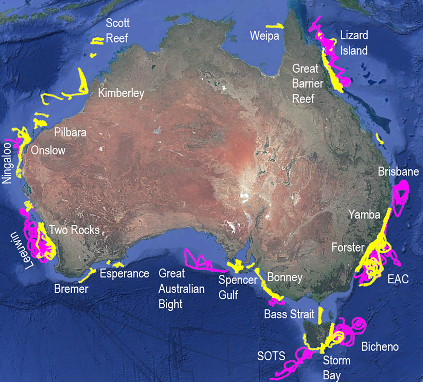
Ocean glider deployments around Australia 2009-2024, representing 9289 glider days (>25 years) and 201,152 km traversed. Seaglider deployments are in purple, Slocum deployments in yellow. Background imagery from Google Earth with sources from Data SIO, NOAA, U.S. Navy, GEBCO and Image Landsat/Copernicus.
Due to the longevity of the IMOS glider program (>16 years) and the very high-resolution nature of the data streams, IMOS holds a huge repository of data. Such long-term datasets open the door to ‘big data’ analyses, where researchers can aggregate missions from the same region across years to understand coastal oceans, their climatology, and the potential impacts of climate change (Malan et al., 2023).
Despite the great value of glider datasets, researchers have voiced concern over the comparability of bio-optical datasets between missions, particularly estimates of Chl (an essential ocean variable; https://gcos.wmo.int/en/essential-climate-variables). The concern is that the bio-optical data has been collected over the years by different sensors on different gliders, and that the potential differences in the calibration of these sensors has never been quantified. IMOS gliders use Sea-Bird Scientific (formerly WET Labs) ECOPuck instruments to measure Chl fluorescence, scatter (a proxy for turbidity) and CDOM fluorescence. Over the years, the ECOPuck models in gliders have been updated and changes in calibration procedures have occurred. There have also been advances in understanding Chl fluorescence, and a global study has quantified the relationship between Chl fluorescence and in situ Chl concentrations (Roesler et al., 2017). Quantifying potential differences within and between IMOS glider sensors and furthering our understanding of the variability of Chl fluorescence, is therefore a timely exercise.
Here we set out to understand potential sources of variability in instrument output. Firstly, to determine the validity of comparing Chl, scatter and CDOM estimates between IMOS missions, we evaluate ECOPuck instrument stability over time by comparing calibration scale factors (SFs) within and between instruments following successive calibrations. We then use laboratory experiments with different phytoplankton groups to determine variability in ECOPuck Chl fluorescent responses. Finally, we evaluate the accuracy of Chl estimates from IMOS gliders by comparing Chl fluorescence from a CTD-mounted glider with in situ extracted Chl concentrations obtained via bottle samples and High Performance Liquid Chromatography (HPLC) analysis.
Methods
IMOS ocean gliders are equipped with Sea-Bird Scientific ECOPucks, a miniaturized version of the Environmental Characterization Optics (ECO) series of instruments that use LED lasers and detectors to measure optical parameters. Teledyne Slocum gliders are fitted with either the FLBBCDSLC and FLBBCDSLK models, which detect Chl fluorescence (470 nm excitation/695 nm emission), CDOM fluorescence (370 nm excitation/460 nm emission) and scatter (700 nm at a scattering angle of 117°). Seagliders were fitted with BBFL2VMT ECOPucks with identical laser excitation and emission spectra for Chl and CDOM, but with scatter detected at 650 nm (except BBFL2VMT #454 and #455 sensors, which detected at 660 nm at a scattering angle of 117 °). The single BBFL2SLO 544 sensor was fitted to a G1 Slocum glider with standard Chl and CDOM fluorescence excitation/emission wavelengths detailed above, but with scatter detected at 650 nm.
Calibrations of glider-based bio-optical instruments are required to relate instrument voltage (counts) to engineering units for fluorescence and scattering via SFs. For Chl fluorescence, factory calibrations are performed using a fluorescein (e.g. uranine) dilution series that is compared against a reference instrument that was originally calibrated using both fluorescein and a monoculture of the diatom species Thalassiosira weissflogii. For CDOM calibration, a quinine sulphate (QSU) standard is used. Scattering is an optical measure of suspended particulate matter concentration and the ECOPuck is configured to measure scattering at 117° using a single LED source and detector. Factory calibration of the scattering sensor is performed using microbeads, yielding scattering data as a volume scattering function (VSF), β(θ,λ), with units of m-1 sr-1, where θ = angle and λ= wavelength. In-water VSF data includes scattering by particles and the seawater itself, but we have improved these data by calculating the particle backscattering coefficient (BBP; m-1) which includes only scattering by particles, as detailed in Mantovanelli and Thomson (2016) and Woo and Gourcuff (2023). Dark counts for each instrument channel are obtained by covering detectors with black tape and submersing the sensor in water. These are base levels of instrument noise and are used in correcting raw instrument counts (Woo and Gourcuff, 2023).
Manufacturer instrument characterization sheets state that “scale factors (SF) for both chlorophyll and CDOM fluorescence are calculated using the equation SF = x ÷ (output – dark counts), where x is the concentration of the solution used during instrument characterization. The SF is used to derive instrument output from the raw signal output of voltage or counts of the fluorometer”. For scattering, the calibration SF is calculated as β(θc)/counts. Chl concentration (µg L-1), CDOM concentration (ppb) and volume scattering function (m-1 sr-1) are computed using SFs and instrument counts, following:
Parameter = SF * (Counts – Dark Counts).
Repeated calibrations over time against reference instruments and solutions therefore provides SFs that can be used to assess changes in instrument performance and inform on stability between calibrations and comparability of instruments over time.
Instrument stability over time
To understand comparability between the same and different instruments over time, we used successive manufacturer calibration SFs for each parameter from 13 different ECOPucks (from both Seaglider and Slocum gliders; Table 1, Supplementary Table 1, Figure 2). This generally included only two successive calibrations, although instruments VMT-454 and VMT-677 had three successive calibrations. From these, we evaluated calibration intervals, SFs, percent change in SFs between calibrations, and the percent maximum SF difference within each instrument model. We noted Customer Alerts where WET Labs changed calibration procedures, and we corrected SFs according to their advice. We illustrate the effect of the change in calibration procedure for Chl fluorescence from July 2011 for all instruments built or characterized before January 2011 by WET Labs (Figure 2) (WET Labs Customer Alert: Chlorophyll-a SFs Shift, July 2011). For scatter, the detection wavelengths varied between sensors, with scatter detected at either 650 nm, 660 nm or 700 nm (Supplementary Table 1). For CDOM, WET Labs advised of a CDOM SF shift for all sensors built or calibrated between January 2008 and August 2010 (CDOM Customer Alert: September, 2010, CDOM SFs Shift). As per WET Labs advice for comparing scaled values, we have adjusted the appropriate SFs by multiplying by 0.63 (asterisks on data in Supplementary Table 1, Supplementary Figures 1a, b). We present dark count ranges but do not further analyze dark counts as they are already incorporated into the supplied SFs.
Table 1
| ECOPuck model | # Sensors | Cal interval (Range) (y) | Dark count range | Scale Factor (SF) range | % change in SF after calibration | Mean SF & max % difference for model |
|---|---|---|---|---|---|---|
| Chl FLU | Chl FLU (µg L-1 count-1) | |||||
| BBFL2SLO | 1 | 3.1 | 47 - 50 | 0.0119 - 0.0123 | 3.4 | – |
| BBFL2VMT | 7 | 1.6 - 5.0 | 45 - 59 | 0.0105 - 0.0138 | -4.0 - 9.0 | 0.0119, 15%* |
| FLBBCDSLK | 3 | 2.4 - 5.3 | 40 - 54 | 0.0072 - 0.0122 | -5.8 - 2.5 | |
| FLBBCDSLC | 2 | 5.8 - 8.8 | 40 - 47 | 0.0072 - 0.0073 | 0 - 1.4 | 0.0073, 1.8%** |
| Scatter | Scatter (x 10-6, m-1 sr-1 count-1) |
|||||
| BBFL2SLO | 1 | 3.1 | 35 - 58 | 3.88 - 6.35 | 63.8 | – |
| BBFL2VMT | 7 | 1.6 - 5.0 | 39 - 59 | 2.98 - 4.06 | -14.3 - 6.7 | 3.6 x 10⁻⁶, 18% |
| FLBBCDSLK | 3 | 2.4 - 5.3 | 41 - 49 | 1.90 - 2.95 | -0.9 – 35.5 | 2.1 x 10⁻⁶, 37% |
| FLBBCDSLC | 2 | 5.8 - 8.8 | 38 - 47 | 1.58 - 2.18 | 4.8 - 38.1 | 2.0 x 10⁻⁶, 18% |
| CDOM | CDOM (ppb count-1) | |||||
| BBFL2SLO | 1 | 3.1 | 66 - 67 | 0.0820 - 0.0931 | 11.5 | – |
| BBFL2VMT | 7 | 1.6 - 5.0 | 36 - 84 | 0.087 - 0.1084 | -6.7 - 28.5 | 0.0944, 17% |
| FLBBCDSLK | 3 | 2.4 - 5.3 | 41 - 46 | 0.0724 - 0.0900 | -0.56 - -19.56 | 0.0864, 16% |
| FLBBCDSLC | 2 | 5.8 - 8.8 | 39 - 48 | 0.0894 - 0.0931 | 1.68 - 3.1 | 0.0909, 2.4% |
Data for WET Labs ECOPuck models and their ranges for calibration intervals, and scale factors (SFs) for chlorophyll fluorescence, scatter and CDOM fluorescence before and after calibration for models BBFL2SLO, BBFL2VMT, FLBBCDSLK and FLBBCDSLC.
*indicates VMT and SLK models with same calibration method were grouped together for calculating the mean value.
**indicates that SLK and SLC models with same calibration method were grouped together for mean value.
Figure 2
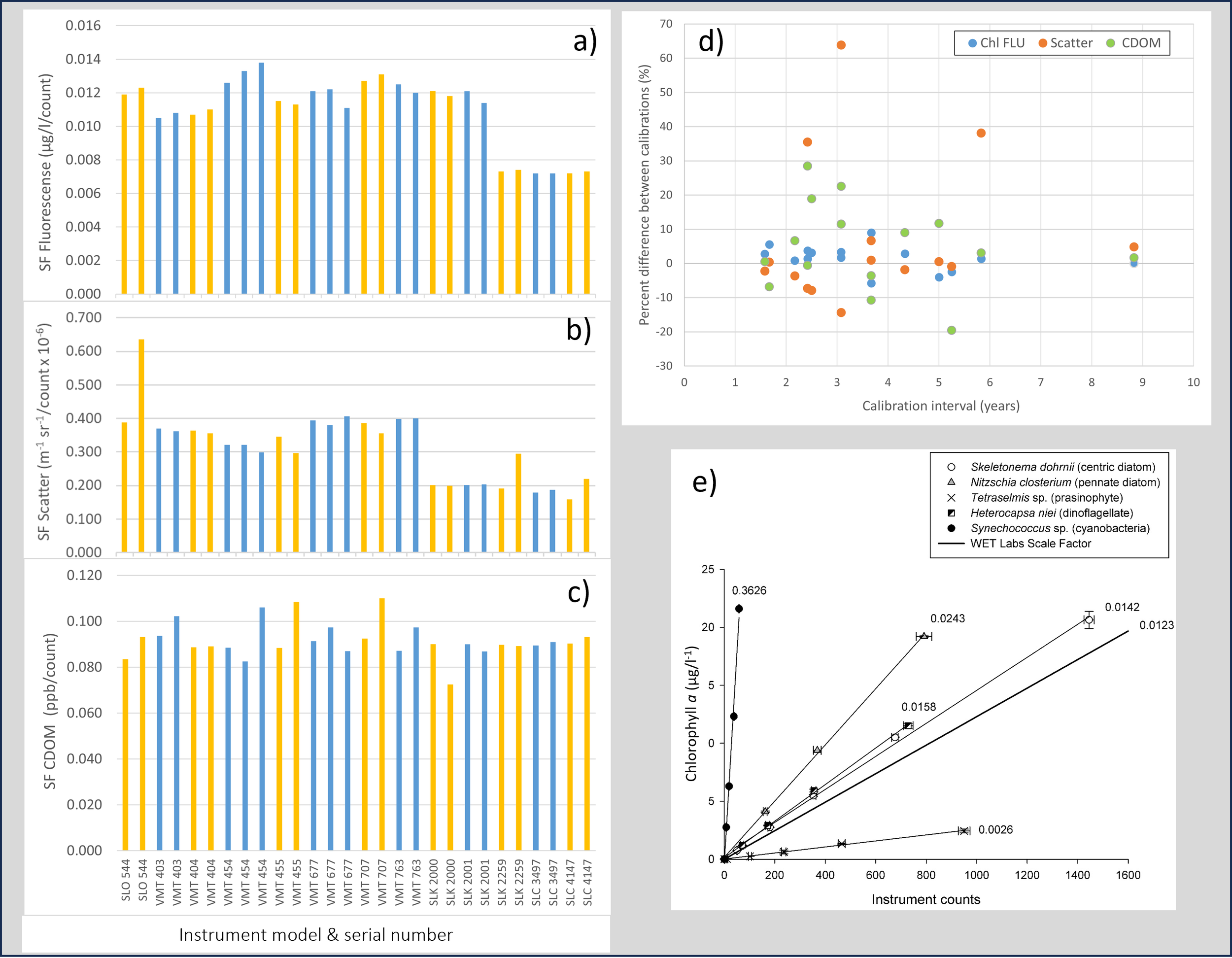
(a-c) WET Labs scale factors (SFs) for chlorophyll fluorescence, scatter and CDOM fluorescence before and after calibration in sequential colored pairs or triplets for ECOPuck models BBFL2SLO, BBFL2VMT, FLBBCDSLK and FLBBCDSLC, (d) percent change in SFs between calibrations plotted against calibration interval, and (e) instrument response (chlorophyll fluorescence counts from ECOTriplet FLBBCDSLK 625) to serial dilutions of individual laboratory cultures of 5 phytoplankton species (extracted chlorophyll a; µg/L), and calculated SFs for each species (numbered per line).
Fluorescent response by different phytoplankton groups
To understand potential biotic sources of variation in instrument output, we used five phytoplankton cultures (Supplementary Table 2) obtained from the Australian National Algae Culture Collection (https://www.csiro.au/en/about/facilities-collections/collections/anacc) to determine their fluorescent response to a Sea-Bird Scientific FLBBCDSLK ECOTriplet (625) instrument and their fluorescence:Chl-a ratios. The ECOTriplet is an autonomous, stand-alone version of the miniaturized ECOPuck with up to three optical sensors. The FLBBCDSLK ECOTriplet has identical detection characteristics to the FLBBCDSLK/SLC miniaturized ECOPucks used in our gliders, being Chl fluorescence (470 nm excitation/695 nm emission), CDOM fluorescence (370/460 nm) and scatter (700 nm at a scattering angle of 117°). The Chl and CDOM excitation bandwidths for the ECOTriplet have been noted as approximately ±10 nm (Earp et al., 2011). Phytoplankton cultures in the exponential growth phase were placed in a dark chamber under ambient temperatures (ca. 18 °C) and low light conditions exterior to the chamber, and their fluorescent response was measured in triplicate over a 5-point dilution series. Up to 500 mL of culture from each dilution step was filtered through Whatmann GF/F filters, followed by Chl-a extraction in 90% acetone using standard procedures (Parsons et al., 1984) and measurement via Turner Designs 10AU fluorometer.
Relationship of chlorophyll fluorescence & in situ chlorophyll concentrations
To understand how well ECOPuck fluorescence can estimate Chl concentrations, we compared ECOPuck measurements with bottle Chl-a samples by attaching a Slocum glider to the CTD carousel on the RV Solander over 2 cruises (Figure 3a) or by sampling waters nearby a diving glider. Waters off Western Australia are typically oligotrophic, with very low chlorophyll surface waters overlaying a deep chlorophyll maximum (Hanson et al., 2007). We identified the chlorophyll maximum on each cast and took seawater samples at this depth for the comparisons. However, to minimize effects of non-photochemical quenching (NPQ) that could confound the comparisons, where possible, we included only samples from depths with a photosynthetically active radiation (PAR) level of ≤ 200 μEin m−2 s−1 (Roesler et al., 2017). Up to 3L of seawater from the bottle samples were filtered through Whatman GF/F filters, which were frozen in liquid nitrogen until HPLC analysis (within 3 months) by the Commonwealth Scientific and Industrial Research Organization (CSIRO). ECOPuck measurements were averaged in 1 m depth bins corresponding to the bottle samples. In 2015, we used 13 paired bottle/ECOPuck samples along the 100 m depth contour of the North West Shelf of Western Australia. In 2016, we used 18 opportunistic paired samples in tropical waters on the continental shelf and over the oceanic Sahul Shoals in the Timor Sea. In 2017, we used 11 paired bottle samples within 24 hrs of the path of a deployed glider at continental shelf sites off WA's Ningaloo Reef. To examine relationships between Chl estimates, we performed point-by-point regression analyses for each year.
Figure 3
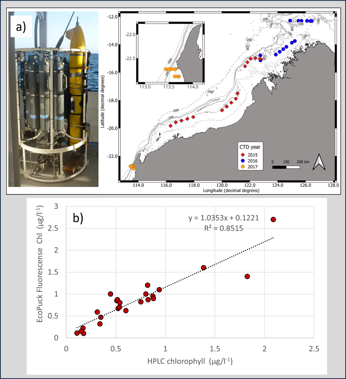
(a) Slocum glider attached to the CTD carousel onboard the RV Solander and CTD sites in 2015 and 2016 on the North West Shelf of Australia, and in 2017 at Ningaloo Reef (inset), and (b) Correlation of glider ECOPuck chlorophyll florescence estimates against HPLC Chl-a estimates from CTD bottle samples taken at same depth in 2015 on the North West Shelf of Australia.
Results
Instrument stability over time
Calibration data for each sensor are summarized in Table 1, with full analytical details provided in Supplementary Table 1. Initial calibration data from older sensors reaches back to 2008 (BBFL2SLO and BBFL2VMT), with the latest data from 2021. Intervals between factory calibrations ranged between 1.6–5 yrs, although intervals for FLBBCDSLK-2000, FLBBCDSLC-3497 and FLBBCDSLC-4147 were longer at 5.3, 8.8 and 5.8 yrs, respectively (Table 1, Supplementary Table 1). Dark counts could be variable within an instrument model (Table 1), but we found no relationships between changes in dark counts and calibration intervals, or between instruments (data not shown); dark counts are therefore not considered further.
Chl SFs were highest in the BBFL2SLO and BBFL2VMT sensors and lower in the FLBBCDSLK and FLBBCDSLC sensors, reflecting the change in calibration procedures instigated by WET Labs in 2011 to reduce instrument to instrument variability (Figure 2a). Between calibrations, Chl SFs for individual sensors for all models were stable, changing by <10% (Table 1, Figures 2a, d, Supplementary Table 1). Of this small variability, the greatest change of 9% occurred in BBFL2VMT 677 (Supplementary Table 1). Otherwise, maximum differences following calibration for the BBFL2SLO, FLBBCDSLK and FLBBCDSLC sensors were 3.4%, -5.8% and 1.4%, respectively. In terms of comparability between sensors of the same model, SFs showed generally limited variability around a calculated mean value (Table 1, Figure 2a). For Chl, most percent differences were ≤ 9% (although where the BBFL2VMT and FLBBCDSLK shared the older calibration method and thus similar SFs, the maximum difference from the mean SF of 0.0119 was 15%). For the grouped FLBBCDSLK and FLBBCDSLC models that shared the later calibration method, the maximum difference from the mean SF of 0.0073 was only 1.8% (Table 1).
Scale factors for scatter across all sensors showed a similar pattern to those for Chl fluorescence, being higher in the BBFL2SLO and BBFL2VMT models and lower in the FLBBCDSLK and FLBBCDSLC sensors (Table 1, Figure 2b). Rather than reflecting a change in calibration procedure, this difference appears due to sensors being fitted with different detector wavelengths, with the BBFL2VMT models detecting scatter at either 650 or 660 nm while the FLBBCDSLC and FLBBCDSLK sensors used 700 nm. Following calibration, scatter SFs were similarly stable like those for Chl. Amongst the BBFL2VMT sensors, SF change after calibration ranged between -14.3% – 6.7%, with only 1 sensor (#455) exceeding >10% change (Supplementary Table 1). Scale factors amongst the FLBBCDSLK and FLBBCDSLC sensors were generally very similar with changes of <5% (except for sensors #2259 and #4147 with 35.5% and 38%, respectively; Figure 2a, Table 1, Supplementary Table 1). The SF for BBFL2SLO-544 increased by 63% after the initial calibration, a large change not reflected in Chl or CDOM fluorescence. Percent differences between the same instrument models were larger than that found for Chl, although differences in detection wavelength confounds this descriptor somewhat. The maximum variation from the mean SF for the BBFL2VMT and FLBBCDSLC sensors was 17%, while it reached 37% in the FLBBCDSLK model (Table 1).
Scale factors for CDOM are presented here following correction advice from the WET Labs Customer Alert, and the uncorrected SFs are plotted in Supplementary Figures 1a, b. Overall, CDOM SFs ranged between 0.0724–0.1084 x 10⁻⁶ m-1 sr-1 count-1 (Figure 2c, Table 1). Even post-correction, CDOM SFs were variable: five of the seven BBFL2VMT sensors had SFs exceeding 10% change (reaching a maximum of 28.5%), while one of the three FLBBCDSLK sensor SFs decreased by -19.6% between calibrations. Otherwise, SFs for CDOM following calibration in the remaining FLBBCDSLK and FLBBCDSLC sensors varied by ≤ 3.1%. The SF for BBFL2SLO 544 was relatively stable between calibrations, increasing by 11.5% (Supplementary Table 1). Scale factors within the models varied from the mean by maximums of 17%, 16% and 2.4% for BBFL2VMT, FLBBCDSLK and FLBBCDSLC, respectively (Table 1).
Based on the sensors BBFL2VMT-454 and -677 with three successive calibrations, we did not see a pattern of SF increase or decrease for any variable (Figure 2). The Chl SF for #454 increased marginally with each calibration, while the SF for #677 initially remained stable but then decreased following the third calibration. Scatter SFs remained similar, while CDOM SFs variably increased or decreased slightly between calibrations (Supplementary Table 1). Overall, combining data from all sensors and parameters, there appeared to be no relationship between calibration interval and SF changes (Figure 2d). For example, the longest Chl calibration intervals of 5.8 and 8.8 yrs occurred in the FLBBCDSLC sensors where changes in SF was very low (0–1.4%). This contrasted with higher percent changes in the older sensors where calibration intervals were shorter (1.6 – 5.3 yrs). This lack of relationship was also reflected in the scatter and CDOM SFs (Figure 2d).
Fluorescent response by different phytoplankton groups
All phytoplankton species displayed various linear relationships between instrument counts (Chl fluorescence) and extracted Chl-a (Figure 2e), illustrating the underlying complexity of using fluorescence as a proxy for Chl concentration. The centric diatom species Skeletonema dohrnii had a SF of 0.0142, and was the most similar to the WET Labs-supplied SF of 0.0123 for the instrument; this seems reasonable considering the latter was determined using a monoculture of the diatom Thalassiosira weissflogii. The dinoflagellate Heterocapsa niei also had a similar SF (0.0158), although the pennate diatom Nitzschia closterium (common in WA waters) had a SF approximately twice that of the WET Labs SF. Synechococcus sp. and Tetraselmis sp. showed a much poorer linear relationship compared to the diatoms and the dinoflagellate. The SF for Synechococcus sp. of 0.3626 was much higher than that of the instrument, indicative of a species that exhibits low fluorescence even at high Chl concentrations. Conversely, the SF for Tetraselmis sp. of 0.0026 was much lower than that of the instrument, indicating a species that exhibits high florescence even at low Chl concentrations.
Relationship of chlorophyll fluorescence & in situ chlorophyll concentrations
In situ HPLC-analyzed Chl-a concentrations during the 2015, 2016 and 2017 cruises reached 2.1 µg l-1, but were generally exceeded by ECOPuck estimates which reached 2.7 µg l-1. Despite this, we found positive relationships between ECOPuck and in situ HPLC Chl estimates from each cruise. In 2015, the ECOPuck Chl estimates were a good predictor of in situ HPLC-measured values (R2 = 0.82; Figure 3b), although relationships were somewhat poorer in 2017 (R2 = 0.68; Supplementary Figure 2), and poorest in 2016 (R2 = 0.60; Supplementary Figure 3). In each year, ECOPuck estimates were generally higher than those by HPLC, with mean ECOPuck: HPLC Chl-a ratios of 1.2:1, 2.9:1 and 1.1:1 in 2015, 2016 and 2017, respectively (Supplementary Figures 2–4).
Discussion
Our major question was whether estimates of bio-optical parameters (Chl, scatter and CDOM) are comparable over the long term at repeat IMOS glider sites, given that different ECOPuck sensors of the same or similar models are used on different gliders. For the essential ocean variable Chl, the answer is yes, given the stability of SFs following successive calibrations and within the different instrument models demonstrated here. For scatter and CDOM, the answer is a more cautious and qualified yes, as the higher inherent variability in these parameters (and an understanding of it) may be acceptable in some studies. However, the responses of phytoplankton species to the ECOPuck are a clear source of variability in Chl fluorescence estimates that are difficult to quantify, and we have illustrated this variability. Finally, our comparisons between bottle Chl-a samples by HPLC and ECOPuck Chl estimates during ocean sampling on three cruises showed that the ECOPuck can overestimate Chl by up to 2.9 times the actual concentration (consistent with the analyses of Roesler et al., 2017). Thus, while the instruments may be stable over time, other factors have greater influence on the variably and comparability of ECOPuck Chl estimates.
We found that SFs for Chl fluorescence were stable for individual sensors following successive calibrations (maximum change of <9%), and also comparable within sensor models (maximum difference of 15%). This low SF variability means that the different sensors of the same model are highly comparable across different missions and over time. The SLK and SLC sensors in the IMOS Slocum fleet were particularly stable, and although only 5 sensors were used in this study, this stability reflects well on the other 14 sensors of these models that have been, or are now, deployed within our fleet. This finding is significant as it enhances the usefulness and application of this essential ocean variable data stream to different research questions from long-term IMOS glider mission sites around Australia (Bahmanpour et al., 2016; Lauton et al., 2021; Chen et al., 2020; Mahjabin et al., 2020; Schaeffer et al., 2016).
We observed differences in Chl fluorescence SFs from ECOPucks in the Slocum gliders and those fitted to Seagliders due to a change in the factory calibration procedure. For IMOS operations, this is not necessarily an issue as our Slocum gliders operate on the continental shelf to 200 m depth, while the Seagliders operated in deeper waters off the shelf. However, depending on the research question, it may be advisable to use ratios of mean SFs to combine Slocum and Seaglider Chl estimates across shelf regions (a strategy suggested by WET Labs to correct SFs between calibration changes).
Scatter and CDOM SFs were generally more difficult to assess due to changes in detection wavelength and calibration procedures. However, it appears that scatter and CDOM data may be less comparable over the long term with different instruments due to SF variability. Most sensors had scatter SFs that changed little following calibrations (<8%); however, if the notably variable SLK instrument was removed from the calculation, the within-model variation was 11.3–18% from the mean SF. The within-model SF variation for CDOM was similarly high (17%), although the within-SLC instrument variability was low and shows promise for stability in the future with this more recent model. Whether or not this higher within-instrument variability is acceptable for different studies is a question for specific researchers (who must also consider the potential impact of CDOM on Chl signals; Breves et al., 2003; Coble, 2007). However, it does not diminish the usefulness of these data streams for understanding the effects of some ocean processes (e.g. Baird et al., 2011; Pattiaratchi and de Oliveira, 2016; Malan et al., 2024).
Due to logistical and operational considerations, the time between calibrations for IMOS glider instruments exceed the recommended 1-year interval recommended by Teledyne. Australia is relatively remote from USA- and UK-based service centers; sending instruments to the USA for calibration results in turn-around times of at least 3 months, and in the case of some instruments, much longer. Thus, keeping to an annual calibration schedule for instruments with these return times is impracticable. Instead, IMOS Ocean Gliders strives to return instruments for calibration after one year of in-water use. With average glider deployment durations of 21 days, even a heavily-used glider would require instrument calibration less frequently than one calendar year. This policy has also limited the number of sensors with multiple, repeat calibrations, a situation exacerbated by the loss of gliders (and instruments) at sea and by retirement of the Seaglider fleet from our operations.
A larger potential source of variation than the instrument itself is the fluorescent response of different phytoplankton species. Scale factors from factory calibrations are based on a quantified transfer function between the calibration fluid and the initial response of a culture of the centric diatom Thalassiosira weisflogii over a dilution series. However, we found that the response of other species varied widely from the centric diatom, with that of the prasinophyte Tetraselmis sp. and the cyanobacteria Synechococcus sp. drastically over- and under-estimating Chl concentrations, respectively. Variability in the fluorescent response of phytoplankton species has been observed in other studies and is attributed to different reasons (Roesler et al., 2017; Proctor and Roesler, 2010). In particular, the 470 nm excitation wavelength of the ECOPuck targets photosynthetic accessory pigments, rather than Chl-a, thus the pigment content of different phytoplankton species will influence the fluorescent response and subsequent chlorophyll estimates. Furthermore, other biotic and abiotic factors such as lifecycle stage, time of day, nutrient availability and depth are all known to affect phytoplankton fluorescence (Abbott et al., 1982; Proctor and Roesler, 2010). Overall, phytoplankton community composition and other environmental factors will all play a role in Chl estimates from ECOPuck fluorescence. Specific methods to correct for non-photochemical quenching in shelf-based ocean glider datasets are becoming available (e.g. Mitchell et al., 2024), and will be an important consideration for furthering IMOS Ocean Gliders QA/QC Best Practice (Woo and Gourcuff, 2023).
Finally, from our in situ paired-sample studies between ECOPuck and HPLC-analyzed bottle samples, we found that ECOPucks overestimated Chl by mean values of 1.1–2.9 times. Our best match ups occurred in 2015 and 2017 where samples were taken consistently in similar environments, either along the 100 m depth contour of WA’s North West Shelf, or across the shelf of Ningaloo Reef. Our highest overestimate of 2.9:1 occurred from the variable depth environment of the oceanic shoals and a shelf break, taken also during a marine heatwave (Le Nohaïc et al., 2017). It seems likely that differing phytoplankton communities from different environments confound the comparisons somewhat, producing the overestimations that we recorded. Our findings are similar to those from a global WET Labs ECO instruments study, where the mean ratio of fluorescence:HPLC-analysed Chl-a values was 2:1 (Roesler et al., 2017). Glider missions are highly likely to sample a wide range of different environments within a single mission, so would likely experience similar effects. Like the ARGO float program, one option is to take paired samples for HPLC Chl-a analyses at the start of the glider deployment to calibrate the ECOPuck values (Schmechtig et al., 2015). However, while these calibrations are valid for the specific deployment location and time, our data indicates that their validity may be affected by differing phytoplankton community composition encountered by the glider in different locations.
In summary, we found that SFs for chlorophyll fluorescence following successive factory calibrations of the ECOPucks were stable, and that these SFs varied minimally between instruments of the same models. This finding is significant as it demonstrates the comparability of Chl data between missions, which is crucial for long-term studies of our changing oceans. Scale factors for scatter and CDOM were less stable but not unusably so, and these data may be suitable for combining over multiple missions depending on the specific research questions being addressed. Causes for greater variability and inaccuracies in the Chl output, however, are both biotic and abiotic. Like other studies, we found that the fluorescent response of different phytoplankton species varied greatly from that of the centric diatom monoculture upon which the factory SF was initially based. Furthermore, our in-water match ups between ECOPuck and HPLC-analyzed Chl-a indicated that the instrument overestimated Chl by 1.1–2.9 times, a finding that is comparable to a global study of ECO-series instruments.
Statements
Data availability statement
The original contributions presented in the study are included in the article/Supplementary Material. Further inquiries can be directed to the corresponding author.
Author contributions
PT: Conceptualization, Data curation, Formal Analysis, Investigation, Methodology, Validation, Visualization, Writing – original draft. CP: Funding acquisition, Methodology, Project administration, Resources, Supervision, Writing – review & editing. CH: Formal Analysis, Investigation, Methodology, Validation, Visualization, Writing – review & editing.
Funding
The author(s) declared that financial support was received for this work and/or its publication. Data were sourced from Australia’s Integrated Marine Observing System (IMOS) – IMOS is enabled by the National Collaborative Research Infrastructure Strategy (NCRIS). It is operated by a consortium of institutions as an unincorporated joint venture, with the University of Tasmania as Lead Agent.
Acknowledgments
Data were sourced from Australia’s Integrated Marine Observing System (IMOS) – IMOS is enabled by the National Collaborative Research Infrastructure Strategy (NCRIS). It is operated by a consortium of institutions as an unincorporated joint venture, with the University of Tasmania as Lead Agent.
Conflict of interest
The author(s) declared that this work was conducted in the absence of any commercial or financial relationships that could be construed as a potential conflict of interest.
The author CP declared that they were an editorial board member of Frontiers, at the time of submission. This had no impact on the peer review process and the final decision.
Generative AI statement
The author(s) declared that generative AI was not used in the creation of this manuscript.
Any alternative text (alt text) provided alongside figures in this article has been generated by Frontiers with the support of artificial intelligence and reasonable efforts have been made to ensure accuracy, including review by the authors wherever possible. If you identify any issues, please contact us.
Publisher’s note
All claims expressed in this article are solely those of the authors and do not necessarily represent those of their affiliated organizations, or those of the publisher, the editors and the reviewers. Any product that may be evaluated in this article, or claim that may be made by its manufacturer, is not guaranteed or endorsed by the publisher.
Supplementary material
The Supplementary Material for this article can be found online at: https://www.frontiersin.org/articles/10.3389/fmars.2026.1703896/full#supplementary-material
References
1
Abbott M. R. Richerson P. J. Powell T. M. (1982). In situ response of phytoplankton fluorescence to rapid variations in light. Limnol. Oceanogr.27, 218–225. doi: 10.4319/lo.1982.27.2.0218
2
Bahmanpour M. H. Pattiaratchi C. Wijeratne E. M. S. Steinberg C. D'Adamo N. (2016). Multi-year observation of Holloway Current along the shelf edge of north western Australia. J. Coast. Res.75, 517–521. doi: 10.2112/SI75104.1
3
Baird M. E. Suthers I. M. Griffin D. A. Hollings B. Pattiaratchi C. Everett J. D. et al . (2011). The effect of surface flooding on the physical–biogeochemical dynamics of a warm-core eddy off southeast Australia. Deep. Sea. Res. Part II.: Top. Stud. Oceanogr.58, 592–605. doi: 10.1016/j.dsr2.2010.10.002
4
Breves W. Heuermann R. Reuter R. (2003). Enhanced red fluorescence emission in the oxygen minimum zone of the Arabian Sea. Ocean. Dyn.53, 86–97. doi: 10.1007/s10236-003-0026-y
5
Chen M. Pattiaratchi C. B. Ghadouani A. Hanson C. (2020). Influence of storm events on chlorophyll distribution along the oligotrophic continental shelf off south-western Australia. Front. Mar. Sci.7, 287. doi: 10.3389/fmars.2020.00287
6
Coble P. G. (2007). Marine optical biogeochemistry: the chemistry of ocean color. Chem. Rev.107, 402–418. doi: 10.1021/cr050350+
7
Earp A. Hanson C. E. Ralph P. J. Brando V. E. Allen S. Baird M. et al . (2011). Review of fluorescent standards for calibration of in situ fluorometers: Recommendations applied in coastal and ocean observing programs. Opt. Expr.19, 26768–26782. doi: 10.1364/OE.19.026768
8
Glenn S. M. Miles T. N. Seroka G. N. Xu Y. Forney R. K. Yu F. et al . (2016). Stratified coastal ocean interactions with tropical cyclones. Nat. Commun.7, 10887. doi: 10.1038/ncomms10887
9
Hanson C. E. Pesant S. Waite A. M. Pattiaratchi C. B. (2007). Assessing the magnitude and significance of deep chlorophyll maxima of the coastal eastern Indian Ocean. Deep-Sea. Res. II.54, 884–901. doi: 10.1016/j.dsr2.2006.08.021
10
Hanson C. E. Woo L. M. Thomson P. G. Pattiaratchi C. B. (2016). Observing the ocean with gliders: Techniques for data visualization and analysis. Oceanography30, 222–227.
11
Holbrook N. J. Sen Gupta A. Oliver E. C. J. Hobday A. J. Benthuysen J. A. Scannell H. A. et al . (2020). Keeping pace with marine heatwaves. Nat. Rev. Earth Environ.1, 482–493. doi: 10.1038/s43017-020-0068-4
12
Lauton G. Pattiaratchi C. B. Lentini C. A. D. (2021). Observations of breaking internal tides on the Australian North West Shelf Edge. Front. Mar. Sci.8, 629372. doi: 10.3389/fmars.2021.629372
13
Le Nohaïc M. Ross C. L. Cornwall C. E. Comeau S. Lowe R. McCulloch M. T. et al . (2017). Marine heatwave causes unprecedented regional mass bleaching of thermally resistant corals in northwestern Australia. Sci. Rep.7, 14999. doi: 10.1038/s41598-017-14794-y
14
Liblik T. Karstensen J. Testor P. Alenius P. Hayes D. Ruiz S. et al . (2016). Potential for an underwater glider component as part of the Global Ocean Observing System. Methods Oceanogr.17, 50–82. doi: 10.1016/j.mio.2016.05.001
15
Mahjabin T. Pattiaratchi C. Hetzel Y. (2020). Occurrence and seasonal variability of dense shelf water cascades along Australian continental shelves. Sci. Rep.10, 9732. doi: 10.1038/s41598-020-66711-5
16
Malan N. Roughan M. Hemming M. Ingleton T. (2024). Quantifying coastal freshwater extremes during unprecedented rainfall using long timeseries multi-platform salinity observations. Nat. Commun.15, 424. doi: 10.1038/s41467-023-44398-2
17
Malan N. Roughan M. Hemming M. Schaeffer A. (2023). Mesoscale circulation controls chlorophyll concentrations in the East Australian Current separation zone. J. Geophys. Res.: Ocean.128, e2022JC019361.
18
Mantovanelli A. Thomson P. (2016). “ Particle backscattering coefficient,” in Integrated marine observing system. (Perth, Western Australia: IMOS Ocean Gliders). Available online at: https://content.aodn.org.au/Documents/IMOS/Facilities/Ocean_glider/Backscatter_correction.pdf (Accessed April 2016).
19
Mitchell C. Drapeau D. Pinkham S. Balch W. M. (2024). A chlorophyll a, non-photochemical fluorescence quenching correction method for autonomous underwater vehicles in shelf sea environments. Limnol. Oceanogr. Methods22, 149–158. doi: 10.1002/lom3.10597
20
Parsons T. R. Maita Y. Lalli C. M. (1984). A manual of chemical and biological methods for seawater analysis (Oxford: Pergamon Press).
21
Pattiaratchi C. de Oliveira G. L. (2016). “ Sediment re-suspension processes along the Australian north-west shelf revealed by ocean gliders,” in 20th australasian fluid mechanics conference (Perth, Western Australia, Australia: Australasian Fluid Mechanics Society).
22
Pattiaratchi C. Woo L. M. Thomson P. G. Hong K. K. Stanley D. (2017). Ocean glider observations around Australia. Oceanography30, 90–91. doi: 10.5670/oceanog.2017.226
23
Proctor C. W. Roesler C. S. (2010). New insights on obtaining phytoplankton concentration and composition from in situ multispectral chlorophyll fluorescence. Limnol. Oceanogr.: Methods8, 695–708. doi: 10.4319/lom.2010.8.695
24
Roesler C. Uitz J. Claustre H. Boss E. Xing X. Organelli E. et al . (2017). Recommendations for obtaining unbiased chlorophyll estimates from in situ chlorophyll fluorometers: A global analysis of WET Labs ECO sensors. Limnol. Oceanogr.: Methods15, 572–585. doi: 10.1002/lom3.10185
25
Schaeffer A. Roughan M. (2015). Influence of a western boundary current on shelf dynamics and upwelling from repeat glider deployments. Geophys. Res. Lett.42, 121–128. doi: 10.1002/2014GL062260
26
Schaeffer A. Roughan M. Austin T. Everett J. D. Griffin D. Hollings B. et al . (2016). Mean hydrography on the continental shelf from 26 repeat glider deployments along Southeastern Australia. Sci. Data3, 160070.
27
Schmechtig C. Poteau A. Claustre H. D’Ortenzio F. Boos E. (2015). “ Processing Bio-Argo chlorophyll-a concentration at the DAC level,” in IFREMER for argo data management.
28
Woo L. M. Gourcuff C. (2023). Delayed mode QA/QC best practice manual version 3.1 integrated marine observing system. (Perth, Western Australia: IMOS Ocean Gliders). doi: 10.26198/5c997b5fdc9bd
Summary
Keywords
chlorophyll-A (CHL), colored dissolved organic matter (CDOM) fluorescence, ocean glider, optical sensor, backscatter
Citation
Thomson PG, Pattiaratchi CB and Hanson CE (2026) Understanding the stability of the ECOPuck optical sensor: evaluation of long-term ocean glider data streams across decades. Front. Mar. Sci. 13:1703896. doi: 10.3389/fmars.2026.1703896
Received
12 September 2025
Revised
05 January 2026
Accepted
06 January 2026
Published
03 February 2026
Volume
13 - 2026
Edited by
Emanuele Organelli, National Research Council (CNR), Italy
Reviewed by
Viviana Piermattei, Foundation Euro-Mediterranean Center on Climate Change (CMCC), Italy
Emmanuel Boss, University of Maine, United States
Updates
Copyright
© 2026 Thomson, Pattiaratchi and Hanson.
This is an open-access article distributed under the terms of the Creative Commons Attribution License (CC BY). The use, distribution or reproduction in other forums is permitted, provided the original author(s) and the copyright owner(s) are credited and that the original publication in this journal is cited, in accordance with accepted academic practice. No use, distribution or reproduction is permitted which does not comply with these terms.
*Correspondence: Christine E. Hanson, christine.hanson@uwa.edu.au
Disclaimer
All claims expressed in this article are solely those of the authors and do not necessarily represent those of their affiliated organizations, or those of the publisher, the editors and the reviewers. Any product that may be evaluated in this article or claim that may be made by its manufacturer is not guaranteed or endorsed by the publisher.