Abstract
Introduction:
High-precision radio wave propagation over maritime environments is of great importance for ensuring reliable maritime wireless communications.
Methods:
To support the development of maritime transmission services, this work employs genetic algorithms to extract features from measured maritime data, thereby constructing a data-model-driven propagation model. The proposed model is established using measurement datasets collected in the South China Sea, covering the frequency range of 99 MHz to 1000 MHz over transmission distances up to 60 km. By integrating the strengths of both data-driven and model-driven approaches, a high-precision empirical model for maritime VHF and UHF propagation loss is developed. Specifically, we first analyze the propagation mechanisms of radio waves in the study region based on the measured data, and then combine them with the ITU-R P.2001 model to define a driving model with undetermined coefficients. These coefficients are subsequently determined using genetic algorithms through feature extraction from the measurement data. Finally, the proposed model is validated against the measurement dataset.
Results:
Results demonstrate that the model achieves an average root-mean-square error of 2.13 dB, representing a 72.73% improvement compared with the ITU-R P.2001 model.
Discussion:
The study of high-precision radio wave propagation over maritime environments is of great importance for ensuring reliable maritime wireless communications.
1 Introduction
Accurate prediction of radio wave propagation characteristics in such environments is crucial for the advancement of future communication systems (Hu et al., 2024; Xu et al., 2023). The vision of sixth-generation (6G) mobile communication is to establish an integrated space–air–ground–sea network (Wang et al., 2021). As an indispensable component of 6G, maritime communications play a pivotal role in extending the global coverage of wireless networks (Xu et al., 2023). Consequently, the design of reliable communication systems and technological innovations in maritime communications have attracted growing research interest (He et al., 2022). The wireless channel provides the propagation medium for radio waves, and understanding its characteristics—shaped by the unique properties of the ocean environment—is essential for optimizing and enhancing maritime communication systems (Wang et al., 2023b). Unlike terrestrial channels, which have been extensively studied, maritime channel analysis and modeling remain relatively underexplored. Therefore, there is an urgent demand for the development of practical and accurate maritime channel models.
Traditional path loss models can generally be classified into three categories according to their modeling approaches: deterministic models, empirical models, and semi-empirical models (Erunkulu et al., 2023). Deterministic models mainly rely on modified ray-tracing (RT) techniques or finite-difference time-domain (FDTD) methods to accurately characterize maritime radio wave propagation. Empirical models, in contrast, are constructed from measured data using statistical fitting approaches (Erunkulu et al., 2023). Semi-empirical models integrate both deterministic and empirical approaches to achieve more precise channel characterization. In recent years, with the rapid advancement of artificial intelligence, intelligent algorithms have introduced a new data-driven paradigm for path loss modeling, leveraging their strong nonlinear modeling capabilities (Seretis and Sarris, 2021). For example, Wang et al. proposed a high-precision FM broadcasting path loss model for the Beijing region by employing measured data as input and applying a long short-term memory (LSTM) neural network algorithm (Wang et al., 2024b). Similarly, Huang et al. developed a radio wave propagation model for tunnel environments based on convolutional neural networks (CNNs) (Huang et al., 2024). Afape et al. proposed a stacking-ensemble regression machine learning model, demonstrating how machine learning techniques can significantly improve prediction accuracy (Afape et al., 2024). To efficiently extract environmental features from satellite imagery, residual structures, attention mechanisms, and spatial pyramid pooling layers have been incorporated into deep neural networks based on domain expertise. For instance, Wang et al. introduced a novel deep learning-based path loss prediction model utilizing satellite images, with validation results showing that the proposed model reduced the root mean square error (RMSE) by 3.07 dB compared with empirical models (Wang et al., 2024a). Although data-driven models based on intelligent algorithms can achieve high prediction accuracy, their generalization capability across diverse environments remains limited (Yang et al., 2023b). The ITU-R P.2001 model, proposed by the International Telecommunication Union, is a widely used universal path loss model (International Telecommunication Union (ITU-R), 2023). Its advantage lies in its broad applicability across different scenarios. However, validation efforts in multiple regions—including Denver, USA (Wang et al., 2023a), Beijing, China (Wang et al., 2024c), and Guizhou, China (Wu et al., 2024)—have shown that the RMSE between predicted and measured values often exceeds 6 dB, failing to meet internationally recognized accuracy requirements (Yang et al., 2023a). Therefore, building upon the ITU-R P.2001 model, the effective integration of intelligent algorithms for feature extraction from measured data to construct a high-precision path loss model is of great significance for supporting maritime wireless transmission services.
To establish a high-precision maritime path loss model, this study proposes a modeling approach based on a hybrid data-model-driven framework. The hybrid data-model-driven approach refers to integrating data-driven modeling and model-driven modeling methods (Zhang et al., 2023). Models driven by data offer higher accuracy, while models driven by models provide better adaptability and stability. By integrating the two approaches, it is possible to combine their respective advantages and develop a more robust and high-performance path loss model. Based on the above modeling approach, the main contributions of this study are as follows: (1) A parameterized model with undetermined coefficients was developed based on the ITU-R P.2001 model. (2) A high-precision empirical maritime path loss model is built by integrating data-driven and model-driven methods.
The structure of this study is organized as follows. Section II introduces the proposed modeling framework, beginning with an overview of the modeling process and describing the measured data used for model development. Based on these data, the propagation mechanisms of radio waves in the study area are analyzed, and a parameterized model with undetermined coefficients is constructed. A Genetic Algorithm (GA) is then employed to optimize these coefficients using maritime measurement data as the data-driven basis, deriving the optimal parameters and establishing a high-precision maritime path loss model. Section III presents a comparative analysis between the ITU-R P.2001 model and the proposed model to evaluate the latter’s performance. Finally, Section IV provides concluding remarks and a summary of the main contributions of this work.
2 Materials and methods
2.1 Modeling approach
Currently, maritime communication systems—such as Vessel Traffic Services (VTS)—primarily rely on Very High Frequency (VHF, 30 MHz–300 MHz) bands for communication (Lee et al., 2017). The World Radiocommunication Conference (WRC) has allocated the 600 MHz–1000 MHz band as a low-frequency range for 5G enhanced Mobile Broadband (eMBB) services (Zhang et al., 2024), which also constitutes a key part of the sub-6 GHz band (450 MHz–1000 MHz) (You et al., 2021). 5G communication is not only an incremental leap in wireless technology but also a potential catalyst for the digital revolution (Majid et al., 2024; Mezaal et al., 2024). To support the development of the current and future maritime wireless transmission services, this study collects data from five key frequencies for modeling research: 99 MHz and 160 MHz in the VHF range, and 600 MHz, 830 MHz, and 1000 MHz in the UHF range.
The modeling process is shown in Figure 1. First, we collected the maritime measurement data used for modeling, including the transmitter and receiver locations, antenna heights, gains, and elevation maps of the modeling area. Next, we analyzed the propagation mechanism of radio waves in the modeling area based on the measured data. On this basis, a parameterized model with undetermined coefficients was constructed, incorporating the ITU-R P.2001 model. Then, we preliminarily estimated the range of the undetermined coefficients in the proposed model based on the maritime measurement data, which was used to define the search space for chromosome optimization in the GA. Subsequently, the GA was initialized, and the undetermined coefficients in the model were optimized based on the test data, resulting in the construction of a high-accuracy maritime path loss model. Finally, we validated the performance of the proposed model. In the following sections, we provide a detailed introduction to each step of the modeling process based on the workflow outlined above.
Figure 1
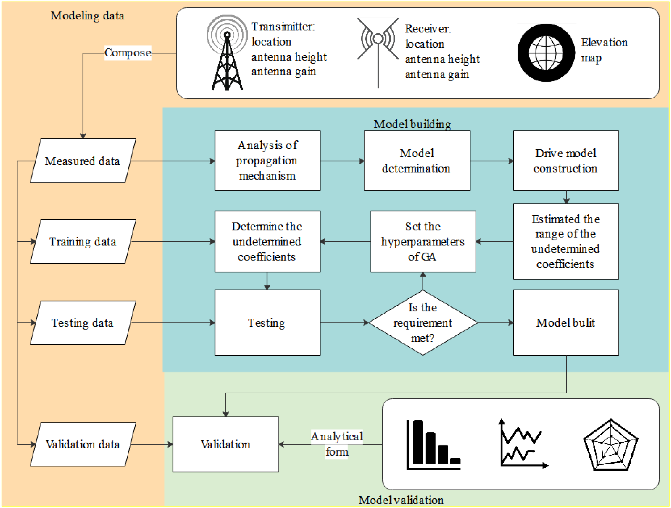
Modeling approach.
2.2 Modeling data
The measurement campaign was conducted in July 2016 under calm sea conditions, surrounding the waters of Hainan Island, South China Sea, with clear weather and no wind, and measurements were carried out during daytime. Under such environmental conditions, the sea surface was relatively smooth, and atmospheric conditions were stable, which helped to reduce additional variability caused by sea clutter, surface roughness, and weather-induced fluctuations. As a result, the measured propagation characteristics are mainly dominated by large-scale path loss mechanisms rather than short-term environmental disturbances. The transmitting antenna was fixed at (18.25°N, 109.42°E) with a mounting height of 24.9 meters, and an azimuth angle of 210°. The model of the signal source is R&S SML03. An R&S HL116 antenna was used for transmission at 99 and 160 MHz, featuring a gain of 0.9 dBi. An R&S HL223 antenna was used for transmission at 600, 830, and 1000 MHz, featuring a gain of 0.9 dBi. The antenna was installed in an open area without any obstructions nearby. An R&S 023A1 antenna was used for the receiving antenna. It was mounted on a research vessel at an elevation of 10.9 meters above sea level. The spectrum analyzer adopts CeyearAV 4036. The vessel sailed southwestward along a 210° azimuth, with its route terminating at (17.84°N, 109.17°E). The total sailing distance was approximately 60 km. Along the route, we evenly deployed 25 data collection points. The gain of the receiving antennas was 6.59 dBi for all frequencies. During the data collection process, the mean detection method was used, with sampling conducted at a rate of once per second. At each observation point, the vessel was anchored, and the spectrum analyzer was configured with a sampling interval of less than 100 ms. The measurement duration at every observation point exceeded 5 minutes. For each frequency, at least 1,000 data samples were collected, resulting in a total of approximately 125,000 data points. The median value of all recorded field strength measurements at each receiving point was adopted as the final result to ensure robustness against outliers. Subsequently, the field strength values were converted to path loss using the methodology outlined in ITU-R P.525 (International Telecommunication Union (ITU-R), 2019). In total, 125 measured samples across five frequencies were utilized for model construction. The detail of the propagation path is shown in Table 1.
Table 1
| Parameter\ Frequency |
99MHz | 160MHz | 600MHz | 830MHz | 1000MHz |
|---|---|---|---|---|---|
| Signal source | R&S SML03 | ||||
| Transmitting antenna | R&S HL116 | R&S HL223 | |||
| Transmitting antenna height | 24.9m | ||||
| Transmitting antenna gain | 0.9 dBi | ||||
| Spectrum analyzer | CeyearAV 4036. | ||||
| Receiving antenna | R&S 023A1 | ||||
| Receiving antenna height | 10.9m | ||||
| Receiving antenna gain | 6.59 dBi | ||||
Details of the propagation path.
Figure 2 presents the distribution of evaporation duct heights over the South China Sea in 2024. It can be observed that the maximum evaporation duct height in the target modeling area is approximately 20 m. Since the transmitting antenna is installed at a height of 24.9 m, the evaporation duct trapping condition is not satisfied. The ionosphere is stratified into the D, E, and F layers according to altitude and propagation characteristics. Among them, the F layer has the highest reflectivity, with a maximum critical frequency of less than 12.7 MHz (Yu, 2024). As this study focuses on frequencies above 99 MHz, ionospheric scattering is not considered. Therefore, the propagation mechanisms are limited to surface (line-of-sight and ground-reflected) propagation and troposcatter propagation. Accordingly, the driven model developed in this work is constructed based on these two mechanisms.
Figure 2
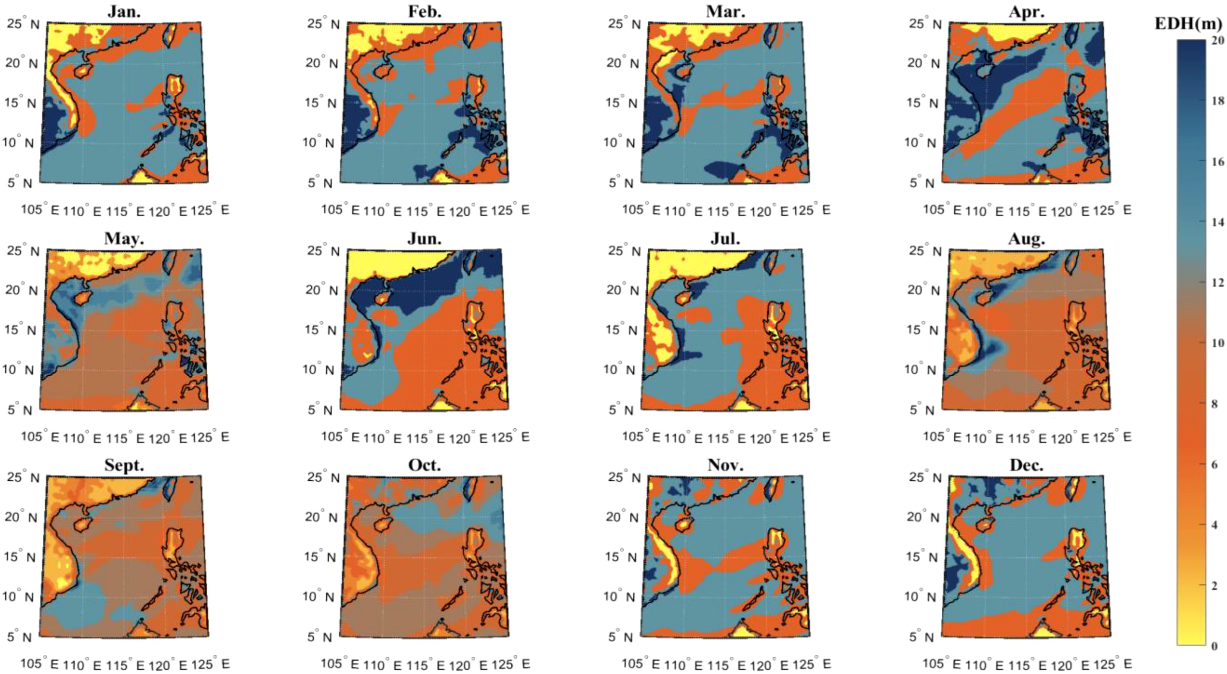
Height map of annual evaporation duct occurrence in the South China Sea.
2.3 Model determination
The ITU-R P.2001 model (hereafter referred to as ITU) is a widely used general ground propagation model for frequencies ranging from 30 MHz to 50 GHz. The International Telecommunication Union proposed the model in 2012 and revised it in 2013, 2015, 2019, 2021, and 2023. This model applies to propagation prediction in the frequency range of 30 MHz to 50 GHz, with propagation distances from 3 to 1000 km, and for time percentages ranging from 0% to 100%. The model consists of the normal propagation close to the surface of the Earth sub-model, the anomalous propagation sub-model, the troposcatter propagation model, and the sporadic-E sub-model. These sub-models consider different propagation mechanisms, including line-of-sight propagation, atmospheric waveguide, tropospheric scattering, and ionospheric scattering. The final predicted loss is obtained by combining the sub-model predictions through their correlations or the Monte Carlo algorithm (International Telecommunication Union (ITU-R), 2023). The radio wave propagation in the modeling area only involves the normal propagation close to the surface of the Earth and troposcatter propagation. Therefore, the model can be expressed using Equation 1.
where Lm represents the climatic loss (meteorological factors), as shown in Equation 2; Lf is the frequency loss, as shown in Equation 3; Ld is the distance loss, as shown in Equation 4; La is the attenuation factor beyond the q% time percentage, as shown in Equation 5; and Lo represents other attenuation losses, as shown in Equation 6.
where Mg represents the meteorological attenuation loss related to the climate zone for the ground; Mt is the meteorological attenuation loss related to the climate zone for the troposphere.
where f represents the frequency (GHz).
where D represents the great-circle distance of the path (km); d is the path distance (km); and θ is the scattering angle (mrad), which is calculated based on d.
where A1 represents the attenuation of the ground exceeding the q% time percentage; A2 represents the attenuation of the troposphere exceeding the q% time percentage.
where Lb represents the Brillouin scattering loss caused by obstacles, Ls represents the Brillouin scattering loss caused by a smooth path profile, and Lh represents the scattering loss caused by the curvature of the Earth’s surface. Gt and Gr are the gains of the transmitting and receiving antennas, respectively, and Y(q) is the probability conversion factor for the loss.
Figure 3 shows a line chart of the deviation (as shown in Equation 7) between the ITU model’s prediction and the measurement.
Figure 3
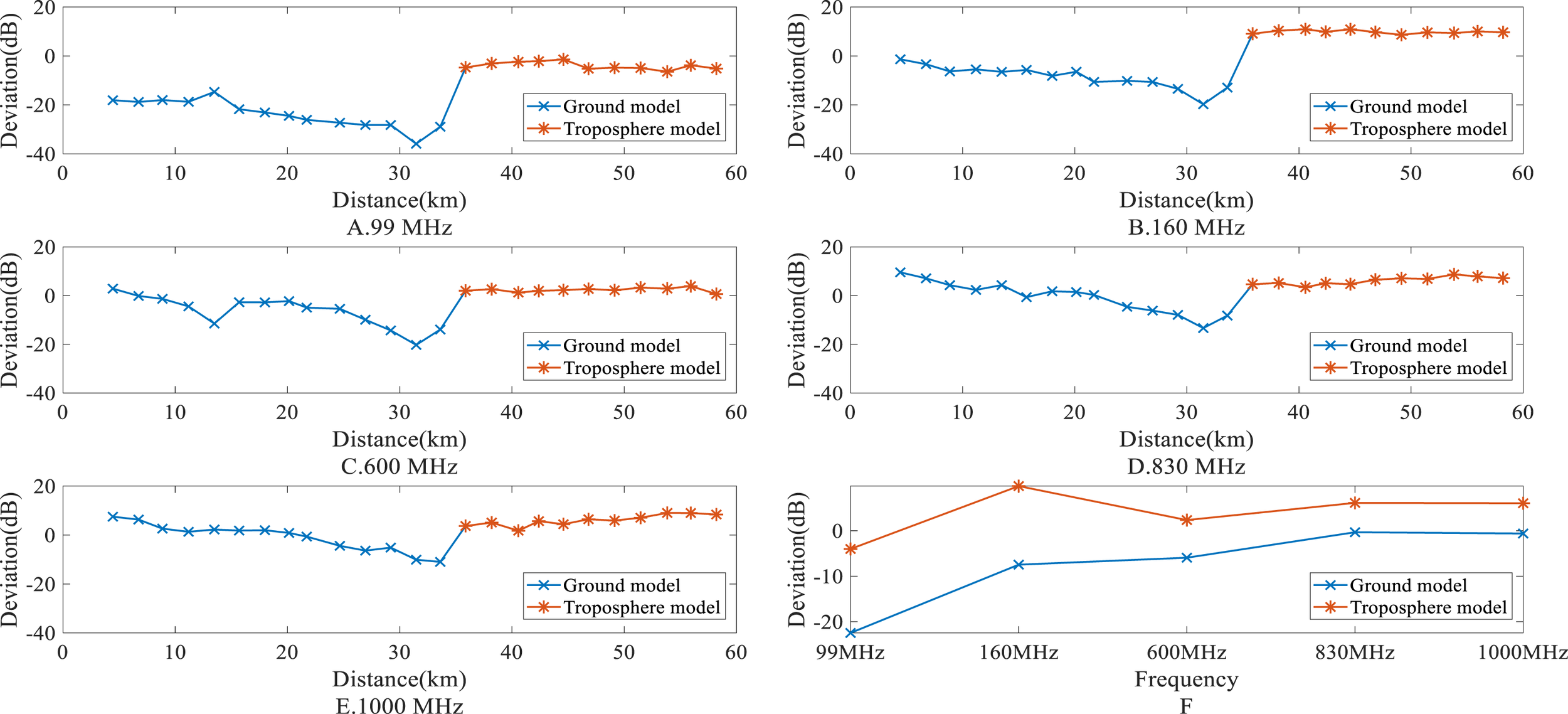
The deviation between the ITU model’s prediction and the measurement. (A) The deviation at 99MHz. (B) The deviation at 160MHz. (C) The deviation at 600MHz. (D) The deviation at 830MHz. (E) The deviation at 1000MHz. (F) Deviation comparison across different frequencies.
From the figure, we can observe that in the distance dimension (Figures 3A-E), the deviation shows a negative slope linear relationship for the normal propagation close to the surface of the Earth model, while the deviation of the troposcatter propagation model exhibits a linear relationship with an approximate zero slope. In the frequency dimension (Figure 3F), the deviations of both sub-models exhibit a logarithmic shift transformation fitting trend.
where L represents the predicted loss from the ITU model, and Lt represents the measured loss.
Based on the above analysis, we use Equation 1 as the foundational model, apply a logarithmic function to correct the frequency loss, and a linear function to correct the distance loss to construct the driving model. The expression is as shown in Equation 8.
where Lf is as shown in Equation 9; Ld is as shown in Equation 10; c1 and c2 are constants.
where a, b, m, n, c1, and c2 are undetermined coefficients. Specifically, a denotes the additional impact of near-ground environments on the frequency dependence of propagation loss, while b denotes the additional frequency dependence introduced by tropospheric conditions. The coefficient m denotes the distance-dependent attenuation factor in near-ground propagation, reflecting the average excess loss per unit distance, whereas c1 serves as a baseline correction term at the beginning of the propagation path, compensating for fixed deviations caused by antenna installation conditions, ground boundary effects, and related factors. Similarly, n represents the distance-dependent attenuation coefficient in tropospheric propagation, describing the cumulative excess loss with increasing distance, and c2 accounts for fixed environmental corrections in tropospheric propagation, compensating for constant deviations due to climatic conditions, antenna configurations, and baseline differences inherent in empirical formulas.
The undetermined coefficients in the proposed driven model characterize the deviations between the measured data and the predictions of the ITU model. Specifically, when these coefficients are optimized to their best-fit values, the predicted path loss of the driven model (Lp) converges to the measured path loss (Lt), as expressed in Equation 11.
By substituting the data of two measured links into Equation 11 and keeping all other propagation parameters identical except for frequency, the value ranges of the undetermined coefficients a and b can be obtained through simultaneous solving, as shown in Equation 12. Similarly, when all parameters except distance are kept the same, the value ranges of the undetermined coefficients m and n can be determined, as expressed in Equation 13.
The constant coefficient c represents the offset. Comparing the deviation between the ITU model predictions and the measured values falls within the range [-35.88,10.88]. Therefore, this interval is the optimization range for the constant coefficient c.
Based on the above procedure, the optimization ranges of all undetermined coefficients in the proposed model were determined, as summarized in Table 2. Subsequently, the model-driven component, represented by Lp is combined with a data-driven component, where a GA is employed to extract features from the measured data. Integrating these two components establishes an empirical propagation loss prediction model for maritime wireless channels.
Table 2
| Undetermined coefficients for | Value |
|---|---|
| a | [-75.16, 3.29] |
| b | [-48.85, -6.76] |
| m | [-5.67, 3.13] |
| n | [-10.05, 26.59] |
| c1&c2 | [-35.88, 10.88] |
Range of undetermined coefficients for the driving model.
2.4 Modeling process
This study leverages measured data and employs the GA as a data-driven approach to optimize the undetermined coefficients in the driven model, thereby establishing a more accurate prediction model. GA is an optimization algorithm inspired by the process of biological evolution in nature, and it is widely applied to solve complex optimization problems (Li et al., 2016). Through iterative evolution and refinement of candidate solutions, GA effectively explores high-dimensional search spaces and is particularly suitable for combinatorial and parameter optimization tasks (Wang et al., 2023c). In GA, the parameters to be optimized are encoded into chromosomes. By performing genetic operations such as selection, crossover, and mutation, GA achieves global optimization while reducing the risk of being trapped in local optima (Abualigah et al., 2021).
Figure 4 illustrates the GA optimization process. First, chromosomes are constructed using the parameters to be optimized: a, b, m, n, c1, and c2. The initial values adopted in this study are used solely as starting points for model training and do not affect the effectiveness of hyperparameter optimization. Based on the initial values and optimization ranges of all frequencies summarized in Table 3, corresponding chromosome individuals and populations are randomly generated, with each parameter initialized within its optimization range. Next, the parameters encoded in each chromosome are substituted into the driven model to calculate the fitness values, thereby assessing the performance of each chromosome.
Figure 4
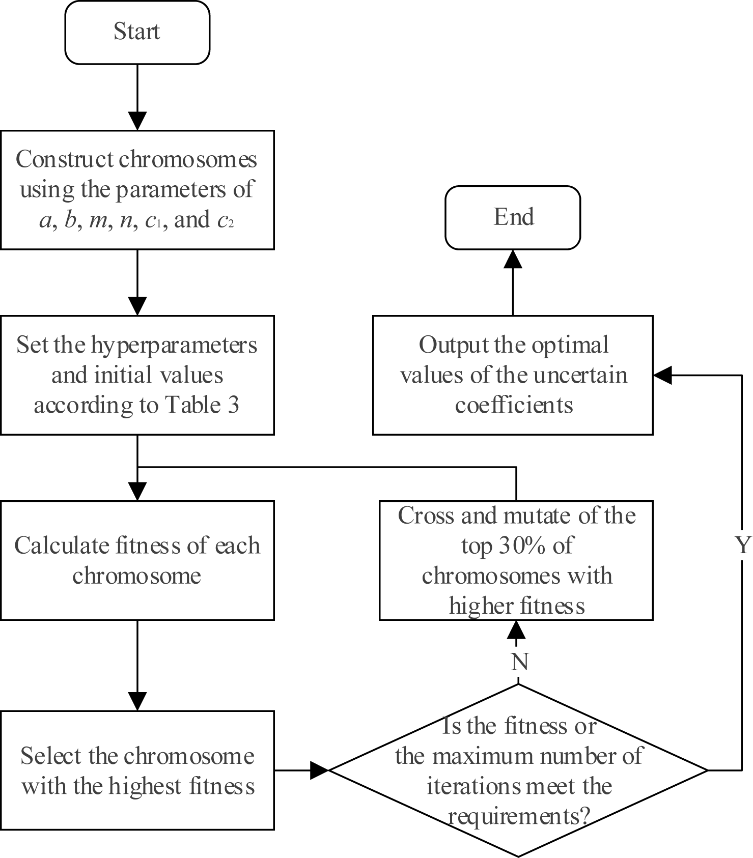
The optimization process of GA.
Table 3
| Hyperparameters | Value | Range |
|---|---|---|
| Population size | 500 | – |
| The number of generations | 500 | |
| The crossover probability | 30% | |
| The mutation probability | 30% | |
| a | 1.12 | Refer to Table 2 |
| b | 6.14 | |
| m | -3.29 | |
| n | -17.41 | |
| c 1&c2 | 0 |
Hyperparameters of GA.
The algorithm then evaluates whether the stopping criteria—defined by either the maximum number of iterations or the convergence of fitness—are satisfied. If the criteria are met, the chromosome with the highest fitness is selected, and the corresponding parameter values are adopted as the final coefficients of the proposed model. Otherwise, the top 30% of chromosomes with higher fitness are preserved for crossover and mutation operations, while the remaining 70% of the population is regenerated within the predefined parameter bounds. This process is iteratively repeated until the termination condition is fulfilled.
3 Result and discussion
3.1 Modeling results and evaluation metrics
The optimal values through the GA optimization process are shown in Table 4. These coefficients represent the best-fit parameters that minimize the deviation between the predicted path loss and the measured data, ensuring the accuracy and reliability of the proposed model. In the following, we will evaluate the performance of the proposed model using objective metrics such as RMSE (denoted as σ) and the improvement percentage (denoted as δ). The specific definitions of these metrics are provided in Equations 14 and 15.
Table 4
| Coefficients | Physical significance | Frequency/MHz | ||||
|---|---|---|---|---|---|---|
| 99 | 160 | 600 | 830 | 1000 | ||
| a | Represents the additional impact of near-ground environments on the frequency dependence of propagation loss | -23.05 | -20.11 | -25.99 | -26.48 | -21.10 |
| m | Denotes the distance-dependent attenuation factor in near-ground propagation, reflecting the average excess loss per unit distance | 0.55 | 0.45 | 0.55 | 0.74 | 0.55 |
| c 1 | Serves as a baseline correction term at the beginning of the propagation path, compensating for fixed deviations due to antenna installation, ground boundary effects, and related factors | -9.68 | -16.13 | -9.68 | -16.13 | -9.68 |
| b | Represents the additional frequency dependence introduced by tropospheric conditions | -14.06 | -14.06 | -19.85 | -19.30 | -16.82 |
| n | Represents the distance-dependent attenuation coefficient in tropospheric propagation, describing the cumulative excess loss with increasing distance | 0.13 | 0.03 | 0.06 | 0.03 | 0.06 |
| c 2 | Accounts for fixed environmental corrections in tropospheric propagation, compensating for constant deviations due to climatic conditions, antenna configurations, and baseline differences inherent in empirical formulas | -16.13 | -22.58 | -9.68 | -9.68 | -9.68 |
The optimal value of the undetermined coefficient.
where Lm is the measured path loss value, Lp is the path loss value predicted by the model, and N is the number of observation points at each frequency.
where σi represents the RMSE between the ITU model and the measured value, while σp denotes the RMSE between the predictions of the proposed model and the measured values.
3.2 Comparative analysis of model predictive performance
Figure 5 shows a comparison between the measurement and prediction. From Figures 5A-E, it can be observed that both the ITU and the proposed (hereafter referred to as PRO) models reflect the trend of the measured losses. However, the PRO model exhibits better consistency with the measured losses, indicating superior prediction accuracy of the PRO model. In the distance dimension, the ITU model demonstrates an increasing prediction accuracy as the distance increases. As observed in Figure 5F, with the increase in frequency, the prediction accuracy of the ITU model also improves, indicating that the ITU model is influenced by both distance and frequency. The PRO model demonstrates greater stability than the ITU model in both the distance and frequency dimensions, and its prediction accuracy significantly outperforms that of the ITU model. In addition, it can be observed that the path loss of the ITU and PRO models around 34 km shows obvious nonlinearity. The specific reason is that the ITU-R P.2001 model comprises multiple propagation sub-models. Specifically, sub-model 1 is applied before 34km, while sub-model 3 is adopted for distances greater than 34 km (the method for combining these sub-models is described in Appendix J of (International Telecommunication Union (ITU-R), 2023)). The transformation between sub-models yields a noticeable nonlinearity in the prediction curve.
Figure 5
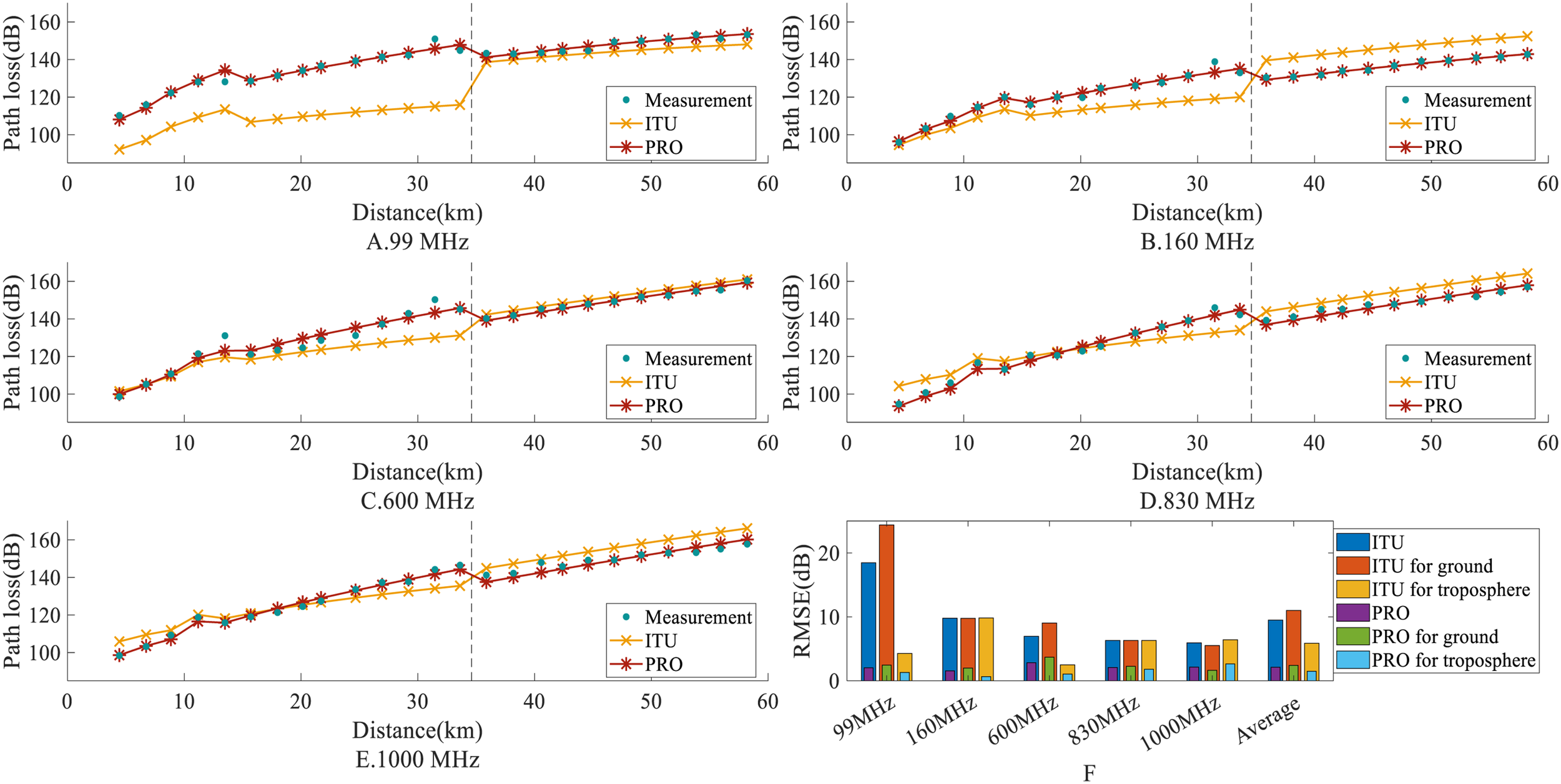
Comparison of measured and predicted path loss. (A) Measured and predicted path loss at 99MHz. (B) Measured and predicted path loss at 160MHz. (C) Measured and predicted path loss at 600MHz. (D) Measured and predicted path loss at 830MHz. (E) Measured and predicted path loss at 1000MHz. (F) RMSE of all frequencies.
Figure 6A shows the overall comparison of the RMSE between the ITU and the PRO models across different frequencies. It can be seen that the RMSE of the PRO model is significantly lower than that of the ITU model, with the average RMSE across all frequencies reduced by 7.37dB compared to the ITU model. Among them, the 99MHz band shows the largest reduction of 16.44dB, while the 600MHz band shows the smallest reduction of 4.12dB.
Figure 6
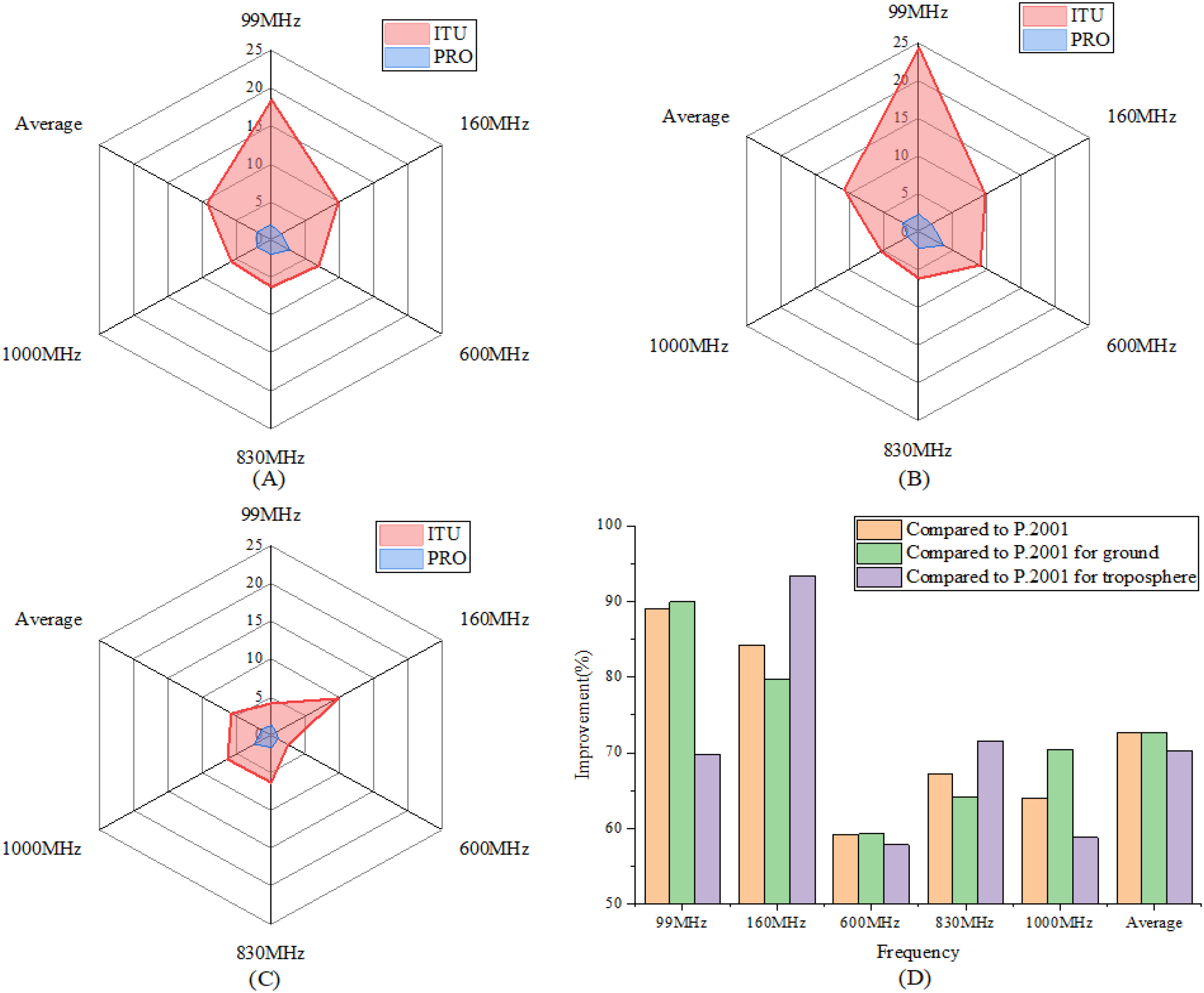
RMSE comparison between ITU and PRO models. (A) Overall comparison. (B) For the normal propagation close to the surface of the Earth. (C) For the troposcatter propagation. (D) The Improvement Percentage.
Figures 6B, C show the radar chart comparison of the ITU and PRO sub-models. The overall shapes of the ITU and PRO radar charts are closer to those of normal propagation close to the surface of the Earth, indicating that the model prediction error mainly originates from this sub-model. The RMSE (Rg) of the ITU normal propagation close to the surface of the Earth model decreases significantly with increasing frequency, indicating that this sub-model is highly influenced by frequency. At lower frequencies, the ITU model exhibits a relatively high Rg, reaching as much as 21.81dB at 99MHz. The PRO model effectively addresses this issue, reducing the maximum Rg to just 3.68dB. The PRO model not only significantly improves the accuracy but also enhances the stability in frequencies. The average RMSE of the ITU troposcatter propagation sub-model across all frequencies is 5.87dB.
In contrast, the PRO troposcatter propagation sub-model achieves a significantly lower average RMSE of just 1.49dB, representing a reduction of 4.38dB compared to the ITU model.
Figure 6D presents the improvement percentages of the PRO model compared to the ITU model. The figure shows that the PRO model and its sub-models exhibit improvements exceeding 57% across all frequencies relative to the ITU model. Specifically, the average improvement percentages for the PRO model, the normal propagation close to the surface of the Earth sub-model, and the troposcatter propagation sub-model are 72.73%, 72.71%, and 70.28%, respectively. The PRO model and the normal propagation close to the surface of the Earth sub-model show the greatest improvements at the 99 MHz frequency band, with improvement percentages of 89.04% and 89.95%, respectively. The troposcatter propagation sub-model achieves its highest improvement at the 160 MHz frequency band, with an improvement percentage of 93.37%. Although the improvements are smallest at the 600 MHz frequency band, the PRO model and its sub-models still achieve significant enhancements, with improvement percentages of 59.20%, 59.28%, and 57.86%, respectively.
Figure 7 shows the boxplot comparison of each model and Table 5 shows the RMSE of each model at each frequency. It can be observed that the free-space propagation (FSP) model exhibits the largest RMSE, followed by the ITU model, the two-ray (TR) model, and the PRO model, which has the smallest RMSE. Both the FSP and ITU models demonstrate strong spatial correlation, with RMSE decreasing as frequency increases; the ITU model clearly outperforms the FSP model in terms of RMSE. The TR and PRO models show relatively stable predictions across frequency bands, with the PRO model achieving higher prediction accuracy than the TR model.
Figure 7
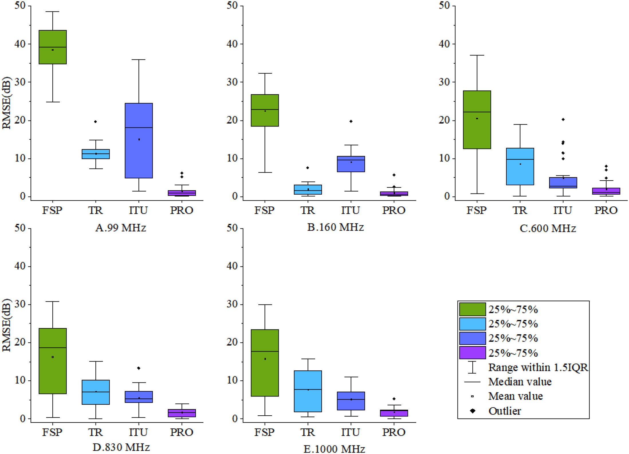
Comparison of the three models. (A) Box plot of the RMSE at 99MHz. (B) Box plot of the RMSE at 160MHz. (C) Box plot of the RMSE at 600MHz. (D) Box plot of the RMSE at 830MHz. (E) Box plot of the RMSE at 1000MHz.
Table 5
| Model\ Frequency |
99 MHz | 160 MHz | 600 MHz | 830 MHz | 1000 MHz | Average |
|---|---|---|---|---|---|---|
| FSP | 39.01 | 23.36 | 22.89 | 18.64 | 18.31 | 24.44 |
| TW | 11.56 | 2.58 | 10.28 | 8.36 | 9.24 | 8.40 |
| ITU | 18.47 | 9.80 | 6.96 | 6.31 | 5.93 | 9.49 |
| PRO | 2.03 | 1.55 | 2.84 | 2.07 | 2.14 | 2.13 |
The RMSE of each model at each frequency.
Specifically, the FSP model has an average RMSE of 24.44 dB across frequencies, with the mean lower than the median, indicating overall larger prediction errors and lower model accuracy. The TR model has an average RMSE of 8.40 dB, with mean and median coinciding, suggesting a roughly symmetric distribution without significant skewness and relatively stable predictions. The ITU model has an average RMSE of 9.49 dB. At 600 MHz and 1000 MHz, the ITU model’s mean RMSE exceeds the median, indicating the presence of relatively large prediction errors at these frequencies. Moreover, at the 1000 MHz band, the ITU model exhibits more outliers, reflecting poorer stability in this band. In contrast, the PRO model has an average RMSE of 2.13 dB. It shows significantly smaller box sizes across all frequency bands, with values concentrated near zero, suggesting more concentrated RMSE values and smaller overall prediction errors. Additionally, the mean and median of the PRO model coincide across all frequencies, indicating symmetric prediction errors that closely align with a normal distribution, consistent with the statistical characteristics of large-scale propagation predictions.
4 Conclusion
This study proposed a high-precision empirical maritime channel model by integrating data-driven and model-driven approaches. First, a theory-driven model with undetermined coefficients was developed to describe the propagation mechanisms of the target maritime area based on the ITU-R P.2001 framework. Then, a data-driven component was established by employing a GA to extract environmental features from measured data and optimize the model coefficients. By combining these two approaches, a robust hybrid modeling framework was constructed. Extensive validation demonstrated that the proposed model achieves a mean RMSE of 2.13dB, corresponding to a 72.73% improvement in prediction accuracy compared with the ITU-R P.2001 model. These results highlight that the integration of theoretical modeling and intelligent data-driven optimization can significantly enhance the accuracy and stability of maritime path loss prediction.
The proposed model provides a practical tool for maritime wireless system design and planning, supporting applications such as maritime broadband communication, ship-to-ship and ship-to-shore connectivity, and the extension of future 6G networks over ocean environments. Moreover, the methodology offers a generalizable framework that can be extended to other challenging environments beyond maritime scenarios.
Statements
Data availability statement
The original contributions presented in the study are included in the article/Supplementary Material. Further inquiries can be directed to the corresponding author/s.
Author contributions
YH: Data curation, Formal analysis, Investigation, Software, Validation, Visualization, Writing – original draft. ZW: Data curation, Methodology, Validation, Visualization, Writing – original draft, Writing – review & editing. HZ: Conceptualization, Investigation, Resources, Supervision, Visualization, Writing – review & editing. ZC: Data curation, Software, Supervision, Validation, Writing – review & editing. JM: Data curation, Visualization, Writing – review & editing. JW: Conceptualization, Funding acquisition, Project administration, Resources, Writing – review & editing. CY: Funding acquisition, Investigation, Resources, Writing – review & editing.
Funding
The author(s) declared that financial support was received for this work and/or its publication. This work was supported in part by the National Natural Science Foundation of China 62031008.
Conflict of interest
ZC was employed by company China Mobile Construction Co., Ltd.
The remaining author(s) declared that this work was conducted in the absence of any commercial or financial relationships that could be construed as a potential conflict of interest.
Generative AI statement
The author(s) declared that generative AI was not used in the creation of this manuscript.
Any alternative text (alt text) provided alongside figures in this article has been generated by Frontiers with the support of artificial intelligence and reasonable efforts have been made to ensure accuracy, including review by the authors wherever possible. If you identify any issues, please contact us.
Publisher’s note
All claims expressed in this article are solely those of the authors and do not necessarily represent those of their affiliated organizations, or those of the publisher, the editors and the reviewers. Any product that may be evaluated in this article, or claim that may be made by its manufacturer, is not guaranteed or endorsed by the publisher.
Supplementary material
The Supplementary Material for this article can be found online at: https://www.frontiersin.org/articles/10.3389/fmars.2026.1755348/full#supplementary-material
References
1
Abualigah L. Diabat A. Mirjalili S. Abd Elaziz M. Gandomi A. H. (2021). The arithmetic optimization algorithm. Comput. Methods Appl. Mechanics Eng.376, 113609. doi: 10.1016/j.cma.2020.113609
2
Afape J. O. Willoughby A. A. Sanyaolu M. E. Obiyemi O. O. Moloi K. Jooda J. O. et al . (2024). Improving millimetre-wave path loss estimation using automated hyperparameter-tuned stacking ensemble regression machine learning. Results Eng.22, 102289. doi: 10.1016/j.rineng.2024.102289
3
Erunkulu O. O. Gwebu T. I. Zungeru A. M. Lebekwe C. Modisa M. (2023). Propagation channel characterization for mobile communication based on measurement campaign and simulation. Results Eng.20, 101620. doi: 10.1016/j.rineng.2023.101620
4
He Y. Zhang S. Liu W. Chen R. Zhao M. Li K. et al . (2022). A novel 3D non-stationary maritime wireless channel model. IEEE Trans. Commun.70, 2102–2116. doi: 10.1109/TCOMM.2021.3134275
5
Hu X. Wang Y. Xu Z. Li J. Zhang T. Chen L. et al . (2024). Performance analysis of end-to-end LEO satellite-aided shore-to-ship communications: A stochastic geometry approach. IEEE Trans. Wireless Commun.23, 11753–11769. doi: 10.1109/TWC.2024.3388810
6
Huang S. Zhao X. Liu J. Wang Y. Li H. Chen M. et al . (2024). Comparative study of VPE-driven CNN models for radio wave propagation modeling in tunnels. IEEE Trans. Antennas Propagation72, 9421–9436. doi: 10.1109/TAP.2024.3478818
7
International Telecommunication Union (ITU-R) . (2019). Recommendation ITU-R P.525-4: Calculation of free-space attenuation (Geneva, Switzerland: ITU).
8
International Telecommunication Union (ITU-R) . (2023). A general purpose wide-range terrestrial propagation model in the frequency range 30 MHz to 50 GHz (Recommendation ITU-R P.2001-5) (Geneva, Switzerland: ITU).
9
Lee J.-H. Choi J. Lee W.-H. Choi J.-W. Kim S.-C. (2017). Measurement and analysis on land-to-ship offshore wireless channel in 2.4 GHz. IEEE Wireless Commun. Lett.6, 222–225. doi: 10.1109/LWC.2017.2662380
10
Li L. Wu Z.-S. Lin L.-K. Zhang R. Zhao Z.-W. (2016). Study on the prediction of troposcatter transmission loss. IEEE Trans. Antennas Propagation64, 1071–1079. doi: 10.1109/TAP.2016.2515125
11
Majid S. I. Majid S. I. Ali H. Khan S. Gohar N. Al-Rasheed A. (2024). Optimizing cell selection for data services in mm-waves spectrum through enhanced extreme gradient boosting. Results Eng.21, 101868. doi: 10.1016/j.rineng.2024.101868
12
Mezaal M. T. Aripin N. B. M. Othman N. S. Sallomi A. H. (2024). Empirical modelling of dust storm path attenuation for 5G mmWave. Results Eng.22, 102092. doi: 10.1016/j.rineng.2024.102092
13
Seretis A. Sarris C. D. (2021). An overview of machine learning techniques for radiowave propagation modeling. IEEE Trans. Antennas Propagation70, 3970–3985. doi: 10.1109/TAP.2021.3098616
14
Wang J. Hao Y. Wu Z. Shi Y. Yang C. (2024b). A broadcast map constructing method based on the LSTM and assimilation theory. IEEE Trans. Broadcasting70, 924–934. doi: 10.1109/TBC.2024.3434536
15
Wang J. Hao Y. Yang C. (2023a). An entropy weight-based method for path loss predictions for terrestrial services in the VHF and UHF bands. Radio Sci.58, e2023RS010123. doi: 10.1029/2023RS007769
16
Wang J. Hao Y. Yang C. (2023b). A comprehensive prediction model for VHF radio wave propagation by integrating entropy weight theory and machine learning methods. IEEE Trans. Antennas Propagation71, 6249–6254. doi: 10.1109/TAP.2023.3266840
17
Wang J. Hao Y. Yang C. (2023c). The current progress and future prospects of path loss model for terrestrial radio propagation. Electronics12, 4959. doi: 10.3390/electronics12244959
18
Wang J. Wu Z. Hao Y. Yang C. (2024c). Broadcasting map construction method based on particle swarm optimization-assisted support vector machine integrated model. IEEE Trans. Antennas Propagation72, 6638–6651. doi: 10.1109/TAP.2024.3421280
19
Wang J. Yang C. Yan N. N. (2021). Study on digital twin channel for the B5G and 6G communication. Chin. J. Radio Science 36(3)340–348, 385. doi: 10.12265/j.cjors.2020240
20
Wang C. Ai B. He R. Yang M. Zhou S. Yu L. (2024a). Channel path loss prediction using satellite images: A deep learning approach. IEEE Trans. Mach. Learn. Commun. Networking2, 1357–1368. doi: 10.1109/TMLCN.2024.3454019
21
Wu Z. Zhao Y. Yang C. Shi Y. Hao Y. Sun J. et al . (2024). Applicability of ITU-R P.2001 recommendation in the FAST radio quiet zone. Chin. J. Radio Sci.39, 658–664. doi: 10.12265/j.cjors.2024043
22
Xu J. Kishk M. A. Alouini M. S. (2023). Space-air-ground-sea integrated networks: Modeling and coverage analysis. IEEE Trans. Wireless Commun.22, 6298–6313. doi: 10.1109/TWC.2023.3241341
23
Yang M. Chen L. Zhao J. Li H. Wu K. Zhang R. et al . (2023b). AI-enabled data-driven channel modeling for future communications. IEEE Commun. Magazine62, 112–118. doi: 10.1109/MCOM.019.2300072
24
Yang C. Shi Y. Wang J. Ma J. (2023a). ELM-based impact analysis of meteorological parameters on the radio transmission of X-band over the Qiongzhou Strait of China. China Commun.20, 244–256. doi: 10.23919/JCC.fa.2022-0687.202312
25
You X. Wang C. Huang L. Gao X. Zhang Z. Wang M. et al . (2021). Towards 6G wireless communication networks: Vision, enabling technologies, and new paradigm shifts. Sci. China Inf. Sci.64, 110301. doi: 10.1007/s11432-020-2955-6
26
Yu S. (2024). Research on spread-spectrum communication system under ionospheric scattering channel (Xi’an, China: Xidian University).
27
Zhang H. Zhou T. Xu T. Cheng M. Hu H. (2024). Field measurement and channel modeling around Wailingding Island for maritime wireless communication. IEEE Antennas Wireless Propagation Lett.23, 1934–1938. doi: 10.1109/LAWP.2024.3374788
28
Zhang Q. Zheng Y. Yuan Q. Song M. Yu H. Xiao Y. (2023). Hyperspectral image denoising: From model-driven, data-driven, to model-data-driven. IEEE Trans. Neural Networks Learn. Syst.35, 13143–13163. doi: 10.1109/TNNLS.2023.3278866
Summary
Keywords
data-model driven, maritime radio wave propagation, path loss, VHF/UHF, wireless communications
Citation
Hao Y, Wu Z, Zhao H, Chen Z, Ma J, Wang J and Yang C (2026) Measured data and empirical model jointly driven prediction for path loss of VHF and UHF communication in the South China Sea. Front. Mar. Sci. 13:1755348. doi: 10.3389/fmars.2026.1755348
Received
27 November 2025
Revised
10 January 2026
Accepted
19 January 2026
Published
04 February 2026
Volume
13 - 2026
Edited by
Leonid Chernogor, V. N. Karazin Kharkiv National University, Ukraine
Reviewed by
Shuangde Li, Nanjing University of Posts and Telecommunications, China
Xinjin Lu, National University of Defense Technology, China
Updates
Copyright
© 2026 Hao, Wu, Zhao, Chen, Ma, Wang and Yang.
This is an open-access article distributed under the terms of the Creative Commons Attribution License (CC BY). The use, distribution or reproduction in other forums is permitted, provided the original author(s) and the copyright owner(s) are credited and that the original publication in this journal is cited, in accordance with accepted academic practice. No use, distribution or reproduction is permitted which does not comply with these terms.
*Correspondence: Jing Wang, wantjoy@sina.com; Cheng Yang, ych2041@tju.edu.cn
†These authors have contributed equally to this work and share first authorship
Disclaimer
All claims expressed in this article are solely those of the authors and do not necessarily represent those of their affiliated organizations, or those of the publisher, the editors and the reviewers. Any product that may be evaluated in this article or claim that may be made by its manufacturer is not guaranteed or endorsed by the publisher.