Abstract
Estuarine topography influences hydrodynamics and salinity intrusion. The most significant feature of salinity intrusion in the Yangtze River Estuary is the salt-spilling-over (SSO) into the South Branch from the North Branch (NB), which affects the utilization of freshwater resources in the South Branch where three reservoirs were built. The topography in different decades from the 1950s to the 2020s was collected, and a numerical model was adopted to simulate the topography changes on salinity intrusion and SSO. From the 1950s to the 2020s, the topography of the Yangtze River Estuary changed greatly, especially in the NB. The channel area of the NB decreased by 55.56%, and its channel volume decreased by 57.57%. The numerical simulation results showed that the evolution of salinity intrusion in the NB and SSO experienced weakening–enhancing–weakening processes. The NB was covered by high-salinity water and experienced the SSO in the 1950s. The SSO distinctly weakened in the 1970s and 1980s, greatly enhanced in the 1990s, reached its most severe level in the 2000s, and significantly weakened in the 2010s and 2020s. From the 1950s to the 2020s, the tidal prism of the NB constantly decreased, with a reduction of 62.32% during spring–neap tide. The variations in the net water flux, net salt flux, and water diversion ratio in the upper section of the NB were consistent with the evolution processes of SSO. The evolution mechanisms of the salinity intrusion and SSO were elucidated in view of changes in the estuarine topography and dynamic factors.
1 Introduction
Estuarine regions hold critical ecological and economic significance globally, supporting dense populations and intense economic activity (Delgado et al., 2017; Chen et al., 2024; Jung et al., 2024). A key challenge for estuarine sustainability is salinity intrusion, which threatens freshwater security for human settlements and economic hubs (Mekonnen and Hoekstra, 2016; Jumain et al., 2022; Aziz and Tarya, 2024; Li et al., 2024). In multi-branch estuaries, this issue is compounded by saltwater spillover dynamics, where saltwater from one branch intrudes into adjacent branches, exacerbating freshwater scarcity (Ge et al., 2022; Yang et al., 2023). Previous studies have established short-term drivers of salinity intrusion, such as tides, river discharge, wind, and mixing. River discharge determines freshwater influx and seaward transport, tides drive landward salt transport via flood currents and vertical mixing, and ebb currents export freshwater seaward (Pritchard, 1952; Zhang et al., 2023; Hlaing et al., 2024). Local and remote winds regulate estuarine circulation through localized drag and remote alongshore water transport, altering estuarine salinity intrusion (Zhu et al., 2020; Scroccaro et al., 2023; Tao et al., 2024; Ma et al., 2025). Changes in topography influence salinity intrusion by changing estuarine hydrodynamics, such as tidal prisms, flow partitioning, tidal currents and estuarine circulation (Guo et al., 2022; Kolb et al., 2022; Kwak et al., 2023; Yang et al., 2023). However the long-term control of topographic evolution on saltwater spillover dynamics remains poorly quantified, particularly in large anthropogenically modified systems like the Yangtze River Estuary (Chen et al., 2019; Guo et al., 2022). This knowledge gap limits predictive capacity for freshwater resource management under ongoing morphological changes.
The Yangtze River is the third-largest river in the world and discharges vast amounts of freshwater (9.24×10¹¹ m3) into the East China Sea each year (Shen et al., 2003). The Qingcaosha, Dongfengxisha, and Chenhang estuarine reservoirs were constructed to meet the freshwater demand for Shanghai (Figure 1), which is an international metropolis near the Yangtze River Estuary that has 24.8 million residents. These estuarine reservoirs are frequently affected by salinity intrusion. As a multi- bifurcated estuary, its most significant feature is the water-spilling-over (WSO) and salt-spilling-over (SSO) into the South Branch (SB) from the North Branch (NB) (Yang et al., 2023; Ge et al., 2022; Lyu and Zhu, 2018; Wang and Ge, 2025). The reservoirs in the SB suffer the frontal salinity intrusion and the SSO.
Figure 1
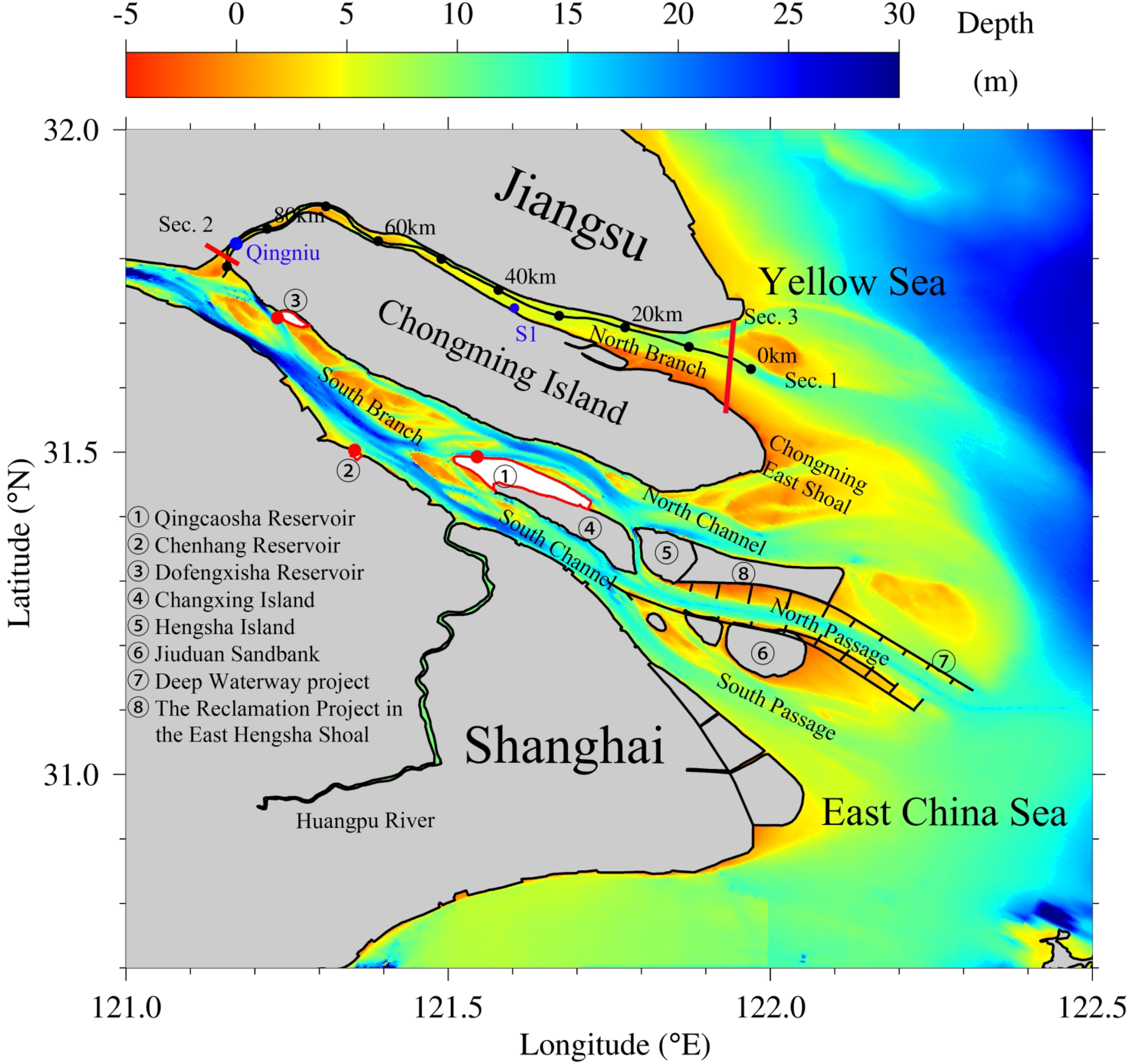
Topography of the Yangtze River Estuary. White areas indicate the locations of the reservoirs. Black line: Sec. 1 is the longitudinal section along the NB. Red line: Sec. 2 and Sec. 3 are the transverse sections at the upstream and downstream, respectively, of the NB. Blue dots: S1 is the model output site of elevation; Qingniu are ocean stations used for model validation.
Previous studies have shown that the topography changes influence the salinity intrusion in the Yangtze River Estuary (Chen et al., 2019; Lyu and Zhu, 2018). These studies were conducted on a relatively short time scale. In this study, we collect the shoreline and water depth data from the 1950s to the 2020s (include 1950s, 1970s, 1980s, 1990s, 2000s, 2010s, 2020s), which is a relatively large time scale, to analyze the topography changes occurring in each decade; in addition, we focus on the evolution of SSO in each decade through numerical simulations. This research holds significant scientific value for advancing the understanding of salinity intrusion dynamics in large multi-branched estuaries and provides critical insights into safeguarding freshwater security in estuaries.
2 Methods
2.1 Numerical model settings
This study applies the numerical model ECOM-si (Blumberg and Mellor, 1987), which was improved to better simulate hydrodynamics and material transport (Wu and Zhu, 2010). Extensive calibrations, validations and applications were conducted in the Yangtze River Estuary, and the results showed that the model could correctly simulate hydrodynamics and salinity intrusion (Yang et al., 2023; Lyu and Zhu, 2018; Wu et al., 2023; Zhu et al., 2020). The model adopted a curvilinear nonorthogonal mesh in the horizontal and σ coordinates in the vertical, covering the Yangtze River Estuary and adjacent seas from 27.5°N to 33.5°N and 117.5°E (Datong hydrologic station, the tidal limit during the dry season) to 125°E (Figure 2a). The highest grid resolution of 100 m is in the difluence of the NB and SB. The computational domains were consistent in all decades (1950s–2020s), with local grid adjustments being made according to changing shorelines inside the estuary (Figures 2b-h). The open sea boundary of the model was specified by tidal elevation and residual elevation. The upstream boundary was driven by river discharge measured at the Datong hydrologic station. The detailed configurations of open sea and river boundary conditions, wind field, and initial condition of salinity can be referred to in literature (Ma and Zhu, 2022).
Figure 2
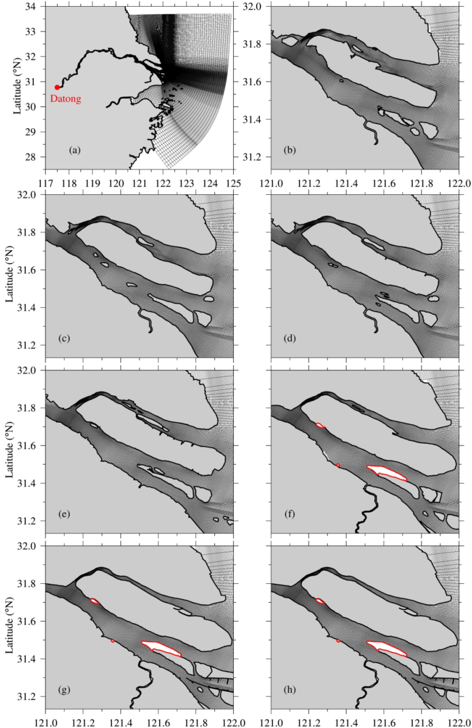
Model calculation domain and curvilinear grids (a). Grids matching the coastlines in the 1950s (b), 1970s (c), 1980s (d), 1990s (e), 2000s (f), 2010s (g) and 2020s (h) in the Yangtze River Estuary.
This study primarily focuses on the influences of topography changes on the evolution of salinity intrusion in the North Branch. To isolate the effects of topographic variations and exclude interference from other factors, we employed long-term monthly mean river discharge and wind data in the model setup. We acknowledge this approach introduces a potential limitation in capturing inter-annual variability and its possible impacts on the results. The simulations began from 1 December 2024 to 1 February 2025, with the first two months allocated for model adjustment and stabilization. The analysis was focused on February data. The river discharge adopts the long-term monthly means (1950–2025) of 14081, 11587 and 12378 m3/s in December, January and February, respectively. The monthly mean of the wind field from 2004 to 2024 was adopted.
2.2 Model validation
The numerical model employed in this study has been thoroughly validated. To further confirm the model’ s reliability, validation was performed using observed elevation and salinity in February 2025. Correlation coefficient, root mean square error, and skill score were employed to evaluate the model performance. The skill score was introduced as a statistical metric to describe the degree to which the observed deviations from the observed mean correspond to the simulated derivations from the observed mean. It classified the model results into four categories to evaluate model performance according to the SS: > 0.65, excellent; 0.5-0.65, very good; 0.2-0.5, good; and <0.2, poor (Murphy, 1988).
The validation results for elevation and salinity at Qingniu station in February 2025 further confirm the reliability of the model (Figure 3). The simulated salinity accurately captured the variation of the salinity with tidal cycles, and the simulated elevation aligned almost perfectly with observed data. For salinity and elevation, the correlation coefficients reached 0.99 and 0.98, root mean square errors were 0.06 and 0.65 psu, and skill scores attained 0.99 and 0.97, respectively.
Figure 3
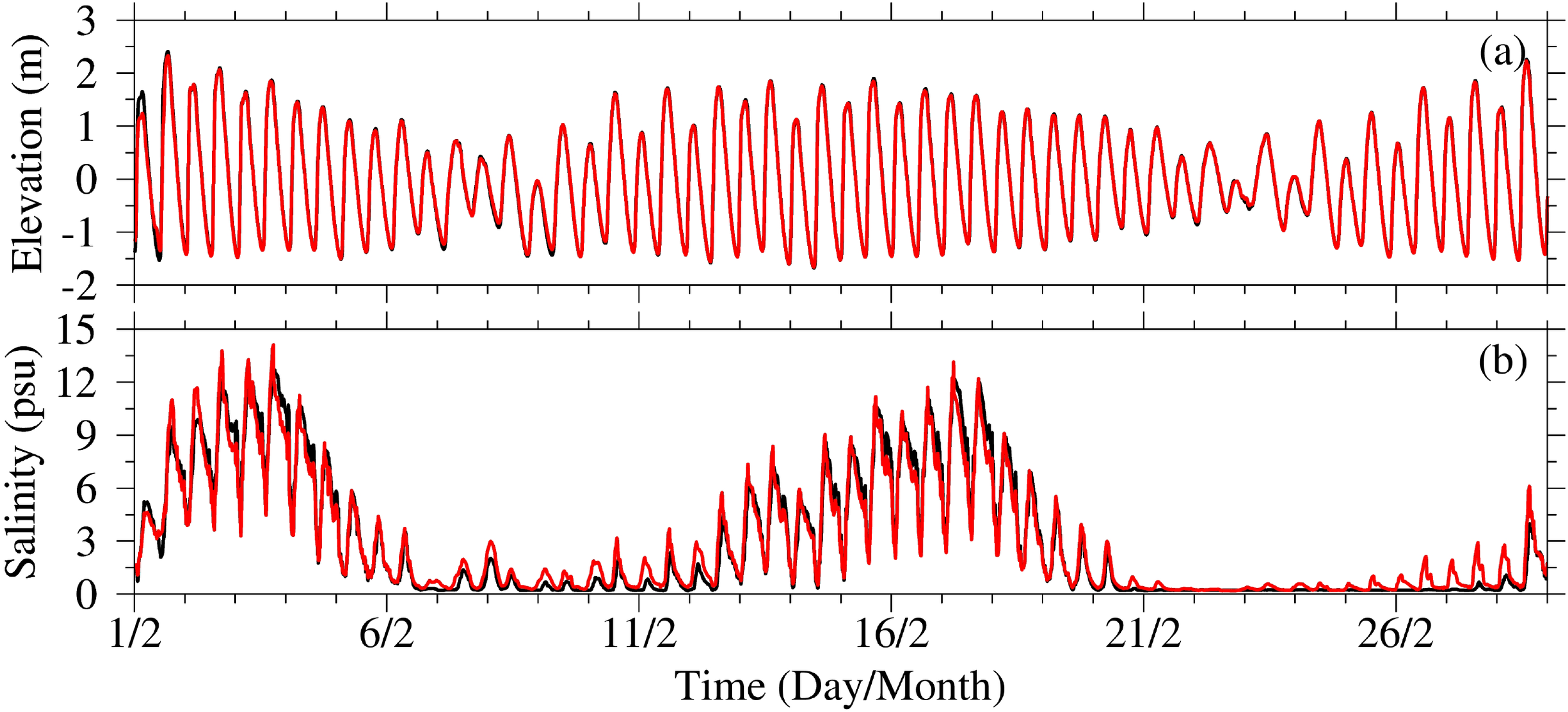
Comparison between the observed (black) and modeled (red) elevation (a) and salinity (b) at the Qingniu station in February 2025.
3 Results
3.1 Topography evolution of the estuary
The topography of the Yangtze River Estuary in the 1950s, 1970s, 1980s, 1990s, 2000s, and 2010s are shown in Figure 4, and the topography in the 2020s is shown in Figure 1. In the 1950s (Figure 4a), the NB was wide, especially at the difluence between the NB and SB, and the Yonglongsha shoal was present in the middle section. Changxing Island had not yet formed; it has had only several shoals. In the 1970s (Figure 4b), the island at the difluence between the NB and SB merged into the west shoreline, and the upper end of the NB became narrower. Then, Changxing Island formed. The Jiuduan Sandbank became increasingly enlarged, dividing the South Channel into the North Passage and South Passage and forming a three-level difluence and four outlets pattern (Shen et al., 2003; Zhang et al., 2011). In the 1980s (Figure 4c), the Yonglongsha shoal developed into the Xinglongsha shoal in the NB. In the 1990s (Figure 4d), the Xinglongsha shoal was prolonged, and the Xincunsha and Lingdiansha appeared upstream. The Jiuduansha Sandbank increased between the North Passage and South Passage. In the 2000s (Figure 4e), the Xinglongsha shoal merged into Chongming Island, the Lingdiansha shoal merged with the north shoreline, and the upper end of the NB became increasingly narrow. Major projects, such as the deep Waterway Project in the North Passage and the Nanhui Shoal reclamation project, were conducted. In the 2010s (Figure 4f), the Xincunsha shoal was reclaimed and merged into Chongming Island. Major projects, such as the Qingcaosha Reservoir, the largest estuarine reservoir, and the reclaimed new land on the Eastern Hengsha Shoal, were completed. In the 2020s (Figure 1), the southern side of the lower section and upper end of the NB became significantly shallower than before. The shoreline changes in the Yangtze River Estuary from the 1950s to the 2020s revealed that the most significant shoreline change occurred in the NB (Figure 5). The NB became increasingly narrow, especially on the southern shoreline in the lower section and at the upper end of the NB.
Figure 4
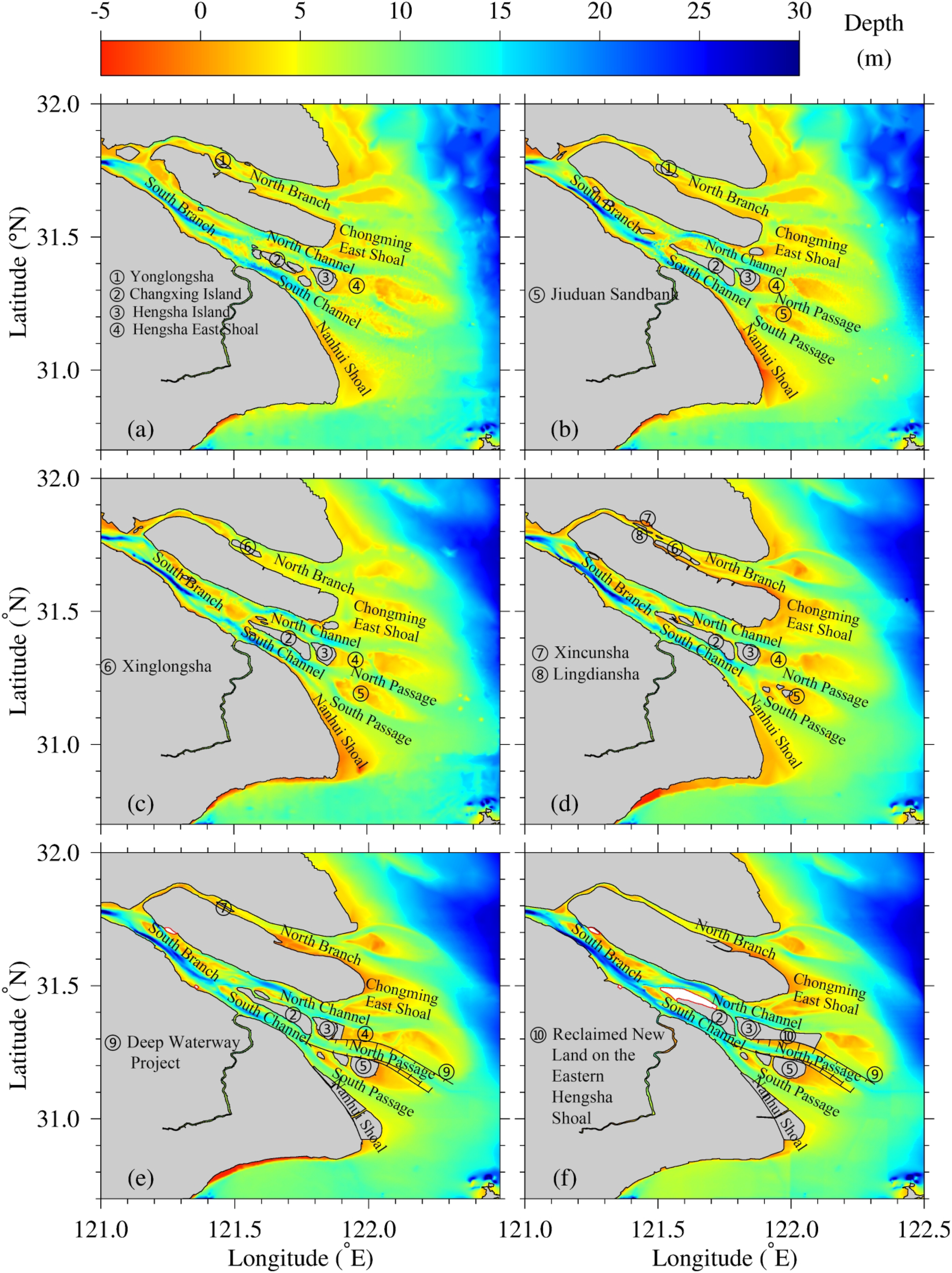
Topography of the Yangtze River Estuary in the 1950s (a), 1970s (b), 1980s (c), 1990s (d), 2000s (e), and 2010s (f). Topography in the 2020s is shown in Figure 1. Shoals and major estuarine projects in different decades were labelled.
Figure 5
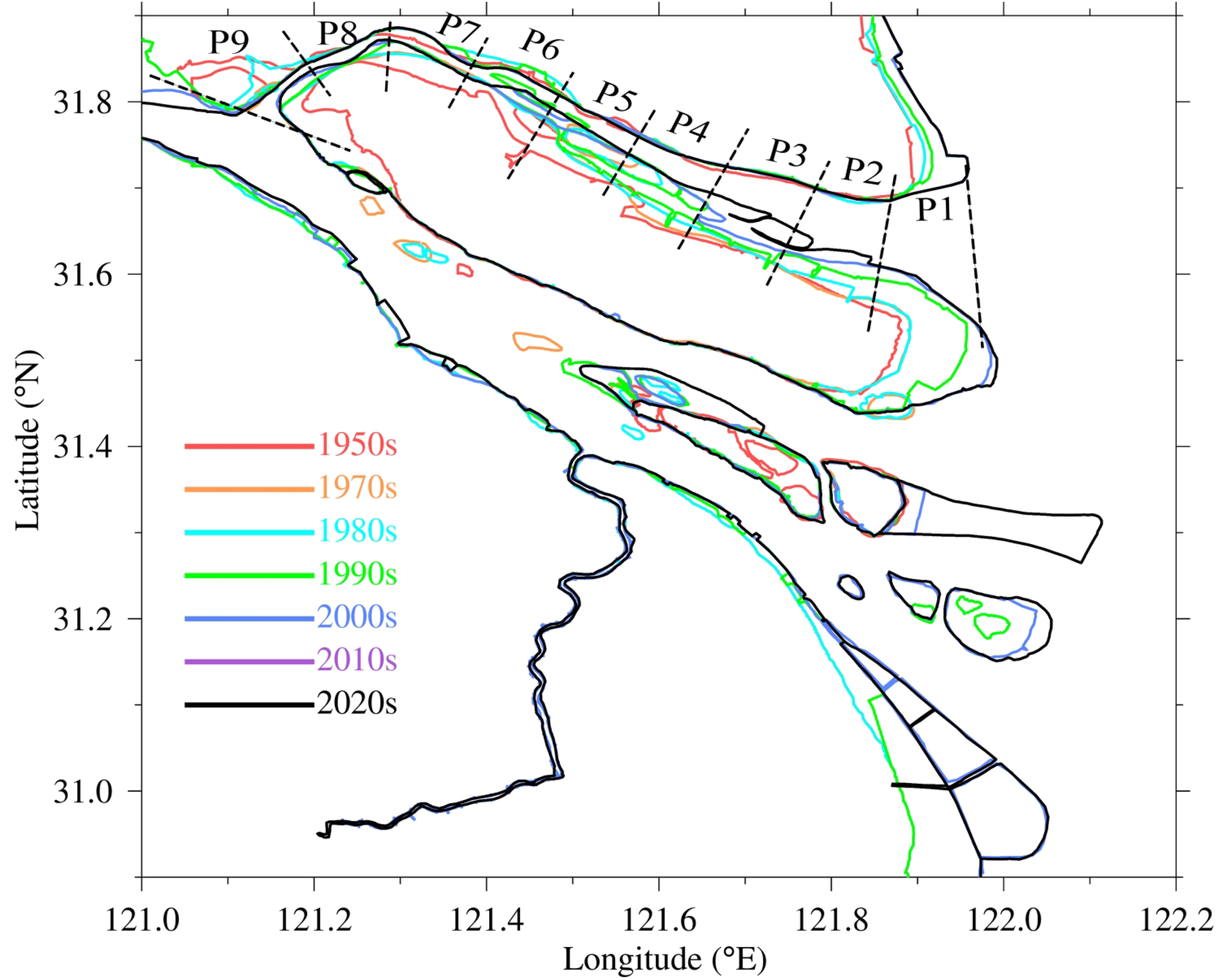
Changes in the shoreline of the Yangtze River Estuary from the 1950s to the 2020s. The NB is uniformly divided into 9 parts, P1–P9, for calculating the channel area and volume. Red line: 1950s; orange line: 1970s; cyan line: 1980s; green line: 1990s; blue line: 2000s; purple line: 2010s; and black line: 2020 (hereinafter the same).
Owing to natural evolution and human intervention, the topography of the Yangtze River Estuary underwent significant changes from the 1950s to the 2020s. The NB experienced the most drastic changes, and its area and volume persistently decreased (Table 1). From the 1950s to the 2020s, the channel area of the NB decreased from 813 million m2 to 362 million m2, a reduction of 55.56%. The channel volume decreased from 4.14 billion m3 to 1.76 billion m3, a reduction of 57.57%. The most severe decline in channel area occurred from the 1980s to the 2000s, with an average annual decrease exceeding 10 million m2. The sharpest decrease in channel volume occurred between the 1980s and 1990s, when it decreased by 661 million m3 annually. The substantial changes in the NB from the 1980s to the 2000s were primarily caused by the extensive reclamation projects being performed in Chongming East Shoal, Lingdiansha, Xinglongsha, and Xincunsha.
Table 1
| Variables | 1950s | 1970s | 1980s | 1990s | 2000s | 2010s | 2020s |
|---|---|---|---|---|---|---|---|
| Channel area (108 m²) | 8.13 | 7.45 | 6.61 | 5.52 | 4.49 | 3.87 | 3.62 |
| Channel volume (109 m³) | 4.14 | 3.41 | 3.01 | 2.35 | 2.08 | 1.93 | 1.76 |
Channel area and volume of the NB in different decades.
A more detailed depiction of changes in the channel width and cross-sectional area along the NB is analyzed. The channel is uniformly divided into 9 parts, P1 to P9 (Figure 5), from upstream to downstream. The channel width and cross-sectional area persistently decreased from the 1950s to the 2020s (Figures 6a, c).
Figure 6

Distribution (left) and variation (right) of the width (a, b), cross-sectional area (c, d) and modeled maximum tidal range (e, f) along the NB (0 km in the lower section) from the 1950s to the 2020s.
During the 1950s–1970s, channel narrowing occurred primarily in the middle–upper section, especially in P5–P8 (Figure 6b), with reductions of 31.93%, 22.41%, 37.73% and 34.81%, respectively. The cross-sectional area decreased significantly (29.26%), with the reduction being far greater downstream (26.81%) than upstream (3.96%). P1 showed the smallest decrease of 17.41%, whereas P8 showed the greatest decrease of 51.45% (Figure 6d).
During the 1970s–1980s, channel narrowing occurred mainly in the lower–middle section (P2–P4) and the upper section (P8–P9). The channel width in P2 and P4 decreased by 20.97%. The cross-sectional area decreased substantially in all parts except for the upper reach, P8–P9. The decreases ranged from a minimum of 13.07% in P8 to a maximum of 25.13% in P2.
During the 1980s–1990s, channel narrowing was concentrated in the middle and upper section, particularly P6 and P7 in the upper–middle section and P9 near the difluence of the NB and SB, with reductions of 37.64%, 30.21%, and 25.30% for P6, P7, and P9, respectively. The cross-sectional area decreased in all parts except for P1, whose average increase was small (1.74%). The greatest decreases occurred in P6, P7 and P9, reaching 37.59%, 32.05% and 37.87%, respectively.
During the 1990s–2000s, channel narrowing in the NB was particularly severe. Narrowing exceeded 10% in all parts, surpassing 30% in P3–P4 and P8–P9. P9 experienced a narrowing rate exceeding 45%. The cross-sectional area reduction was severe, especially in the middle–lower P3 and upper P8–P9, with decreases of 33.34%, 50.34% and 41.53%, respectively.
During the 2000s–2010s, the channel narrowing trend was moderate (14.84%). The degree of narrowing reached 26.38% and 31.78% in P5 and P6, respectively, but the reductions in the other parts were less than 23.06%. The cross-sectional area decreased slightly in the middle–lower section (P1–P6, -9.09%) but increased significantly in the upper section (P7–P9, 45.62%). The most severe decrease (20.95%) occurred in P2, whereas the greatest increase (64.49%) occurred in P8.
During the 2010s–2020s, significant channel narrowing occurred only in P2 (22.72%) and P8 (10.01%). The channel narrowing in the other parts was less than 4.85%. The cross-sectional area generally decreased downstream (-13.52%) but increased upstream (1.56%). Apart from a significant decrease in P2 of 24.35%, the changes in the other parts were relatively small. The greatest increase in P9 was 6.18%.
In summary, the NB has been narrowing distinctly since the 1950s and experienced moderate channel narrowing after the 2010s. The cross-sectional area of the entire NB significantly decreased before the 21st century and still decreased in the lower section but increased in the upper section of the NB after the 21st century.
3.2 Tidal prism and tide range in the north branch
The simulated elevation time series at point S1 (Figure 1) under the 1950s estuarine topography, along with the periods for the tidally averaged tidal prism, salinity, water flux and salt flux in spring–neap tide, are shown in Figure 7. From the 1950s to the 2020s, the tidal prism constantly decreased across Sec. 3 in the NB (Table 2), with a reduction exceeding 62.32% during spring–neap tide. The decline was less pronounced during spring tides (-59.58%) than during neap tides (-62.89%). The decline in the tidal prism during spring–neap tide was relatively small (-7.59%) from the 1950s to the 1970s, with a greater reduction (>18.19%) from the 1970s to the 1980s, a moderate decrease (12.85%) from the 1990s to the 2000s, and the greatest decrease (-24.48%) from the 2000s to the 2010s, with a further slow decline (~9.88%) from the 2010s to the 2020s.
Figure 7
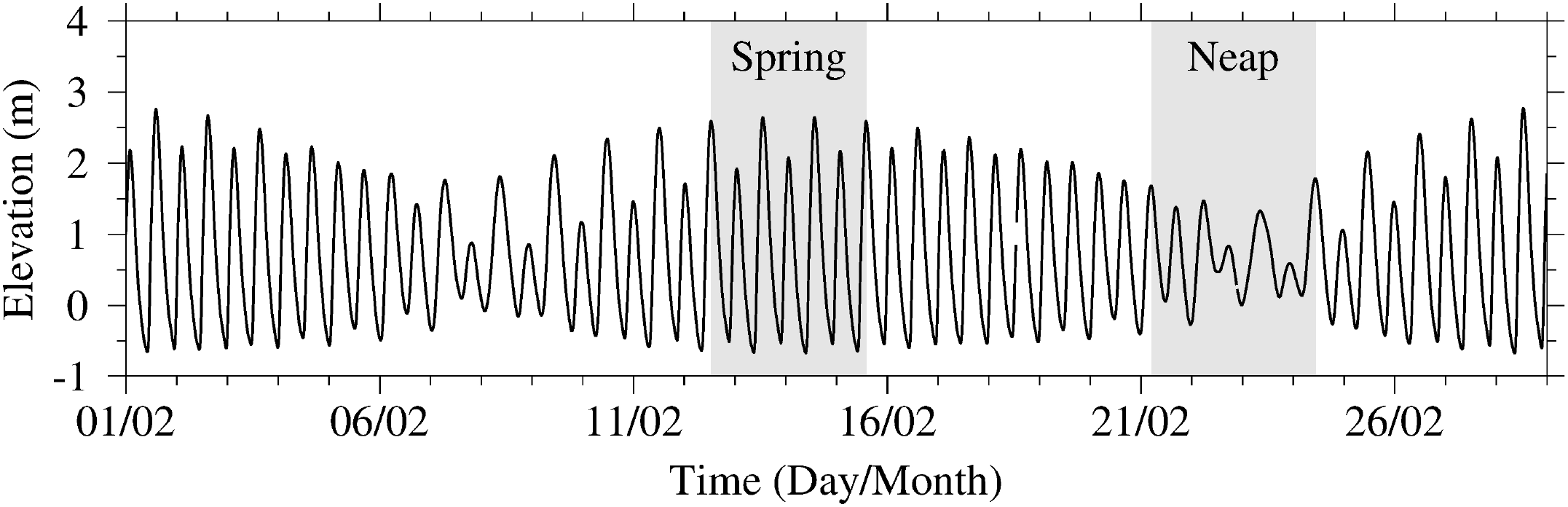
Modeled time series of elevation at point S1 under the topography of the 1950s. Gray shadows: tidally averaged periods during spring tide, MAS tide, neap tide and MAN tide.
Table 2
| Tidal type | 1950s | 1970s | 1980s | 1990s | 2000s | 2010s | 2020s |
|---|---|---|---|---|---|---|---|
| Spring-neap | 14.26 | 13.17 | 10.78 | 9.38 | 7.89 | 5.96 | 5.37 |
| Spring | 17.96 | 16.53 | 13.59 | 12.12 | 10.39 | 7.93 | 7.26 |
| Neap | 6.12 | 5.40 | 4.60 | 4.13 | 3.51 | 2.49 | 2.29 |
Tidal prism of the NB during spring–neap, spring and neap tides from the 1950s to the 2020s (unit: 108 m³).
The simulated maximum tidal range along the NB from the 1950s to the 2020s exhibited more complex variations than the tidal prism did (Figure 6e). The bottom section of the NB feature a funnel-shaped topography that gradually narrowed upstream, causing the tidal range to increase in the lower section and then decrease upstream, with the minimum tidal range occurring at the difluence of the NB and SB. In the 1950s, the maximum tidal range was 4.55 m at 29 km along the NB, and the minimum tidal range was 2.87 m. In the 1970s, the maximum tidal range increased to 4.70 m at 23 km, and the minimum tidal range was 2.80 m. Compared with those in the 1950s, the tidal ranges generally increased, except in P9; the greatest increase of 7.82% occurred in P7 (Figure 6f). In the 1980s, the maximum tidal range was 4.58 m at 18 km, and the minimum was 2.82 m. Compared with those in the 1970s, the tidal ranges generally decreased, especially in the middle section, with the greatest decline of 8.46% occurring in P7. In the 1990s, the maximum tidal range increased to 4.98 m at 17 km, and the minimum remained at 2.82 m. Compared with those in the 1980s, the tidal ranges increased in the middle and lower section but decreased in the upper section.
In the 2000s, the maximum tidal range increased to 5.04 m at 19 km, and the minimum increased to 3.09 m. Compared with those in the 1990s, the tidal ranges increased overall, particularly in upper P7, P8 and P9, which increased by 24.58%, 17.02%, and 11.86%, respectively. In the 2010s, the maximum tidal range was 4.86 m at 26 km, and the minimum tidal range was 3.45 m. Compared with those in the 2000s, the tidal ranges generally decreased by approximately 1.67% to 5.57%, except in P9 near the difluence zone, where the range increased by 12.98%. In the 2020s, the maximum tidal range was 4.67 m at 16 km, and the minimum tidal range was 3.49 m. Compared with those in the 2010s, the tidal ranges slightly decreased by 2.08% to 4.51% in the lower section (P1 to P4) and most of the upper section (P9) but slightly increased in the middle–upper section (P5–P8), with the greatest increase of 2.11% occurring in P6.
The tidal prism of the NB across Sec. 3 (Figure 1) in spring and neap tides from the 1950s to the 2020s is shown in Table 2. In spring tides, the maximum tidal prism in the NB occurred in the 1950s, with a value of 17.96×10⁸ m3 because it had the greatest channel width and area at the river mouth (Table 1), and the minimum tidal prism occurred in the 2020s, with a value of 7.26×10⁸ m3 because it had the smallest channel width and area at the river mouth. In the neap tides, the maximum tidal prism occurred in the 1950s, with a value of 6.12×10⁸ m3, and the minimum tidal prism was in the 2020s, with a value of 2.29×10⁸ m3.
3.3 Salinity intrusion in the north branch
Undoubtedly, changes in river topography significantly alter estuarine hydrodynamics and salinity intrusion patterns. For instance, studies in the Pearl River Estuary and the Weser Estuary have demonstrated that both natural processes and anthropogenic interventions have driven profound topographic transformations, leading to dramatic shifts in hydrodynamic regimes and salinity intrusion dynamics (Yuan and Zhu, 2015; Liu et al., 2019; Kolb et al., 2022). Salinity intrusion events of the Yangtze River Estuary in different decades from the 1950s to the 2020s were simulated under monthly mean wind and river discharge to investigate the evolution of WSO and SSO. In the 1950s, the NB was filled with saline water, and the SSO occurred during that decade (Figure 8a). Influenced by the SSO, water with a salinity greater than 0.45 psu (the salinity standard of drinking water) was transported along the northern shore of the SB in spring tides. In neap tides, the saltwater that transported downstream due to the persistent SSO during spring tide converged with saltwater that intruded from the North Channel, resulting in the salinity exceeding 0.45 psu along the south coast of Chongming Island (Figure 8b).
Figure 8
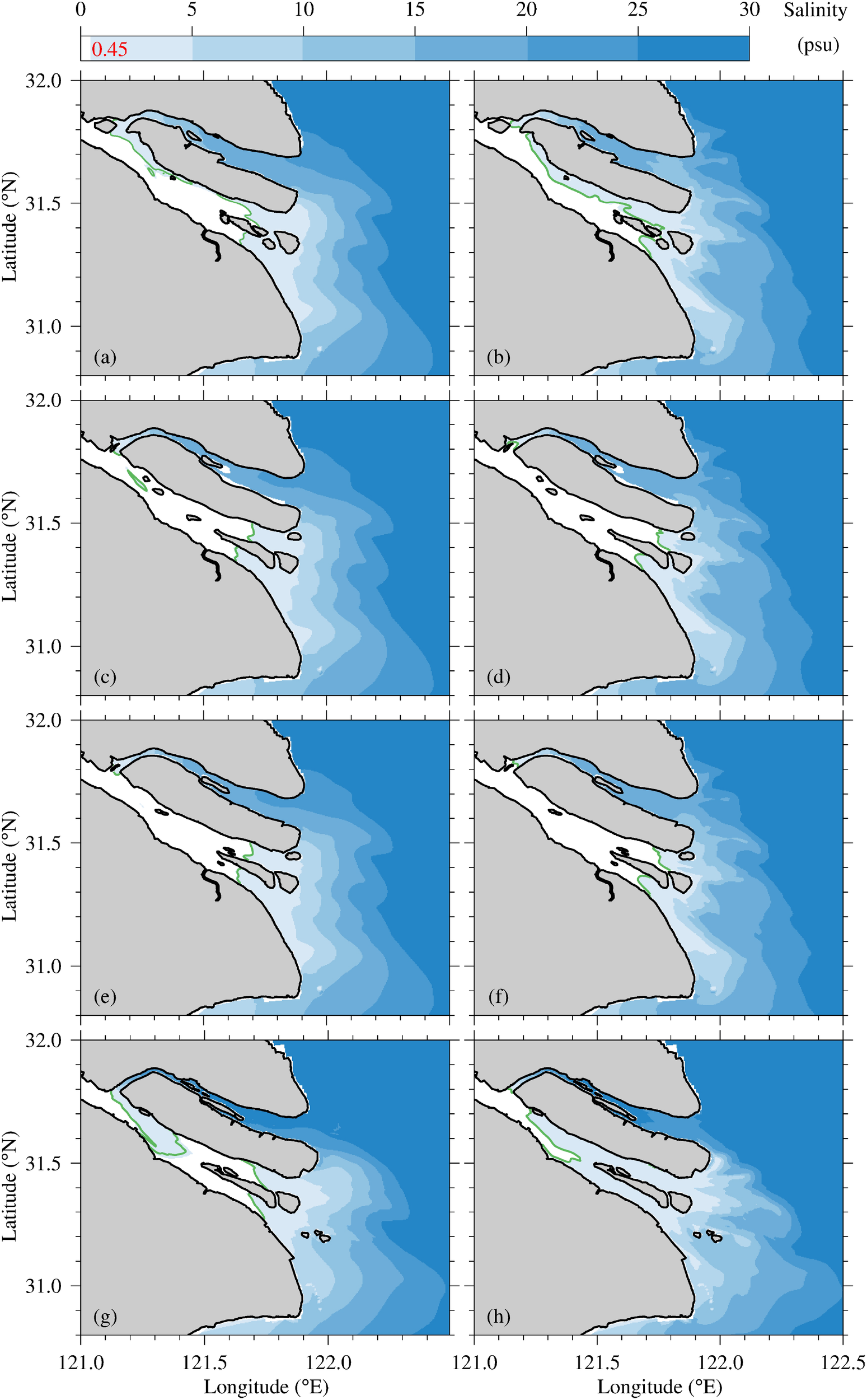
The tidal-depth-averaged salinity distributions in the 1950s (a, b), 1970s (c, d), 1980s (e, f) and 1990s (g, h). Green line: 0.45 psu isohaline, hereinafter the same. Left: spring tide; right: neap tide.
In the 1970s, the intensity of the salinity intrusion in the NB weakened. In spring tides, only a small amount of saltwater spilled into the SB, resulting in a small saltwater mass appearing in the upper section of the SB (Figure 8c). In neap tides, a small freshwater area appeared in the upper NB (Figure 8d). Compared with that in the 1950s, the SSO level dramatically weakened.
During the 1980s, the intensity of the salinity intrusion in the NB further weakened. In spring tides, the SSO disappeared, and saltwater was not present in the SB (Figure 7e). In neap tides, the area of freshwater in the upper NB increased (Figure 8f).
In the 1990s, the salinity intrusion in the NB and the SSO increased significantly. During spring tides, large amounts of saltwater spilled into the SB, causing extensive areas of saltwater to appear in the upper and middle section of the SB. The saltwater even reached the southern shore in the middle section of the SB (Figure 8g). During neap tides, the SSO disappeared. The saltwater that spilled into the SB during spring tide moved downstream and converged with the frontal intrusion saltwater in the North and South Channel. This convergence resulted in only a small area of freshwater remaining in the upper section and along the southern shore of the middle section of the SB (Figure 8h).
In the 2000s, the salinity intrusion and SSO further increased, resulting in significant decreases in the freshwater in the SB. During spring tides, substantial saltwater entered the SB from the NB, which was transported downstream and spread southward, with freshwater only being present in an area adjacent to the difluence of the North Channel and South Channel (Figure 9a). During the neap tides, SSO still existed, and saltwater was further transported downstream, converging with the frontal intrusion saltwater from the North Channel and South Channel and restricting freshwater to a small zone along the southern shore of the upper section of the SB (Figure 9b).
Figure 9
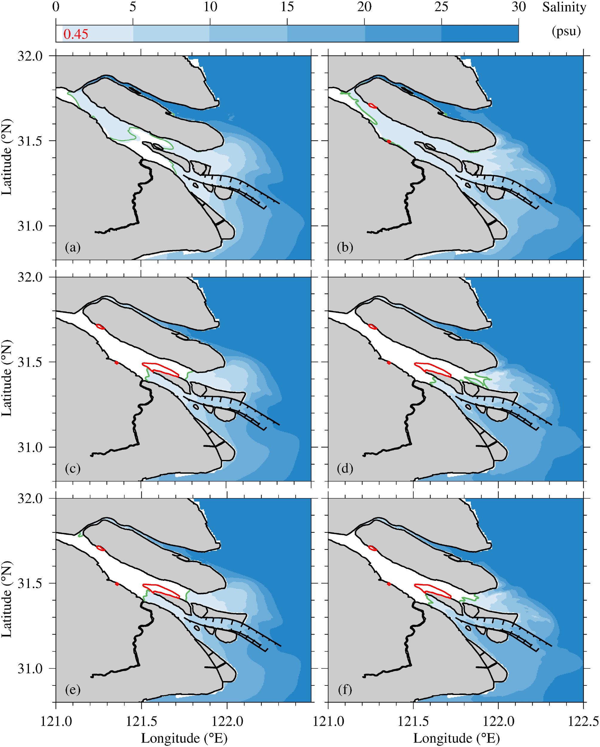
The tidal-depth-averaged salinity distributions in the 2000s (a, b), 2010s (c, d) and 2020s (e, f). Left: spring tide; right: neap tide.
In the 2010s, the salinity intrusion in the NB weakened substantially, and the SSO disappeared. Small amounts of freshwater emerged in the upper NB in both spring and neap tides (Figures 9c, d). Salinity intrusion weakened in the North Channel and increased in the South Channel compared with that in the 2000s.
By the 2020s, the salinity intrusion in the NB and the SSO intensified slightly. During spring tides, the SSO was very weak, and freshwater was present throughout the entire SB (Figure 9e). During neap tides, a small amount of freshwater persisted in the upper NB (Figure 9f).
The results of the salinity intrusion simulation showed that the evolution of the SSO experienced weakening–enhancing–weakening processes. The SSO already existed in the 1950s and weakened in the 1970s and 1980s; it distinctly increased in the 1990s, reached its most severe level in the 2000s, and significantly weakened in the 2010s and 2020s.
The positions of isohalines in the NB during different decades are shown in Figure 10. Before and during the 2000s, the 5 isohaline migrated farther upstream during flood tide of spring tides and retreated approximately 10 km during neap tides. The 10 isohaline was far from the difluence of the NB and SB, less influenced by river discharge, and more controlled by tides. This isohaline migrated farther upstream during spring tides. Compared with the 5 isohaline, the 15 isohaline in the 1950s, 1970s, 1980s, 2010s and 2020s distinctly and slightly moved downstream in the 1990s and 2000s. The 20 isohaline was in the upper section during spring tides and in the upper–middle section during neap tides, which were farther from the estuary mouth in the 1990s and 2020s. From the 1950s to the 1980s, the isohalines were located farther downstream during neap tides than during spring tides. This shift was primarily due to the influence of low-salinity water discharged from the North Channel (Figure 8) and enhanced tidal pumping during spring tides (Wu et al., 2011).
Figure 10
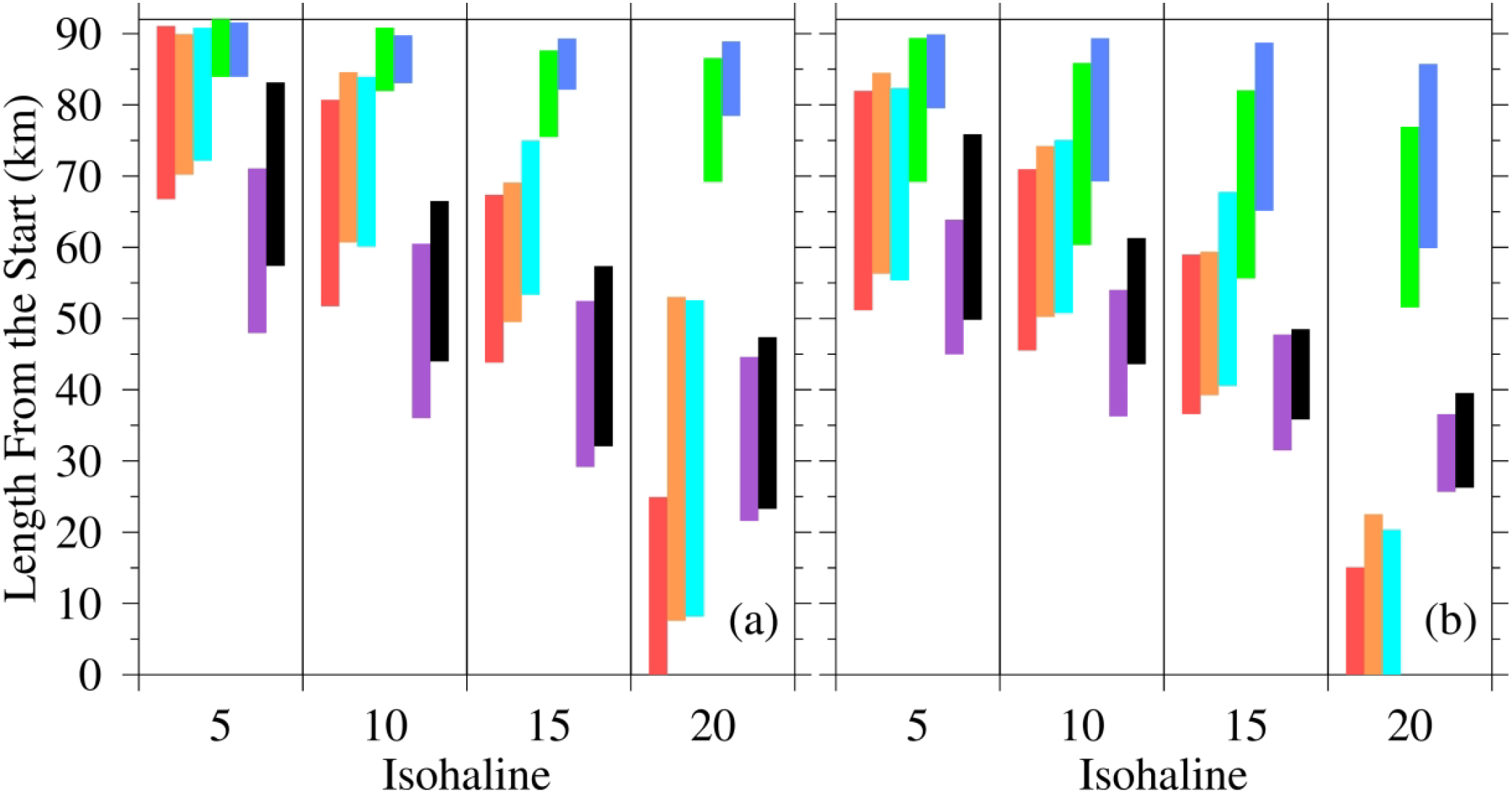
Positions of the 5, 10, 15 and 20 isohalines in the NB from the 1950s to 2020s. (a) spring tides; (b) neap tides.
The positions of isohalines indicated that there was a distinct evolution process of weakening–enhancing–weakening in terms of salinity intrusion from the 1950s to the 2020s. During the 1950s–1980s, the isohalines of 5, 10 and 15 periodically oscillated with tidal movements in the mid-to-upper section of the NB. The 20 isohaline retreated beyond the estuary mouth during ebb tides during spring tides in the 1950s and during neap tides in the 1950s, 1970s and 1980s. In the 1990s and 2000s, all isohalines moved far upstream, indicating that the salinity intrusion in the NB significantly increased. In particular, in the 2000s, the 20 isohaline reached its farthest upstream position at 88.5 and 85.2 km during spring and neap tides, respectively. In the 2010s and 2020s, the salinity intrusion in the NB weakened, and all the isohalines moved significantly downstream.
4 Discussions
Previous analyses revealed that since the 1950s, the NB has consistently been narrowing and shallowing, resulting in a continuous decrease in the tidal prism and range. However, the SSO did not consistently weaken; it decreased from the 1950s to the 1980s, significantly increased from the 1980s to the 2000s, and decreased from the 2000s to the 2020s. The SSO was related not only to the tidal prism and range but also to the tidal asymmetry, residual water flux (RWF), residual salt flux (RSF) and water diversion ratio (WDR) in the upper section of the NB. In this section, we discuss the SSO evolution from the perspectives of tidal asymmetry, RWF, RSF and WDR.
Sec. 2 is located at the bifurcation of the NB and SB, serves as a critical cross-section for monitoring both WSO and SSO. Influenced by the tidal phase difference between the two branches, its flood–ebb dynamics are notably complex. Similar to other estuarine regions, Sec. 2 exhibits pronounced tidal duration asymmetry. Except during spring tides in the 2010s, flood duration has consistently been shorter than ebb duration. Across the period from the 1950s to the 2020s, the flood–ebb duration gap (defined as ebb duration minus flood duration) displayed distinct decadal evolution. For spring–neap tides, the gap decreased from 2.41 h in the 1950s to a negative value of –0.98 h in the 2000s—indicating a temporary reversal where flood duration exceeded ebb duration—and then rebounded sharply to over 3.34 h in the 2010s and 2020s. A similar pattern was observed during spring tides: the gap narrowed from 2.72 h (1950s) to –0.86 h (2000s) before increasing again to more than 1.31 h in the 2010s and 2020s. In contrast, neap tides remained remarkably stable throughout the entire period, with a consistently small gap of approximately 1.80 hours, underscoring their relative insensitivity to long-term topographic changes compared to higher-energy tidal regimes (Table 3).
Table 3
| Variables | Period | 1950s | 1970s | 1980s | 1990s | 2000s | 2010s | 2020s |
|---|---|---|---|---|---|---|---|---|
| Duration (flood/ebb, h) |
Spring-neap | 4.99/7.40 | 4.36/8.03 | 4.69/7.69 | 4.46/7.92 | 6.18/6.20 | 4.40/7.98 | 4.52/7.86 |
| Spring | 4.78/7.50 | 3.97/8.25 | 4.42/7.83 | 4.22/8.03 | 6.56/5.69 | 3.78/8.47 | 3.97/8.28 | |
| Neap | 5.61/7.36 | 5.50/7.47 | 5.39/7.58 | 5.61/7.36 | 5.67/7.31 | 5.69/7.28 | 5.64/7.31 | |
| RWF (m³/s) |
Spring-neap | -65.89 | -21.89 | -19.09 | -155.04 | -257.42 | 128.67 | 91.01 |
| Spring | -675.71 | -449.62 | -379.44 | -466.78 | -444.79 | -60.41 | -131.78 | |
| Neap | 994.57 | 491.67 | 597.78 | 412.44 | 103.36 | 430.20 | 459.22 | |
| RSF (kg/s) |
Spring-neap | -3.31 | -2.80 | -2.21 | -5.13 | -6.87 | -0.34 | -0.59 |
| Spring | -6.24 | -3.99 | -4.79 | -10.35 | -11.82 | -0.09 | -0.46 | |
| Neap | -0.22 | -0.04 | 0.12 | -0.10 | -0.96 | 0.00 | 0.00 | |
| WDR (%) |
Spring-neap | -0.53 | -0.18 | -0.15 | -1.25 | -2.07 | 1.04 | 0.73 |
| Spring | -5.67 | -4.08 | -3.17 | -3.89 | -3.71 | -0.52 | -1.13 | |
| Neap | 8.18 | 6.01 | 4.89 | 3.35 | 0.81 | 3.29 | 3.56 |
Flood and ebb duration, RWF, RSF and WDR across Sec. 2 of the NB during February, spring tide and neap tide.
The subtidal RWF and RSF—obtained by filtering out tidal oscillations—provide a more accurate representation of the net water and salt transport across Sec. 2. The competition between river discharge and tides determined the RWF and RSF. Consequently, the RWF and RSF exhibited the same spring–neap variations as the tides.
In large tidal ranges, water was transported from the NB to the SB, whereas the opposite occurs in small tidal ranges (Figure 11a). Although the strongest WSO occurred during spring tides and subsequent middle tides in the 1950s, its average WSO remained relatively small because of the relatively high spring–neap variability and few WSO days. In contrast, persistent and intense WSO in the 2000s yielded the highest average WSO. From the 1950s to the 2000s, water transport was directed from the NB to the SB, peaking in the 2000s at 257.42 m3/s; however, the 2010s and 2020s reversed this pattern, with transport rates of 128.67 m3/s and 91.01 m3/s, respectively, from the SB to the NB. During spring tides, water consistently flowed into the SB from the NB across all decades, with the strongest RWF occurring in the 1950s, reaching -675.71 m3/s. During neap tides, water transport consistently reversed, as it flowed from the SB to the NB. In the 1950s, the maximum neap tide RWF into the NB was 994.57 m3/s, while the minimum was 103.36 m3/s in the 2000s.
Figure 11
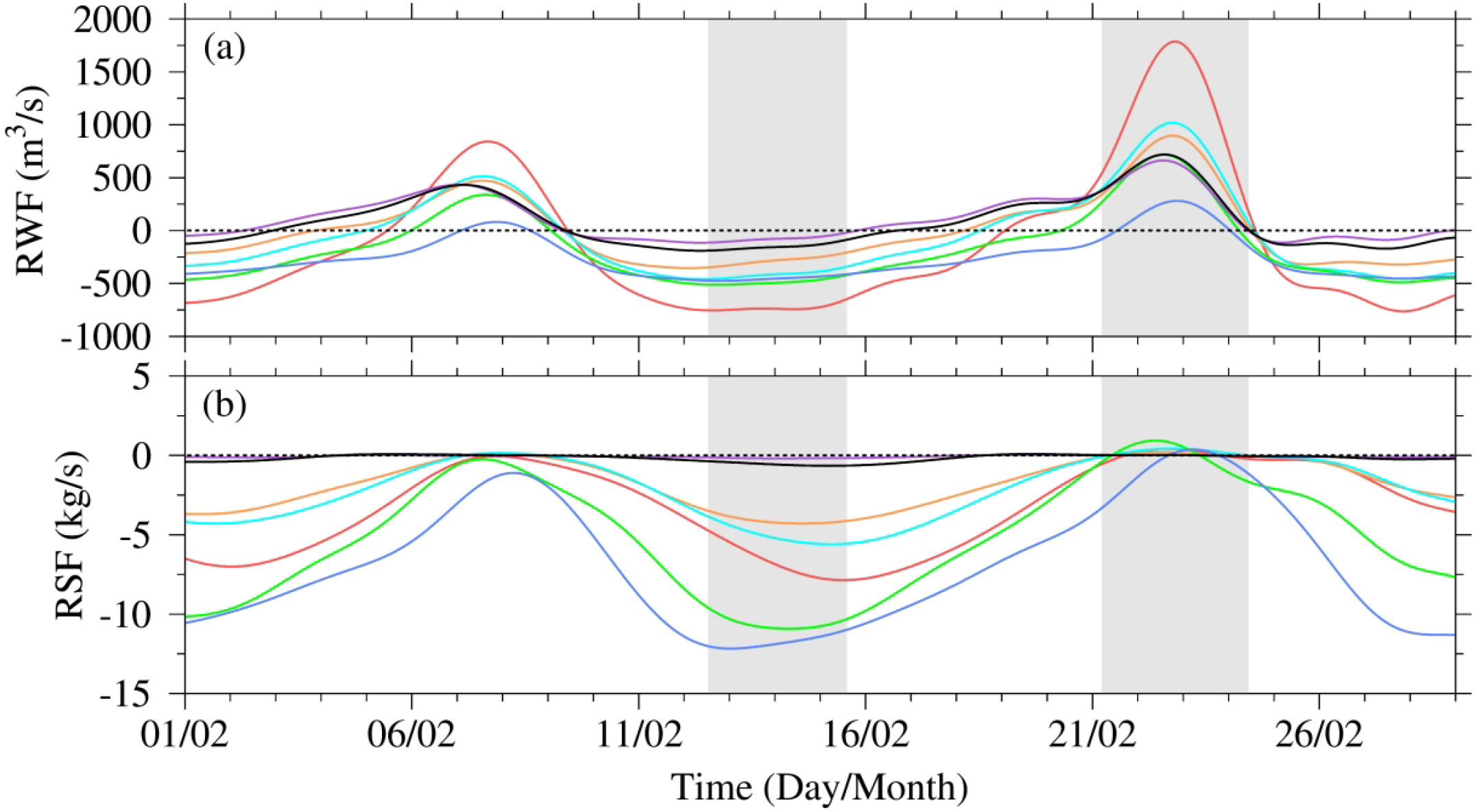
Timeseries of residual water flux (RWF) (a) and residual salt flux (RSF) (b) across Sec. 2 from the 1950s to the 2020s. Negative values represent flux from the NB into the SB. The shadow band is the spring and neap tide period.
In contrast to water transport, salt transport consistently occurred from the NB to the SB across all the decades (Figure 11b). The SSO level weakened continuously from the 1950s to the 1980s. The SSO then intensified significantly during the 1990s and 2000s, reaching approximately 6.87 kg/s in the 2000s. Subsequently, the SSO intensity decreased, with values of -0.04 and 0.19 kg/s occurring in the 2010s and 2020s, respectively. Except during neap tide, salt transport always occurred from the NB to the SB in all the decades. The intensity during spring tides was far greater than that during the two middle tides, and the middle tides after spring tide were stronger than the middle tides after neap tide. Different behaviors emerged during neap tides: salt was transported into the NB from the SB in the 1980s, while nearly no salt exchange occurred between the SB and NB in the 2010s and 2020s.
Table 3 shows the detailed values of RWF, RSF and WDR across Sec. 2 of the NB in spring and neap tides. In spring tides, the maximum WSO occurred in the 1950s, with an RWF value of 765.71 m3/s, and the minimum WSO occurred in the 2010s, with an RWF value of 0.09 m3/s. During neap tides, the RWF flowed into the NB from the SB in different decades. The maximum RWF occurred in the 1950s, with a value of 994.57 m3/s, and the minimum RWF value occurred in the 2000s, with a value of 103.36 m3/s. In February (two spring-neap circles), the RWF flowed into the SB from the NB from the 1950s to the 2000s and flowed into the NB from the SB in the 2010s and 2020s; WSO decreased from the 1950s, with a value of 65.89 m3/s, to the 1980s, with a value of 19.09 m3/s. In addition, WSO increased from the 1980s to the 2000s, and the greatest value was 257.42 m3/s. WSO vanished in the 2010s and 2020s, and the net water flux flowed into the NB from the SB, with values of 128.67 and 91.01 m3/s, respectively.
The WDR of the NB reflected how much river discharge flowed into the NB. In spring tides, the WDR was negative in all decades from the 1950s to the 2020s, indicating that the water was transported into the SB from the NB. The maximum WDR of 5.67% occurred in the 1950s, and the minimum WDR of 0.52% occurred in the 2010s. During neap tides, the WDR was positive in all decades from the 1950s to the 2020s, indicating that water was transported into the NB from the SB. The maximum WDR of 8.18% occurred in the 1950s, and the minimum WDR of 0.81% occurred in the 2010s. In February, the WDR showed the same change trend as the WDR, exhibiting the decreasing–increasing–decreasing processes of the WSO.
Unlike water transport, salt was transported into the SB from the NB during most decades and tides. During spring tides, the maximum SSO occurred in the 2000s, with an RSF value of 11.82 kg/s, and the minimum SSO occurred in the 2010s, with an RSF value of 0.09 kg/s. In the neap tides, the maximum SSO occurred in the 2000s, with an RSF value of 0.96 kg/s, and in the 1980s, salt was transported into the NB from the SB, with an RSF value of 0.12 kg/s. In the 2010s and 2020s, the RSF was 0 kg/s, and there was no SSO. Compared with that in spring tides, the RSF in neap tides dramatically decreased. In February, the RSF flowed into the SB from the NB from the 1950s to the 2020s; the SSO decreased from the 1950s, with a value of 3.31 kg/s, to the 1980s, with a value of 2.21 kg/s, and increased from the 1980s to the 2000s, with the highest value of 6.87 kg/s. The RSF was low in the 2010s and 2020s, and the net salt flux flowed into the SB from the NB, with values of 0.34 and 0.59 kg/s. From the perspectives of RWF, WDR and RSF, their change processes were consistent with the evolution of SSO.
5 Conclusions
The shoreline and water depth in different decades from the 1950s to the 2020s were collected to analyze the topography changes, and the salinity intrusion was simulated under monthly mean river discharge and wind to investigate the changes in WSO and SSO.
From the 1950s to the 2020s, the topography of the Yangtze River Estuary changed enormously, especially in the NB. Over these seventy years, the channel area of the NB decreased by 55.56%, and its channel volume decreased by 57.57%. Influenced by extensive reclamation projects, the narrowing and shallowing of the NB were the most severe between the 1980s and 2000s. After entering the 21st century, the NB tended to increase in shallowness, whereas its upper section tended to slightly deepen.
The numerical simulation results indicated that the changes in salinity intrusion and SSO in the NB experienced weakening–enhancing–weakening processes. The NB was covered by saline water and experienced SSO in the 1950s. The SSO event distinctly weakened in the 1970s and 1980s, greatly increased in the 1990s, reached its most severe level in the 2000s, and significantly weakened again in the 2010s and 2020s.
From the 1950s to the 2020s, the tidal prism of the NB constantly decreased, with a reduction of 62.32% during spring–neap tide. The decrease was less pronounced during spring tides (-59.58%) than during neap tides (-62.89%). The smallest tidal range was 4.55 m in the 1950s, and the largest tidal range was 5.04 m in the 2000s in the NB. The variations in the net water flux, net salt flux, and WDR in the upper section of the NB were consistent with the evolution processes of the SSO.
With the intensification of global climate change and anthropogenic activities, both natural and anthropogenic interventions will continue to change the estuarine topography and salinity intrusion characteristics. From the perspective of its long-term evolution, the NB will continue to become shallower, SSO would exhibit a decreasing trend. Understanding and researching the impacts of topography changes on salinity intrusion is crucial not only for enriching estuarine dynamics theory but also for ensuring the security of freshwater resources in estuarine regions.
Statements
Data availability statement
The raw data supporting the conclusions of this article will be made available by the authors, without undue reservation.
Author contributions
RM: Writing – original draft, Software, Project administration, Methodology, Conceptualization, Validation. ZZ: Writing – review & editing, Resources, Formal Analysis, Supervision, Visualization, Data curation. YY: Writing – review & editing, Investigation, Software, Validation, Data curation. ZG: Formal Analysis, Project administration, Writing – review & editing, Supervision. JZ: Funding acquisition, Conceptualization, Writing – review & editing. YW: Writing – review & editing, Formal Analysis, Resources.
Funding
The author(s) declared that financial support was received for this work and/or its publication. This work was supported by the National Natural Science Foundation of China (grant U2340225, 42276174), and the National Key R&D Program of China (grant 2022YFA1004404).
Conflict of interest
The author(s) declared that this work was conducted in the absence of any commercial or financial relationships that could be construed as a potential conflict of interest.
Generative AI statement
The author(s) declared that generative AI was not used in the creation of this manuscript.
Any alternative text (alt text) provided alongside figures in this article has been generated by Frontiers with the support of artificial intelligence and reasonable efforts have been made to ensure accuracy, including review by the authors wherever possible. If you identify any issues, please contact us.
Publisher’s note
All claims expressed in this article are solely those of the authors and do not necessarily represent those of their affiliated organizations, or those of the publisher, the editors and the reviewers. Any product that may be evaluated in this article, or claim that may be made by its manufacturer, is not guaranteed or endorsed by the publisher.
References
1
Aziz D. Tarya A. (2024). Saltwater intrusion at Kapuas Besar estuary using 1-dimensional analytical method. IOP. Conf. Series.: Earth Environ. Sci.1298, 012003. doi: 10.1088/1755-1315/1298/1/012003
2
Blumberg A. F. Mellor G. L. (1987). A description of a three-dimensional coastal ocean circulation model. Coast. Estuar. Sci.4, 1–16. doi: 10.1029/CO004p0001
3
Chen M. Xian Y. Huang Y. Sun Z. Wu C. (2024). Geographical features and development models of estuarine cities. J. Geogr. Sci.34, 25–40. doi: 10.1007/s11442-024-2193-3
4
Chen Q. Zhu J. Lyu H. Pan S. Chen S. (2019). Impacts of topography change on saltwater intrusion over the past decade in the Changjiang estuary, Estuarine. Coast. Shelf. Sci.231, 106469. doi: 10.1016/j.ecss.2019.106469
5
Delgado A. L. Menéndez M. C. Piccolo M. C. Perillo G. M. E. (2017). Hydrography of the inner continental shelf along the southwest Buenos Aires province, Argentina: influence of an estuarine plume on coastal waters. J. Coast. Res.33, 907–916. doi: 10.2112/JCOASTRES-D-16-00064.1
6
Ge J. Lu J. Ding L. P. (2022). Saltwater intrusion-induced flow reversal in the Changjiang estuary. J. Geophys. Res.: Ocean.127, e2021JC018209. doi: 10.1029/2021JC018270
7
Guo W. Jiao X. Zhou H. Zhu Y. Wang H. (2022). Hydrologic regime alteration and influence factors in the Jialing River of the Yangtze River, China. Sci. Rep.12, 11166. doi: 10.1038/s41598-022-15127-4
8
Hlaing N. O. Azhikodan G. Yokoyama K. (2024). Effect of monsoonal rainfall and tides on salinity intrusion and mixing dynamics in a macrotidal estuary. Mar. Environ. Res.202, 106791. doi: 10.1016/j.marenvres.2024.106791
9
Jumain M. Ibrahim Z. Makhtar M. Ishak R. Mohamed Rusli N. Mat Salleh M. Z. (2022). Spatio-temporal patterns of saltwater intrusion in a narrow meandering channel. Int. J. Integr. Eng.14, 188–194. doi: 10.30880/ijie.2022.14.09.024
10
Jung N. W. Lee G. H. Dellapenna T. M. Jung Y. Jo T. C. Chang J. et al . (2024). Economic development drives massive global estuarine loss in the Anthropocene. Earth’s. Future12, e2023EF003691. doi: 10.1029/2023EF003691
11
Kolb P. Zorndt A. Burchard H. Gräwe U. Kösters F. (2022). Modelling the impact of anthropogenic measures on saltwater intrusion in the Weser estuary. Ocean. Sci.18, 1725–1739. doi: 10.5194/os-18-1725-2022
12
Kwak D. H. Song Y. S. Choi Y. H. Kim K. M. Jeong Y. H. (2023). Influence of sluice gate operation on salinity stratification and hypoxia development in a brackish estuary dam. Reg. Stud. Mar. Sci.57, 102731. doi: 10.1016/j.rsma.2022.102731
13
Li D. Liu B. Lu Y. Fu J. (2024). The characteristic of compound drought and saltwater intrusion events in the several major river estuaries worldwide. J. Environ. Manage.350, 119659. doi: 10.1016/j.jenvman.2023.119659
14
Liu B. Peng S. Liao Y. Wang H. (2019). The characteristics and causes of increasingly severe saltwater intrusion in Pearl River Estuary, Estuarine. Coast. Shelf. Sci.220, 54–63. doi: 10.1016/j.ecss.2019.02.041
15
Lyu H. Zhu J. (2018). Impact of the bottom drag coefficient on saltwater intrusion in the extremely shallow estuary. J. Hydrol.557, 838–850. doi: 10.1016/j.jhydrol.2018.01.010
16
Ma R. Qiu C. Zhu J. Zhang Z. Zhu Y. Kong L. et al . (2025). Dynamic cause of saltwater intrusion extremes and freshwater challenges in the Changjiang estuary in flood season of 2022. Front. Mar. Sci.12, 00000. doi: 10.3389/fmars.2025.1573883
17
Ma R. Zhu J. (2022). Water and salt transports in the Hengsha Channel of Changjiang Estuary. J. Mar. Sci. Eng.10, 72. doi: 10.3390/jmse10010072
18
Mekonnen M. M. Hoekstra A. Y. (2016). Sustainability: four billion people facing severe water scarcity. Sci. Adv.2, e1500323. doi: 10.1126/sciadv.1500323
19
Murphy A. H. (1988). Skill scores based on the mean square error and their relationships to the correlation coefficient. Mon. Weather. Rev.116, 2417–2424. doi: 10.1175/1520-0493(1988)116<2417:SSBOTM>2.0.CO;2
20
Pritchard D. W. (1952). Salinity distribution and circulation in the Chesapeake Bay estuarine system. J. Mar. Res.23, 11–106.
21
Scroccaro I. Spitz Y. H. Seaton C. M. (2023). Effect of local winds on salinity intrusion in the Columbia River estuary. Water15, 326. doi: 10.3390/w15020326
22
Shen H. Mao Z. Zhu J. (2003). “ Saltwater intrusion in the Changjiang estuary,” in Saltwater intrusion in the changjiang estuary ( China Ocean Press, Beijing).
23
Tao Z. Chen Y. Pan S. Chu A. Xu C. Yao P. et al . (2024). The influence of wind and waves on saltwater intrusion in the Yangtze estuary: a numerical modeling study. J. Geophys. Res.: Ocean.129, e2024JC021076. doi: 10.1029/2024JC021076
24
Wang N. Ge J. (2025). Predictions of saltwater intrusion in the Changjiang estuary: integrating machine learning methods with FVCOM. J. Hydrol.653, 132739. doi: 10.1016/j.jhydrol.2025.132739
25
Wu H. Zhu J. (2010). Advection scheme with 3rd high-order spatial interpolation at the middle temporal level and its application to saltwater intrusion in the Changjiang estuary. Ocean. Model.33, 33–51. doi: 10.1016/j.ocemod.2009.12.001
26
Wu T. Zhu J. Ma R. Qiu W. Yuan R. (2023). Freshwater resources around the reclaimed new land on the eastern Hengsha Shoal in the Changjiang estuary. Front. Mar. Sci.10. doi: 10.3389/fmars.2023.1302091
27
Wu H. Zhu J. Shen J. Wang H. (2011). Tidal modulation on the Changjiang river plume in summer. J. Geophys. Res.: Ocean.116, C00J02. doi: 10.1029/2011JC007209
28
Yang Y. Zhu J. Chen Z. Ma R. (2023). The impact of sluice construction in the north branch of the Changjiang estuary on saltwater intrusion and freshwater resources. J. Mar. Sci. Eng.11, 2107. doi: 10.3390/jmse11112107
29
Yuan R. Zhu J. (2015). The effects of dredging on tidal range and saltwater intrusion in the pearl river estuary. J. Coast. Res.31, 1357–1362. doi: 10.2112/JCOASTRES-D-14-00224.1
30
Zhang J. Cheng L. Wang Y. Jiang C. (2023). The impact of tidal straining and advection on the stratification in a partially mixed estuary. Water15, 339. doi: 10.3390/w15020339
31
Zhang E. Savenije H. H. G. Wu H. Kong Y. Zhu J. (2011). Analytical solution for salt intrusion in the Yangtze estuary, China, Estuarine. Coast. Shelf. Sci.91, 492–501. doi: 10.1016/j.ecss.2010.11.008
32
Zhu J. Cheng X. Li L. Lyu H. (2020). Dynamic mechanism of an extremely severe saltwater intrusion in the Changjiang estuary in February 2014. Hydrol. Earth Syst. Sci.24, 3023–3036. doi: 10.5194/hess-24-5043-2020
Summary
Keywords
estuarine reservoir, multi-branching estuaries, salinity intrusion, salt-spilling-over, topography changes
Citation
Ma R, Zhang Z, Yang Y, Guo Z, Zhu J and Wang Y (2026) Influences of topography changes on the evolution of salinity intrusion in the North Branch of the Yangtze River Estuary over the past 70 years. Front. Mar. Sci. 13:1765269. doi: 10.3389/fmars.2026.1765269
Received
11 December 2025
Revised
05 January 2026
Accepted
13 January 2026
Published
30 January 2026
Volume
13 - 2026
Edited by
Toru Miyama, Japan Agency for Marine-Earth Science and Technology, Japan
Reviewed by
Jian Zhou, Hohai University, China
Xiaomei Ji, Hohai University, China
Updates
Copyright
© 2026 Ma, Zhang, Yang, Guo, Zhu and Wang.
This is an open-access article distributed under the terms of the Creative Commons Attribution License (CC BY). The use, distribution or reproduction in other forums is permitted, provided the original author(s) and the copyright owner(s) are credited and that the original publication in this journal is cited, in accordance with accepted academic practice. No use, distribution or reproduction is permitted which does not comply with these terms.
*Correspondence: Jianrong Zhu, jrzhu@sklec.ecnu.edu.cn
Disclaimer
All claims expressed in this article are solely those of the authors and do not necessarily represent those of their affiliated organizations, or those of the publisher, the editors and the reviewers. Any product that may be evaluated in this article or claim that may be made by its manufacturer is not guaranteed or endorsed by the publisher.