Abstract
Blooms of the toxigenic dinoflagellate Karenia brevis are an almost annual occurrence in the eastern Gulf of Mexico, typically initiating in late summer and early fall months and terminating in late spring or earlier. The question of whether blooms have been expanding in frequency or duration has long been debated. Recently, a Bloom Severity Index (BSI) was developed that captures changes in bloom magnitude based on cell concentrations normalized to maximum observed values. Here, changes in the BSI (severity and bloom duration) were examined for the period from 1970-2019, a period of rapid climate change and increased anthropogenic pressures. This time period encompassed several changes in the Oceanic Niño Index (the El Niño-Southern Oscillation), including a shift from a highly positive to a negative North Atlantic Oscillation in the mid 1990s, bringing with it increased precipitation and more intensive storms. Annual BSI and bloom duration have increased with increasing temperatures, and blooms have also become longer in duration in relation to increased temperatures and river flows since the mid 1990s. As increased precipitation is related to increased nutrient runoff, regional fertilizer use and the anthropogenic nitrogen (N) footprint based on population census data as proxies of nitrogen loads were examined. The duration of severe blooms was highly correlated with the increasing anthropogenic N footprint, especially when BSI values were averaged across multiple years. These relationships highlight the importance of climate changes and of increasing population since the 1980s and help to explain why earlier analyses of nutrient loads and bloom severity were inconclusive. To reduce bloom severity or duration in the future, reductions in N loads and releases from the Caloosahatchee River are needed more than ever to counteract the increasing pressures from climate change.
1 Introduction
Karenia brevis is a toxigenic dinoflagellate that commonly occurs in the eastern Gulf of Mexico (Gulf of America). Typically a late summer – early fall phenomenon, blooms of this microalga have been expanding in severity and duration (Stumpf et al., 2022; Glibert et al., 2025). Blooms generally initiate towards the end of the rainy season, which occurs from mid-May to mid-October. Such events are thought to initiate in oligotrophic, offshore water, approximately 18–24 km from the coast (Steidinger, 1975; Tester and Steidinger, 1997), in association with the nitrogen (N)-fixing cyanobacterium, Trichodesmium spp (Walsh and Steidinger, 2001; O’Neil et al., 2024). The vertically stratified waters allow the K. brevis cells to persist at the base of the oligotrophic water lens, serving as inocula for near shore blooms. As the season progresses, changing wind patterns and increased upwelling transport cells into shore (Walsh et al., 2003; Liu and Weisberg, 2012) where they can thrive in a temperature niche that has been characterized as 22-28°C (Vargo, 2009; Steidinger, 2009). The Gulf of Mexico Loop Current also plays a role in upwelling, particularly when the Loop Current impinges upon the shelf slope in the southwest region of the West Florida Shelf bringing along nutrient rich deep water and accelerating water motion along the shelf (Liu et al., 2016).
Although blooms of K. brevis are an almost annual occurrence, typically terminating in spring or earlier (Heil et al., 2022), exceptionally long lasting blooms, lasting more than 10 months, can persist over the summer even when temperatures are seemingly above the optimum for growth (Magaña and Villareal, 2006; Vargo, 2009; Steidinger, 2009). Although such extended blooms are unusual, they have occurred recently in the years 2018-2019, 2020-2021, and 2022-2023 (Figure 1).
Figure 1

Distribution of Karenia brevis on the West Florida Shelf from October 2020 to September 2021. Hurricanes Eta (Nov 2020) and Elsa (June 2021) are also shown on the maps. This time series represents one of the recent prolonged blooms that spanned the summer months. Maps reproduced from FWRI (https://www.flickr.com/photos/myfwc/sets/72157635398013168/) under a creative commons license. Right panel map shows the region of Southwest Florida included in the Bloom Severity Index (BSI) as defined by Stumpf et al. (2022), reproduced under a creative commons license.
The question of whether blooms of K. brevis have been expanding in frequency, duration or severity has been debated for years, and if so, the reasons for such expansion. Blooms of this dinoflagellate have been documented since early explorers of the Florida coast (Steidinger, 2009), leading many to suggest that these events are simply natural occurrences and that anthropogenic impacts play little role, if any, in the timing or intensity of blooms. In support of latter notion, Walsh et al. (2006) did not find significant correlations between bloom occurrences and nutrient loading. They showed that while there were anthropogenic increases in phosphate from 1966-1985, as well as reductions in nitrogen (N) and phosphorus (P) loading to Lake Okeechobee, such blooms regularly persisted. Using a similar approach, Vargo et al. (2004, 2008) evaluated nutrient sources for support of blooms after initiation and transport into coastal waters and estimated that estuarine fluxes of N and P from Tampa Bay, Charlotte Harbor, and the Caloosahatchee River were sufficient to only support a moderate K. brevis bloom (3 × 10⁵ cells L−1) but would not support larger blooms. In contrast to these conclusions, Brand and Compton (2007) examined the available data on K. brevis abundance from 1954 to 2002 and reported that abundances were 13-18-fold higher in 1994–2002 compared with 1954-1963. They hypothesized that climate change may be one factor but had insufficient data to test that hypothesis. They also suggested that inshore blooms were becoming more intense due to nutrient pollution, a result due to Florida’s expanding population, which would lead to more sewage, land use and other changes, but were also unable to test those changes directly. That study, however, was criticized due to the irregularity of available bloom data (Haverkamp et al., 2004; Heil and Steidinger, 2009), leading to complexities in statistical analyses and thus uncertainties in Brand and Compton (2007) conclusions. These collective debates led Anderson et al. (2008) to suggest that conclusions regarding a link between K. brevis and eutrophication and other anthropogenic pressures were premature and that such links may be at least partially due to increased monitoring efforts, increases that began in the 1990s. Anderson et al. (2021) furthered the notion that bloom intensities have not changed based on an examination of the frequency of neurotoxic shellfish toxins (NSTs, or brevetoxins, the K. brevis dominant toxin), as reported in the international database, HAEDAT (Harmful Algal Event Data Base) from four regions in the Gulf of Mexico: the western Gulf of Mexico (Texas), the northern Gulf (Louisiana, Mississippi, and Alabama), Florida’s Gulf Coast, and Florida’s Atlantic Coast. From this database, 58 events were recorded over 30 years, and no significant trend was apparent.
Relationships between expanding human activity, actively managed discharges from the major freshwater source, the Caloosahatchee River, and K. brevis frequency have also been previously explored. In an early study, Dixon and Steidinger (2002) showed a lagged correlation between K. brevis and rainfall and river flow. Li et al. (2021) demonstrated that the probability of K. brevis blooms (defined as cell densities >105 cells L-1) increased with increasing river flows across all discharge levels and suggested that the composition of nutrients discharged by different rivers impacts localized coastal K. brevis blooms. Medina et al. (2020) applied a novel nonlinear time series approach to examine terrestrially sourced inputs of N, P, and freshwater between 2012 and 2018 and their finding supported the hypothesis that anthropogenic N runoff from the Caloosahatchee River was strongly associated with the growth of blooms (based on cell densities). That study was followed by Medina et al. (2022), who applied causal analysis methods based on chaos theory, and further showed that discharges from the Caloosahatchee River intensified blooms. Tomasko et al. (2024) recently provided evidence that from 2007-2023, total N loads from the Caloosahatchee (but not from the Myakka or Peace) Rivers correlated with bloom duration.
Sobrinho et al. (2022) examined the bloom time series from 1998–2020 and the relationships between K. brevis abundance and the El Niño–Southern Oscillation (ENSO) and its rate of change, as well as temperature, precipitation, river flow, and salinity. They confirmed that El Niño brings wet and cool weather to South Florida, including a greater frequency of storms, while La Niña brings dry and warm weather. However, mild La Niña and periods of ENSO transitions bring a higher frequency of hurricanes that directly impact Florida. Using cross-correlation of log-transformed K. brevis abundance and environmental variables with lags from 0–12 months, Sobrinho et al. (2022) found that the largest blooms occurred during transition periods in the ENSO index.
To counter the frequent critique that long term analyses of bloom events are compromised due to the irregularity of monitoring and thus of documented bloom occurrences, Stumpf et al. (2022) used historical cell count data from 1953 to 2019 (available through Florida Fish and Wildlife Research Institute, Supplementary Table 1) to develop a normalized monthly and annual Bloom Severity Index (BSI). This index was recently updated through 2023 (Li et al., 2025). The BSI includes cell count observations binned by 0.2 latitudinal degrees covering 25 km of the coast, specifically the southwest region within 5 km of the coast (25.4°-28.4°N, 82.5°-83.0°W; Figure 1), not including estuarine sites. Each bin was assigned a maximal cell concentration for each month, applying an average of values of adjacent bins if data were missing. These cell concentrations were further categorized into five levels as: <5,000 cells L-1, >5,000 cells L-1, > 50,000 cells L-1, >100,000 cells L-1, or >1,000,000 cells L-1. Once maximal concentrations for each bin were tallied, values were normalized by the highest number of bins in any given year (out of a possible 216 bins) exceeding 5000 cells L-1 and then multiplying by 10 to yield the BSI. The BSI scores severity on a scale from 0 (<5,000 cells L-1) to 10 (the maximum extent of coastline impacts by a bloom for any month during the time series assessed thus far). Different BSI values were determined for each cell threshold level. While the first two cell concentration levels represent conditions generally considered to have little or no human health risk, shellfish beds can become toxic at 5,000 cells L-1 and are required to close (Heil, 2009). Cells >100,000 L-1 represent significant blooms which can be detected by satellites, cause fish kills, and may be related to human respiratory stress, and therefore this BSI category was applied herein. The BSI provides value over direct cell abundance data because it integrates spatial extent, duration, and cell concentrations, an important consideration given the patchy nature of blooms and corresponding irregular sampling in time and space. While Stumpf et al. (2022) applied their approach to determine relationships with the reported respiratory irritation over time, they emphasized that their approach would be useful in evaluating the effects of land-based nutrient fluxes on the magnitude of K. brevis blooms. This is the approach taken herein.
In all, the different studies outlined above have used different time periods for analysis and different analytical approaches and have therefore come to somewhat different, and even conflicting, conclusions. In this study, a new look at the long-term trends in BSI relative to several climate factors, global and regional, and anthropogenic N pollution was undertaken. This approach extends the analysis of Brand and Compton (2007) with respect to impacts of climate change and Florida’s burgeoning population and applies Stumpf et al. (2022) rigorously developed BSI to test the hypothesis that increases in duration and severity have indeed occurred over the past 50 years due to changes in climate (including temperature, river flow changes and extreme events) and in anthropogenic nutrient inputs.
2 Methods
2.1 Data sources
Data from numerous publicly available data bases were used to address relationships between bloom occurrence, severity, and duration and climate indices and regional changes and anthropogenic N input (Supplementary Table 1).
Although the BSI values reported by Stumpf et al. (2022) begin from the early 1950s, the analysis herein covers only 1970-2019. This time period was chosen because it represents a substantially long period during which trends should be apparent (49 years) and because virtually all ancillary data examined herein encompassed this full period. This time period also encompasses an approximate equal number of years before and after the increase in bloom monitoring that occurred in the mid 1990s. Here, BSI data for blooms >100,000 cells L-1 were used, as this bloom density is representative of major blooms (Heil and Steidinger, 2009). These data were averaged by month and year and again by multiple years. Bloom duration was determined by summing the number of months with a positive BSI.
2.2 Changes in the Oceanic Nino Index and other physical factors: overview
To confirm whether there were climatic change points over the near-50 years examined, changes in the Oceanic Niño Index (ONI; the 3-month running averages of the El Niño-Southern Oscillation) were examined (Supplementary Table 1). When ONI is positive, El Niño activity is suggested, which normally leads to reduced rainfall and hurricane activity in the Gulf of Mexico. When ONI is negative, there are typically stronger storms in Florida, including more extreme storms and hurricanes (Gray, 1984; Bell and Chelliah, 2006). To explore this, two measures of precipitation were explored. First, regional hurricane precipitation data were downloaded (Supplementary Table 1; Supplementary Figure 1). These data reflect the precipitation patterns only for hurricanes that specifically resulted in large rainfall events along the west coast of Florida. Also, annual precipitation data were also obtained for the counties of the region, including Charlotte County, Hendee, DeSoto, Polk, Glades, Lee and Hendry counties (Supplementary Table 1). The anomalies of these regional data were calculated relative to the mean of 1970-2019.
Monthly temperature anomalies (e.g., monthly average minus the long-term (1910-2000) monthly mean) were obtained for the Gulf of Mexico (Supplementary Table 1). As changes in temperature of the Gulf of Mexico may not be representative of changes on the coastal West Florida Shelf, monthly water temperature data from Sarasota (Supplementary Table 1) were compared. Averaging the 15-year Sarasota data annually and comparing to the Gulf of Mexico record, a significant relationship was found (r=0.30, df=14, p < 0.05) and thus the longer Gulf of Mexico temperature anomaly record was deemed an appropriate metric for temperature change in the studied region.
Monthly mean Caloosahatchee River flow data were downloaded from the US Geological Survey (USGS) monitoring site at the Franklin Lock and Dam (Site S79). Annual averages as well as averages of the months with the highest flows (July through December) were calculated, as well as anomalies relative to the mean of 1970-2019.
Long term, consistent records of salinity are not available. The Florida Fish and Wildlife Research Institute database (www.myfwc.com) was queried for all K. brevis and Trichodesmium records for the studied region from 1970 to 2019. Excluding all estuarine data points, salinity averaged 35.47, with a minimum of 32.98 and a maximum of 40.00 with no consistent trend. As these values all fall within the known optimal salinity range for K. brevis (Brown et al., 2006), no further analysis of salinity trends were undertaken.
2.3 Fertilizer use, population growth and the regional nitrogen footprint
Comprehensive and consistent nutrient data are lacking for the full time course examined here. To estimate nutrient changes, two proxies were used: fertilizer use and population trends. Trends in fertilizer use by county were obtained from Falcone (2021); Supplementary Table 1). The sum of farm and nonfarm fertilizer use annually was calculated.
The population census values for the counties of the Caloosahatchee River, Peace River, and Tampa Bay watersheds were obtained for the years 1970-2019 (Supplementary Table 1). Charlotte County straddles the watersheds of the Caloosahatchee River and that of the Peace River, and the simple assumption that half of the population resides in each watershed was applied. Population census data are decadal, and interpolations were made to estimate yearly population change. Tourism data (numbers and durations of visits) are not available by county and are not included in the calculations herein.
The N footprint of the population of the watersheds of the Caloosahatchee and Peace Rivers was calculated based on the Leach et al. (2012) N-calculator tool as reported by Galloway et al. (2014). The value, 39 kg N capita-1 yr-1, is a national average for the U.S. based on the composite impact of food use and energy related items (such as housing, transportation, goods and services; Supplementary Table 2). The assumption was made that Floridians have the same N footprint as the average U.S. population. The N-footprint was calculated by year and also as a cumulative value for 5-year intervals.
2.4 Statistical approaches
A cumulative sum (CUSUM; e.g., Page, 1954, MacNally and Hart, 1997, Manly and Mackenzie, 2003; Mesnil and Petitgas, 2009) chart was used to assess periods of change in the ONI. CUSUM charts provide a robust method to assess regime shifts by filtering the high-frequency noise and smoothing the data. Following Briceño and Boyer (2010), CUSUM values were based on z-scores, and to calculate CUSUM, running sums of z-scores were calculated. Downward segments of the time series are indicative of values drifting below the long-term mean, while upward trends are indicative of values trending above the long-term mean. Here, the long-term mean was the period from 1970-2019. These analyses identified break points in ONI in 1982, 1995, and 2014. Although a change point was identified in 1982, the BSI data prior to this date are comparatively sparse, so the data have been binned into the time periods of 1970-1994, 1995-2019, and 2014-2019 (for all data that are available).
Annual trends in temperature anomalies, precipitation of regional counties of southwest Florida, and Caloosahatchee River flow were determined for the three time periods of interest, 1970-1994, 1995-2019, and 2014-2019. Relationships between bloom severity and duration and temperature, precipitation and river flow were determined using Pearson correlations. Correlations were calculated separately for the time periods before and after the major change in climate conditions in 1995. Where comparisons are drawn between mean parameters for the different time periods, ANOVA was used. Significance was set at α=0.05, 0.01 and 0.001.
The relationship between number of bloom months and total N footprint by year and by half decade periods were also related using Pearson correlations.
3 Results
3.1 Changes in the Oceanic Nino Index and other physical factors
From 1970 to the mid 1980s, the ONI was largely neutral, based on the z-CUSUM trends (Figure 2). From the mid 1980s to the mid 1990s, ONI was above the long-term mean (the mean of all years 1970-2019). Then, from the mid 1990s to the early 2010s, ONI was negative before turning positive again around 2014. The clear change point in 1995 (Figures 2a, b) was consistent with previous analyses (Briceño and Boyer, 2010) and documented changes in the North Atlantic Oscillation (Hurrel, 1995). Mean ONI values for each major time period were significantly different (1982–1994 vs 1995–2013 comparison, p <.001, df=380; 1995–2013 vs 2014–2019 comparison, p = .024, df=296).
Figure 2
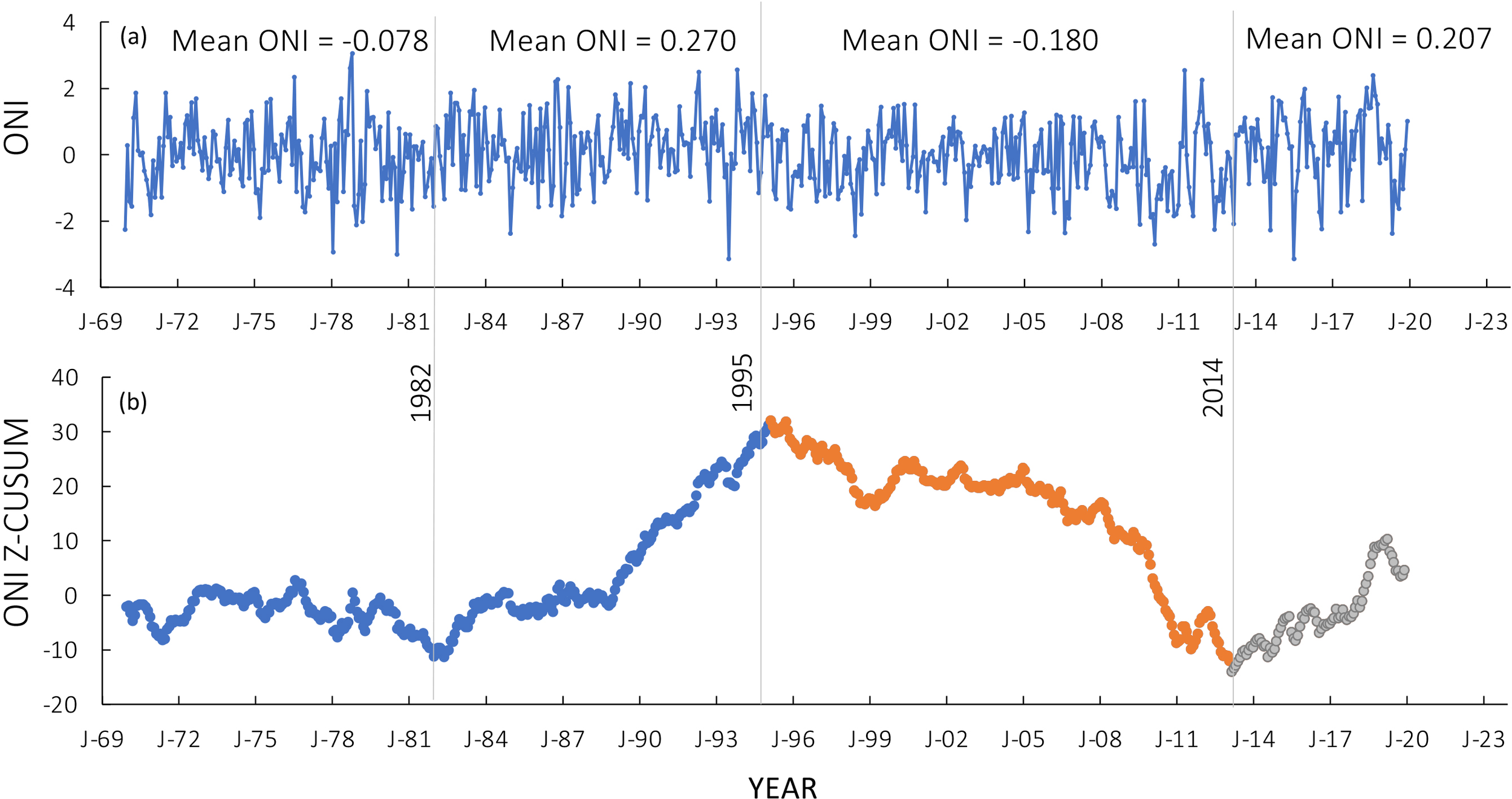
(a) Change in the Oceanic Niño Index (ONI) as a function of time (1970-2019). Mean ONI values are shown for each major time period. (b) z CUSUM trends in the ONI. Note the change points in 1982, 1995, and 2014. The shift in 1995 represented a change from a highly positive North Atlantic Oscillation phase to a more negative period and that in 2014 a reversal to a more positive phase. Data prior to the change point in 1995 are represented in blue in (b), data from 1995 to the next change point in 2014 are represented in orange, and data after 2014 are represented in gray.
In the first half of this time series (1970-1994), monthly temperature anomalies relative to the long-term monthly means were minimal (Figure 3a). However, since 1995, average monthly temperature anomalies have increased substantially, exceeding 0.2°C during virtually every year. The annual average differences between the years 1970–1994 and 1995–2019 were significant (mean 1970-1994 = -0.0161, mean 1995-2019 = 0.336; p=<.001, df =48). In the most recent years, since 2014, temperature anomalies averaged 0.66°C.
Figure 3
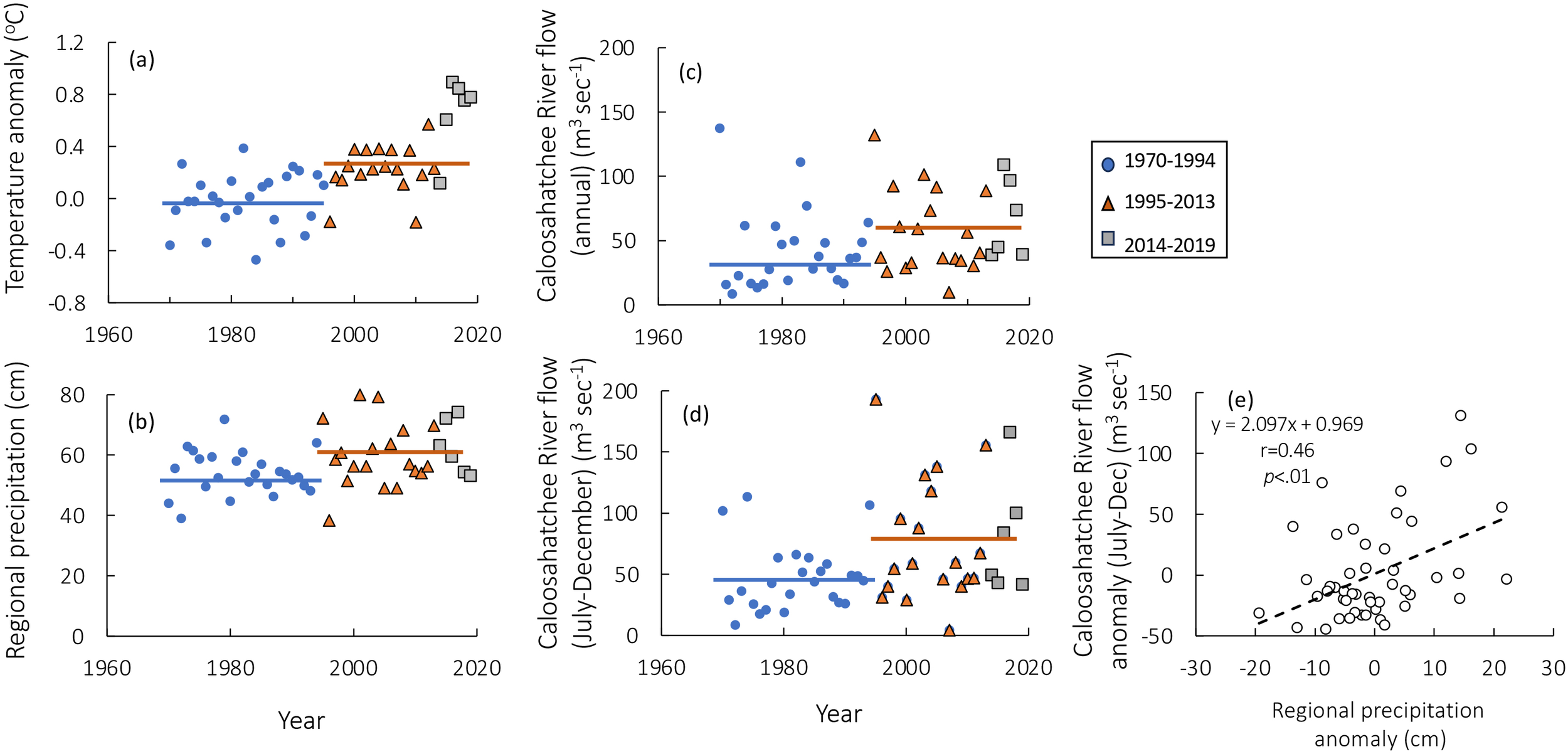
(a) Average annual temperature anomaly for the Gulf of Mexico for the periods 1970-1994 (blue circles), 1995-2013 (orange triangles) and 2014-2019 (gray squares). (b) Average annual regional precipitation for the same time periods. (c) Average annual flow from the Caloosahatchee River (c) and (d) flow for the months of July through December (d) for the same time periods. (e) Correlation between regional precipitation anomalies and Caloosahatchee River flow anomalies (July-December). The blue and orange horizontal bars in (a–d) represent the means of 1970–1994 and 1995-2019, respectively. In (a–d), the years 2014–2019 are represented by different symbols but are included in the post-1995 averages.
Consistent with the notion that when ONI is negative precipitation is higher, the average annual precipitation data for the regional counties increased significantly in the years 1995–2019 compared to 1970-1994 (Figure 3b; mean 1970-1994 = 54.14 cm, mean 1995-2019 = 60.58 cm; p = .012, df=48). Moreover, more extreme events, including hurricanes are expected, and indeed, the number of hurricanes or tropical storms that resulted in in substantial precipitation for southwestern Florida increased from the period of 1970–1994 to the period of 1995-2019 (Supplementary Figure 1). Furthermore, the intensity of precipitation associated with these hurricanes was also higher than that seen in the pre-1995 hurricanes, with Hurricanes Fay (Aug. 2008) and Irma (Sept 2017) delivering precipitation in excess of 25 cm in many regions.
The Caloosahatchee River, a managed river system, has the highest flows during July to December, with increased pulse discharge during the dry season to avoid riverine salt water intrusion at that time. Caloosahatchee River flow has also increased in the years post 1994 compared to the years 1970-1994. When flows are averaged annually, the difference between these time periods is significant (Figure 3c; mean 1970-1994 = 40.90 m3sec-1; mean 1995-2019 = 58.77 m3sec-1; p = .048, df= 47), but even more so when only the months of July through December are considered (Figure 3d, mean 1970-1994 = 47.2 m3 sec-1; mean 1995-2019 = 77.0 m3 sec-1; p = .010, df=47). Caloosahatchee River flow is a function of local precipitation and of Lake Okeechobee management actions, that is, planned releases from the lake to the river. Thus, regional precipitation anomalies are significantly related to Caloosahatchee River flow anomalies for the months of July-December (Figure 3e; r=0.46, df=47, p <.001).
3.2 Bloom severity changes
The number of months per decade with elevated BSI scores has increased over time (Figure 4). The number of months with an average BSI >2 (for blooms >100,000 cells L-1) increased from <15 in the 1970s and 1980s to >30 in the 2000s and 2010s, while months with a BSI >4 increased from <5 through the 1990s, to >10 after 2000 (Figure 4).
Figure 4
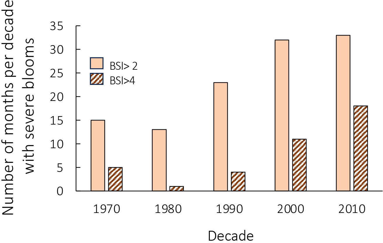
Number of months per decade with an average bloom severity index (BSI, cell density >100,000 cells L-1) >2 (light brown bars) and with a BSI >4 (brown striped bars), based on Stumpf et al. (2022).
During the first half of the time series (1970-1994), there was no relationship between annual average BSI (including all blooms with a positive severity score) and water temperature anomalies (Figure 5a). However, after 1995, BSI was positively and significantly (r=0.56, df =23 p = .003) related to the increase in temperature anomaly (Figure 5b). Similarly, the annual average bloom duration showed no relation with temperature in the 1970–1994 period but was positively and significantly related in the latter years (Figures 5c,d; r= 0.44, df=22, p = .003).
Figure 5
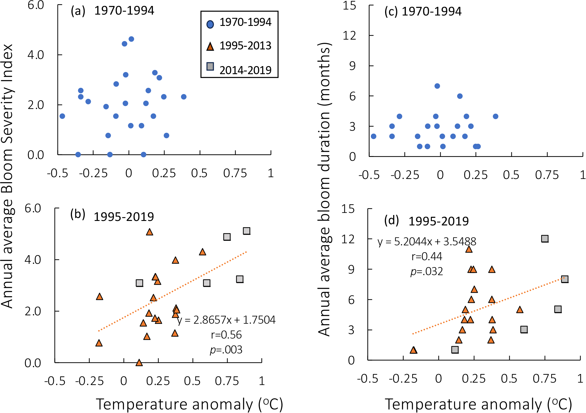
(a) Annual average Bloom Severity Index (BSI, cell density >100,000 cells L-1) as a function of temperature anomaly for 1970–1994 and (b) for the time period 1995-2019. (c, d) Average annual bloom duration (months) as a function of temperature anomaly for the same time periods. Note that there was no significant relationship for either bloom metric for the first half of the time series, but during the second half of the time series, the relationships were highly significant. In (b, d), orange triangles represent data from 1995–2013 and gray squares represent data from 2014–2019 but all data are included in the regressions.
The relationships between annual average BSI (including all blooms with a positive severity score) and bloom duration and late summer/fall Caloosahatchee River flows (in the months when blooms are most typical, July to December) are more complicated than the relationships with temperature (Figure 6). All relationships were significant for all time periods, but there were differences. In the early years, flows rarely exceeded 100 m3 sec-1 and there were no blooms with a BSI >2 and only two blooms had a duration greater than five months (Figures 6a, c). In the latter years, annual average BSI values were correlated with the Caloosahatchee River flow, which reached 200 m3 sec-1 (Figure 6b; r= 0.46, df=23, p = .003), but the relationship with bloom duration was even stronger (Figure 6d; r=0.63, df=22; p = .001). Indeed, the slope of the relationship post 1995 between bloom duration and July-December flows was 1.47 times that of the earlier time period. During this latter period, there were numerous blooms lasting more than eight months, all associated with river flows >100 m3 sec-1.
Figure 6
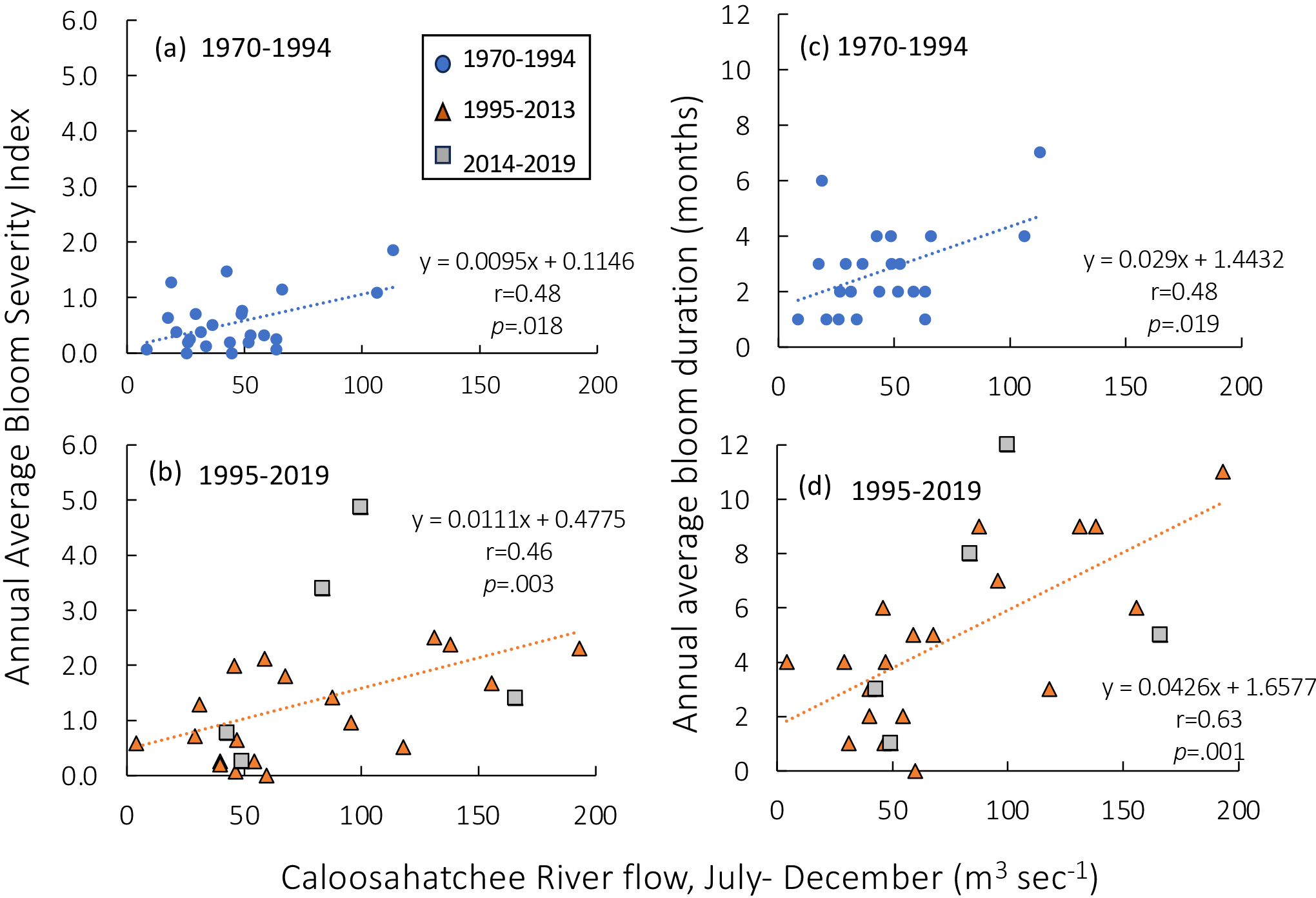
(a) Annual average Bloom Severity Index (BSI, cell density >100,000 cells L-1) as a function of the Caloosahatchee River flow (months of July-December only) for 1970–1994 and (b) for the time period 1995-2019. (c, d) Average annual bloom duration (months) as a function of the Caloosahatchee River flow (months of July-December only) for the same time periods. Note that all relationships were significant, but that between bloom duration and flow for the recent time period was the strongest. In (b, d), orange triangles represent data from 1995–2013 and gray squares represent data from 2014–2019 but all data are included in the regressions.
3.3 Fertilizer use, population growth and the regional human footprint
Long term consistent nutrient data are not available for the full time course examined here (1970-2019), and thus proxies are used as indicators of nutrient export. The watersheds of the Tampa Bay, and of the Peace and Caloosahatchee Rivers have changed from rural farms to heavily populated areas (Figure 7). From the 1970s through the mid 1990s, use of nitrogenous fertilizer increased, parallel to the global increase of fertilizer use. Urbanization of these regions began displacing farms and thus farm and nonfarm use of N-based fertilizers decreased from the mid-1990s (Figures 7b, f, j). Applying the N footprint multiplier (Leach et al., 2012) to the regional population census data, the increase in N is clear: it increased from roughly 40,000 tonnes/yr in the Tampa Bay region and from about 10,000 tonnes/yr in the other river watersheds in the 1970s to values roughly four-fold greater currently (Figures 7c, g, k).
Figure 7
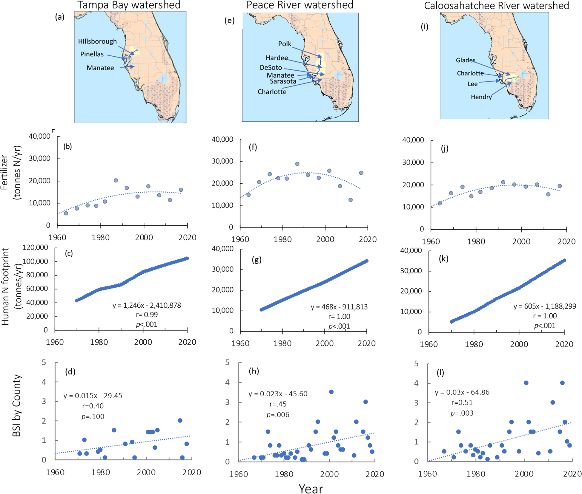
(a) The watershed of Tampa Bay; (b) Nitrogen fertilizer use for the Tampa Bay counties indicated over time; panel (c) human nitrogen footprint for these counties over time; and (d) annual BSI for Pinellas County. (e, f, g) As for (a–c) except for the Peace River watershed; (h) annual BSI for Manatee and Sarasota Counties. Panels (i–k) as for (a–c) except for the Caloosahatchee River watershed; (l) annual BSI for Lee and Charlotte Counties. Fertilizer data are reproduced from Falcone (2021); BSI data are based on blooms of >100,000 cells L-1 as reported by Li et al. (2025).
Annual BSI values for blooms >100,000 cells L-1 by county (based on Li et al., 2025) had somewhat different trends. The increases over time for Pinellas County (Figure 7d) were not significant, while those for Manatee and Sarasota Counties (Figure 7h) and for Lee and Charlotte Counties (Figure 7l) were highly significant (p = .006 and.003, respectively).
Annually, the anthropogenic N load (without the input of tourism) for each watershed for the total time period considered (1970-2019) correlates with the number of blooms with a BSI >2 per year (Figures 8a–c), but this relationship strengthens greatly (to r values of 0.92-0.94) when these relationships are based on 5-year averages rather than annual averages (Figures 8d–f).
Figure 8
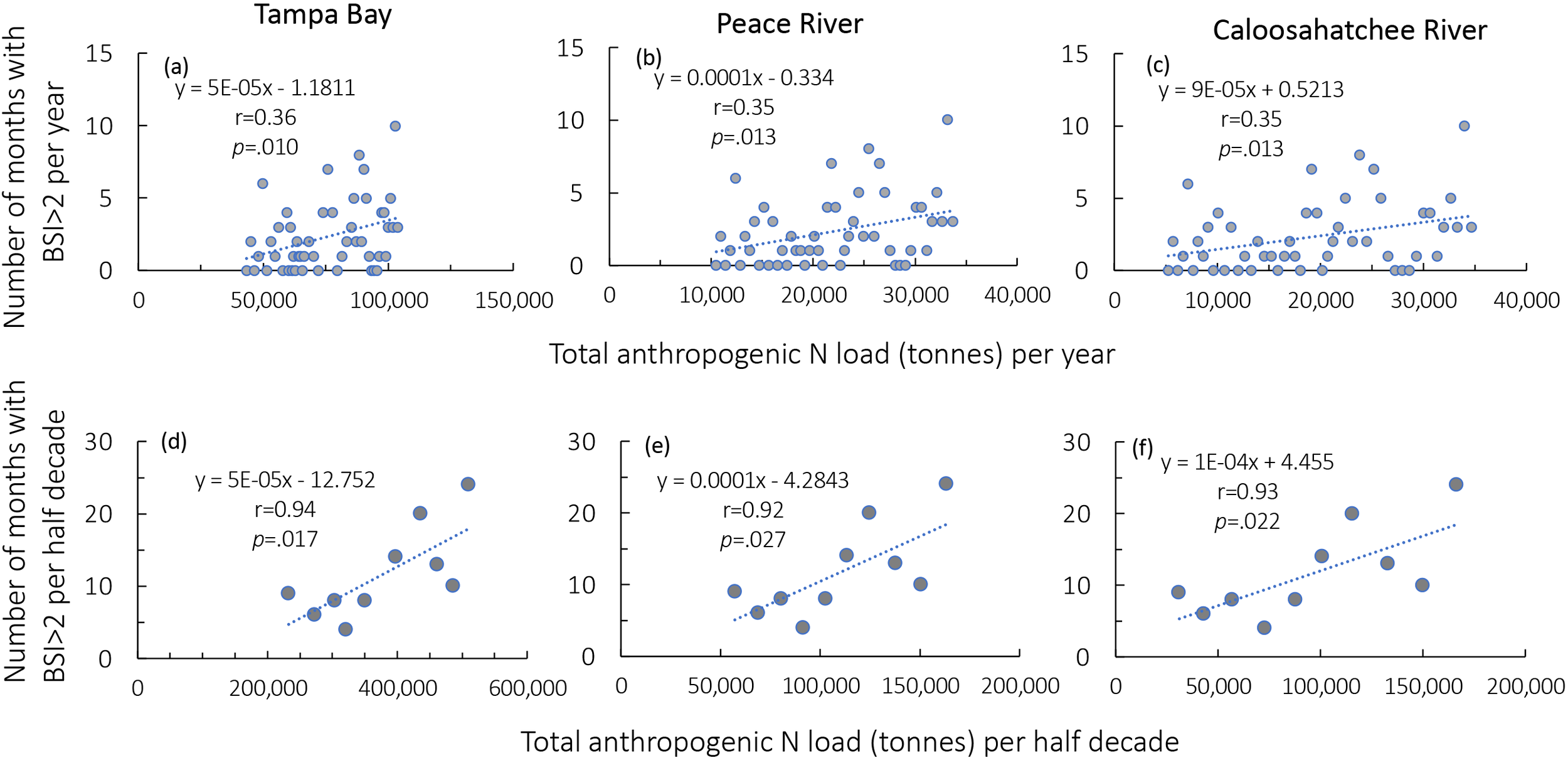
(a–c) Number of months per year with a Bloom Severity Index (BSI, cell density >100,000 cells L-1) >2 in relation to the estimate annual anthropogenic nitrogen footprint (calculated based on interpolated population for the Tampa Bay, Peace River and Caloosahatchee River watersheds), as based on Leach et al. (2012). (d–f) the same relationships as in (a–c), except the bloom months and the N loads are the cumulative values per half decade rather than per year. All relationships were significant at p <.05 (panels (a–c, df= 48; panels (d–f), df= 9). Note the increase in the coefficients of determination in the 5-year average relationships compared to the annual relationships.
4 Discussion
Blooms of Karenia brevis have increased over time in both duration and in severity associated with changes in climate (temperature and precipitation), river flow, and with the increased anthropogenic N footprint. The shift to more intense and longer blooms occurred coincident with the ONI shift in 1995 from a net positive ONI to one that was negative. A secondary shift appears to have occurred in 2014 again to a more positive ONI. These changes are consistent with reports of a transition to a negative phase of the Pacific Decadal Oscillation in the mid 1990s (e.g., Dong and Dai, 2015; Ellis and Marston, 2020; Zhang et al., 2023) and the more recent shift in North Atlantic in 2013 (e.g., Ren et al., 2023; Di Lorenzo et al., 2023; Kléparski et al., 2024). Stumpf et al. (2022) also described a break point in 1995, but without ascribing climatic changes, noted that wind patterns changed before and after this time. These analyses contrast with the conclusions drawn by Anderson et al. (2021) based only on toxin reports, that the 30-year trends in K. brevis and impacts over time were not significant.
Temperature changes were highly predictive of bloom severity and duration in the post-1995 era (Figure 5). Not only are waters warmer throughout the year, but periods of cooling, especially in the winter months, are also less (Glibert et al., 2025). These results are also consistent with the findings of Medina et al. (2020, 2022) and Tomasko et al. (2024), albeit for different time periods, showing that bloom intensity and duration is related to the Caloosahatchee River flow. Indeed, the flows for the second half of the year correlated strongly with bloom duration in the years post 1995 (Figure 6d).
The relationships herein between K. brevis bloom and estimated anthropogenic N loading based on the human footprint not only underscore the importance of land-based nutrients in supporting the maintenance stages of blooms but also shed light on why the earlier debates were inconclusive. These results demonstrate that conditions have changed significantly since the 1970s and 1980s–the period that many of the earlier studies (e.g., Walsh et al., 2006; Vargo et al., 2004, 2008, Anderson et al., 2008) relied upon. Higher precipitation enhances river flow (Figure 3e), that, together with more people and their associated nutrients, leads to increased nutrient runoff. The human N footprint has quadrupled since 1970, and the relationship between BSI duration and total anthropogenic load from 1970 to present is significant and direct (Figures 6, 7). The results reported here, although for a different time period, are consistent with Brand and Compton (2007) with respect to the general notion of the impact of anthropogenic N.
The human N footprint reported here should, in fact, be viewed as a conservative estimate, as these annual per-capita N values do not include the contribution of tourists (Supplementary Figure 2), which have been estimated to have increased from 20,000,000 annually in 1970 to ~100,000,000 million or more by 2019 (Harrington et al., 2017; Macdonald et al., 2023). Much of this tourism is focused around coastal and beach regions. In fact, it was estimated in 2012 that Florida had 810 million beach day visits (Macdonald et al., 2023).
It is of note that the trends for BSI for Pinellas County were not significant over time and, indeed, BSI values were lower than those reported for Manatee and Sarasota Counties and for Lee and Charlotte Counties (Figure 7). Two factors may have contributed to this trend. First, blooms are less common in the low salinity, estuarine waters of upper Tampa Bay. Also, aggressive N management strategies were implemented for Tampa Bay in the 1990s (Greening and Janicki, 2006) and may have helped to curb bloom frequency.
Long term nutrient concentration data for the West Florida Shelf are limited, and loads cannot be fully estimated from concentrations alone. Julian and Osborne (2018) reported total N (TN) loads for the Caloosahatchee River at Site 79 for much of the time periods covered here. Those data indeed do show a relationship, including a time-lagged relationship with bloom severity (Glibert et al., 2025). However, this record of TN does not capture the full anthropogenic input of N. Lu et al. (2020) demonstrated that extreme events and increased precipitation has occurred in the northern Gulf of Mexico, the Mississippi-Atchafalaya basin since 2000, delivering about 1/3rd of annual precipitation and thus 1/3 of total N. Rainwater measured in Sarasota has been shown to have dissolved inorganic N concentrations ranging from 5.8 –85 μmol L-1 (NH4+ concentrations ranging from 2.1 – 29.0 μmol L-1 and NO3- concentrations ranging from 3.7 –56.0 μmol L-1; Dillon and Chanton, 2005). The latter authors, using δ15N measurements of the dissolved N, found elevated values in stormwater and estimated that stormwater could deliver as much as 45% of the N load to Sarasota Bay. Muni-Morgan et al. (2024) recently reported large contributions of organic N to waters of Tampa Bay, especially during storm and extreme events. It is also of note that Charlotte County, which straddles the watersheds of the Caloosahatchee River and that of the Peace River, has a high concentration of septic systems, the effluent of which has been suggested to contribute surface and groundwater nutrients that contribute to maintenance and/or intensification of blooms (Brewton et al., 2022). Cooper et al. (2024) summarized land use land cover changes in the Lake Okeechobee watershed since the mid 1980s and highlighted the increased land application of treated effluent in the region. Collectively, these inputs would not be fully reflected routinely as NO3- or TN in the river or coastal water sites commonly monitored. Accordingly, Turner et al. (2006) and Anderson et al. (2008) both reported that while NO3- concentrations increased in the decades before 1960, concentrations have not increased since in the headwaters of the Caloosahatchee River and in the Caloosahatchee River mouth. These under-measured nutrient sources supplement the many nutrient sources that can support K. brevis blooms (Heil et al., 2014), including Trichodesmium N2 fixation, mixotrophic consumption of picoplankton, benthic flux, release of nutrients from dead fish killed by K. brevis, riverine nutrient loading and groundwater discharges (Vargo et al., 2008; Glibert et al., 2009; Heil et al., 2014; Dixon et al., 2014; O’Neil et al., 2024, Ahn and Glibert, 2024, Hu et al., 2005).
Blooms, which historically were considered a fall or winter phenomenon, are now increasingly expanding their duration (Figure 5; Glibert et al., 2025). This was the case for the blooms that persisted through the summer months in 2018–2019 and 2020-2021 (Figure 1). Blooms that can transition from the nutrient-limited spring through the summer may be able to thrive if provided an additional nutrient source in spring, when blooms might otherwise experience nutrient limitation and potentially temperature stress as the season progresses. In 2021, a major nutrient injection into Tampa Bay, Florida, occurred over two weeks in April following the breach of a wastewater holding pond from an abandoned P mining plant. Enhanced sediment release of NH4+ during the weeks following, and summer remineralization of dissolved organic N provided sufficient regenerated N to support slow-growing K. brevis through the otherwise stressful summer (Beck et al., 2022; Chen et al., 2023). Additional nutrients supporting early summer growth were supplied by Hurricane Elsa in June 2021 (Figure 1).
The Gulf of Mexico is warming at one of the fastest rates in the coastal US, at a rate of 0.19°C decade (Alexander et al., 2020, Maul and Sims, 2007), and this same trend is reflected in the inshore waters, as evidence by the comparison of the Gulf of Mexico trends with those of the regional Sarasota waters. The warm atmosphere and exceptionally warm waters make conditions more conducive for more intensive storms and hurricanes that deliver greater precipitation (Supplementary Figure 1). Higher precipitation and stronger hurricanes have occurred more frequently since 1998 relative to the prior decades (Knutson et al., 2019). While these higher precipitation events result in enhanced runoff events, bringing nutrients that propel the blooms, they do not appear to reduce salinities substantially to levels outside of the growth optimum for K. brevis. Once the river plumes spread over the shelf, the salinity increases quickly due to mixing (Chen and Li, 2025). This is unlike the condition of the more shallow Florida Bay where precipitation events and droughts can lead to highly variable and stressful salinity regimes (Kelble et al., 2007).
Recent analyses by Milbrandt et al. (2021) and Turley et al. (2022) have shown that large K. brevis blooms are associated with increased hypoxia. Recent hypoxic events occurred concurrently with extreme K. brevis blooms that have lasted throughout the summer. During the K. brevis bloom of 2005, hypoxia was recorded (Hu et al., 2005; Dupont et al., 2010), along with considerable amounts of dead gag grouper. It has been suggested that hypoxia occurring in parallel to a red tide is more likely to occur with warmer ocean temperatures, with its lower O2 solubility, and increased fluxes of nutrients and fresh water to the Gulf of Mexico after hurricanes (Milbrandt et al., 2021). Recasting the Turley et al. (2022) data in comparison with the BSI values for the same time periods, it can be seen that the highest BSI values are indeed associated with greater hypoxia (Figure 9). It is also likely that hypoxia is substantially underestimated on the West Florida Shelf due to the fact that oceanographic casts near the seafloor are comparatively rare and not necessarily regionally detailed.
Figure 9

Relationship between minimum bottom water oxygen for the eastern Gulf of Mexico (from Turley et al., 2022) and Bloom Severity Index (from Stumpf et al., 2022, based on cell concentrations >100,000 cells L-1) for all dates for which both data are available. This analysis covers only 2003-2019. Orange squares represent years from 2003-2014. Gray squares represent data from 2014-2019. When BSI values were <6, there was no significant relationship with bottom water dissolved oxygen. Moreover, there was no relationship when the years 2003–2014 only are considered. However, after 2014, a significant negative relationship with bottom water dissolved oxygen was apparent, underscoring the role that recent severe blooms play in deoxygenation.
5 Conclusions
The impact of changes in temperatures and increases in human population, with its associated N pollution, and river flow can no longer be ignored as factors contributing to the increased frequency and severity of K. brevis blooms. The combination of hypoxia, toxic K. brevis blooms, and warming will multiply the stress and pressure on higher trophic level species inhabiting on the West Florida Shelf, the home to one of the nation’s most diverse and productive ecosystems supporting fisheries and aquaculture important to the economy of southwest Florida (Dupont et al., 2010; Bohnsack, 2011; DiLeone and Ainsworth, 2019; Glibert et al., 2022). The challenges for management to control K. brevis blooms in the face of climate stresses and anthropogenic pressures have increased and will only increase further in the future. To reduce bloom severity and duration, stressors that can be controlled, including N loads and releases from the Caloosahatchee River, are needed more than ever to counteract the increasing pressures from climate, a stressor much more difficult to control.
Statements
Data availability statement
The original contributions presented in the study are included in the article/Supplementary Material. Further inquiries can be directed to the corresponding author.
Author contributions
PG: Visualization, Formal Analysis, Writing – original draft, Funding acquisition, Conceptualization, Methodology, Investigation, Writing – review & editing. CH: Project administration, Data curation, Methodology, Formal Analysis, Writing – review & editing, Investigation, Conceptualization, Funding acquisition. ML: Formal Analysis, Funding acquisition, Writing – review & editing, Investigation, Conceptualization.
Funding
The author(s) declared that financial support was received for this work and/or its publication. Funding for this work was provided by NOAA awards NA19NOS4780183 and NA23NOS4780286 and NSF Award 2309082 to PMG, CAH and ML.
Acknowledgments
This is contribution number 6488 from the University of Maryland Center for Environmental Science and 1142 from the NOAA ECOHAB Program.
Conflict of interest
The author(s) declared that this work was conducted in the absence of any commercial or financial relationships that could be construed as a potential conflict of interest.
The author ML declared that they were an editorial board member of Frontiers, at the time of submission. This had no impact on the peer review process and the final decision.
Generative AI statement
The author(s) declare that no Generative AI was used in the creation of this manuscript.
Any alternative text (alt text) provided alongside figures in this article has been generated by Frontiers with the support of artificial intelligence and reasonable efforts have been made to ensure accuracy, including review by the authors wherever possible. If you identify any issues, please contact us.
Publisher’s note
All claims expressed in this article are solely those of the authors and do not necessarily represent those of their affiliated organizations, or those of the publisher, the editors and the reviewers. Any product that may be evaluated in this article, or claim that may be made by its manufacturer, is not guaranteed or endorsed by the publisher.
Supplementary material
The Supplementary Material for this article can be found online at: https://www.frontiersin.org/articles/10.3389/fmars.2026.1769349/full#supplementary-material
References
1
Ahn S. Glibert P. M. (2024). Temperature-dependent mixotrophy in natural populations of the toxic dinoflagellate Karenia brevis. Water16, 1555. doi: 10.3390/w16111555
2
Alexander M. A. Shin S. K. Scott J. D. Curchitser E. Stock C. (2020). The response of the Northwest Atlantic Ocean to climate change. J. Clim.33, 405–428. doi: 10.1175/JCLI-D-19-0117.1
3
Anderson D. M. Burkholder J. M. Cochlan W. P. Glibert P. M. Gobler C. J. Heil C. A. et al . (2008). Harmful algal blooms and eutrophication: Examining linkages from selected coastal regions of the United States. Harmful Algae8, 39–53. doi: 10.1016/j.hal.2008.08.017
4
Anderson D. M. Fensin E. Gobler C. J. Hoegland A. E. Hubbard K. A. Kulis D. M. et al . (2021). Marine harmful algal blooms (HABs) in the United States: history, current status and future trends. Harmful Algae102, 101975. doi: 10.1016/j.hal.2021.101975
5
Beck M. W. Altieri A. Angelini C. Burke M. C. Chen J. Chin D. W. et al . (2022). Initial estuarine response to inorganic nutrient inputs from a legacy mining facility adjacent to Tampa Bay, Florida. Mar. Poll Bull.178, 11398. doi: 10.1016/j.marpolbul.2022.113598
6
Bell G. D. Chelliah M. (2006). Leading tropical modes associated with interannual and multidecadal fluctuations in north atlantic hurricane activity. J. Climate19, 590–612. doi: 10.1175/JCLI3659.1
7
Bohnsack J. A. (2011). Impacts of Florida coastal protected areas on recreational world records for spotted seatrout, red drum, black drum, and common snook. Bull. Mar. Sci.87, 939–970. doi: 10.5343/bms.2010.1072
8
Brand L. E. Compton A. (2007). Long-term increase in Karenia brevis abundance along the Southwest Florida Coast. Harmful Algae6, 232–252. doi: 10.1016/j.hal.2006.08.005
9
Brewton R. A. Kreiger L. B. Tyre K. N. Baladi D. Wilking L. E. Herren L. W. et al . (2022). Septic system–groundwater–surface water couplings in waterfront communities contribute to harmful algal blooms in Southwest Florida. Sci. Tot Environ.837, 155319. doi: 10.1016/j.scitotenv.2022.155319
10
Briceño H. O. Boyer J. N. (2010). Climactic controls on nutrients and phytoplankton biomass in asub-tropical estuary, Florida Bay, USA. Estuaries Coasts33, 541–553. doi: 10.1007/s12237-009-9189-1
11
Brown A. F. M. Dortch Q. Van Dolah F. M. Leighfield T. A. Morrison W. Thessen A. E. et al . (2006). Effect of salinity on the distribution, growth, and toxicity of Karenia spp. Harmful Algae5, 199–212. doi: 10.1016/j.hal.2005.07.004
12
Chen Y. Li M. (2025). Impact of hurricane ian, (2022) on Karenia brevis bloom on the West Florida Shelf. Geophysical Res. Lett.52, e2024GL113500. doi: 10.1029/2024GL113500
13
Chen Y. Li M. Glibert P. M. Heil C. A. (2023). MurKy waters: Modeling the succession from r to K strategists (diatoms to dinoflagellates) following a nutrient spill from a mining facility in Florida. Limnol. Oceanog.68, 2288–2304. doi: 10.1002/lno.12420
14
Cooper R. Z. Ergas S. J. Nachabe M. (2024). Multi-decadal nutrient management and trends in two catchments of Lake Okeechobee. Resources13, 28. doi: 10.3390/resources13020028
15
DiLeone A. M. G. Ainsworth C. H. (2019). Effects of Karenia brevis harmful algal blooms on fish community structure on the West Florida Shelf. Ecol. Modell.392, 250–267. doi: 10.1016/j.ecolmodel.2018.11.022
16
Dillon K. S. Chanton J. P. (2005). Nutrient transformations between rainfall and stormwater runoff in an urbanized coastal environment: Sarasota Bay, Florida. Limnol. Oceanogr.50, 62–69. doi: 10.4319/lo.2005.50.1.0062
17
Di Lorenzo E. Xu T. Zhao Y. Newman M. Capotondi A. Stevenson S. et al . (2023). Modes and mechanisms of Pacific decadal-scale variability. Ann. Rev. Mar. Sci.15, 249–275. doi: 10.1146/annurev-marine-040422-084555
18
Dixon L. K. Murphy P. J. Becker N. M. Charniga C. M. (2014). The potential role of benthic nutrient flux in support of Karenia blooms in west Florida (USA) estuaries and the nearshore Gulf of Mexico. Harmful Algae38, 30–39. doi: 10.1016/j.hal.2014.04.005
19
Dixon L. K. Steidinger A. (2002). “ Correlation of Karenia brevis in the eastern Gulf of Mexico with rainfall and riverine flow,” in Harmful Algae 2002, Proceedings of the Xth International Conference on Harmful Algae. Eds. SteidingerK. A.LandsbergJ. H.TomasC. R.VargoG. A. ( Florida Fish and Wildlife Conservation Commission, Florida Institute of Oceanography, and Intergovernmental Oceanographic Commission of UNESCO, St. Petersburg, FL), 29–31.
20
Dong B. Dai A. (2015). The influence of the interdecadal Pacific Ocean oscillation on temperature and precipitation over the globe. Clim. Dyn.45, 2667–2681. doi: 10.1007/s00382-015-2500-x
21
Dupont J. M. Hallock P. Jaap W. C. (2010). Ecological impacts of the 2005 red tide on artificial reef epibenthic macroinvertebrate and fish communities in the eastern Gulf of Mexico. Mar. Ecol. Progr. Ser.415, 189–200. doi: 10.3354/meps08739
22
Ellis A. W. Marston M. L. (2020). “ Late 1990s cool season climate shift in eastern North America,” in Climate Change162, 1385–1398. doi: 10.1007/s10584-020-0227988-z
23
Falcone J. A. (2021). Tabular county-level nitrogen and phosphorus estimates from fertilizer and manure for approximately 5-year periods from 1950 to 2017: U.S. Geological Survey Data release. doi: 10.5066/P9VSQN3C
24
Galloway J. N. Winiwarter W. Leip A. Leach A. M. Bleeker A. Erisman J. W. (2014). Nitrogen footprints: past, present and future. Environ. Res. Lett.9, 115003. doi: 10.1088/1748-9326/9/11/115003
25
Glibert P. M. Burkholder J. M. Kana T. M. Alexander J. A. Schiller C. Skelton H. (2009). Grazing by Karenia brevis on Synechococcus enhances their growth rate and may help to sustain blooms. Aq. Microb. Ecol.55, 17–30. doi: 10.3354/ame01279
26
Glibert P. M. Cai W.-J. Hall E. Li M. Main K. Rose K. et al . (2022). Stressing over the complexities of multiple stressors in marine and estuarine systems. Ocean-Land-Atmos. Res.2022, 9787258. doi: 10.34133/2022/9787258
27
Glibert P. M. Heil C. A. Li M. (2025). More sustained, more severe blooms and shifting monthly patterns of the toxigenic dinoflagellate Karenia brevis on the West Florida Shelf. Harmful Algae150, 102967. doi: 10.1016/j.hal.2025.102967
28
Gray W. M. (1984). Atlantic seasonal hurricane frequency, Part I: El Niño and 30 mb quasi-biennial oscillation influences. Mon. Wea. Rev.115, 1649–1668. doi: 10.1175/1520-0493(1984)112<1649:ASHFPI>2.0.CO;2
29
Greening H. Janicki A. (2006). Toward reversal of eutrophic conditions in a subtropical estuary: water quality and seagrass response to nitrogen loading reductions in tampa bay, florida, USA. Envir. Mngmt.38, 163–178. doi: 10.1007/s00267-005-0079-4
30
Harrington J. Chi H. Gray L. P. (2017). “ Florida tourism,” in Florida’s Climate: Changes, Variations, & Impacts. (Gainesville, FL: Florida Climate Institute). Available online at: http://purl.flvc.org/fsu/fd/FSU_libsubv1_scholarship_submission_1515510103_158bad4e (Accessed September 12, 2025).
31
Haverkamp D. Steidinger K. A. Heil C. A. (2004). “ HAB monitoring and databases: the Karenia brevis example,” in Harmful Algae Management and Mitigation. Eds. HallS.EtherrdgeS.AndersonD.KleindinstJ.ZhuM.ZouY. ( APEC Publication 204-MR-04.2, Asia-Pacific Economic Cooperation, Singapore).
32
Heil D. C. (2009). Karenia brevis monitoring, management, and mitigation for Florida molluscan shellfish harvesting areas. Harmful Algae8, 608–610. doi: 10.1016/j.hal.2008.11.007
33
Heil C. A. Amin S. A. Glibert P. M. Hubbard K. A. Li M. Martínez Martínez J. et al . (2022). “ Termination patterns of Karenia brevis blooms in the eastern Gulf of Mexico,” in Proceedings of the International Harmful Algal Bloom Conference, La Paz, Mexico, October 2021. doi: 10.5281/zenodo/7034923
34
Heil C. A. Dixon L. K. Hall E. Garrett M. Lenes J. M. O'Neil J. M. et al . (2014). Blooms of Karenia brevis (Davis) G. Hansen & Ø. Moestrup on the West Florida Shelf: Nutrient sources and potential management strategies based on a multi-year regional study. Harmful Algae38, 127–140. doi: 10.1016/j.hal.2014.07.016
35
Heil C. A. Steidinger K. A. (2009). Monitoring, management, and mitigation of Karenia blooms in the eastern Gulf of Mexico. Harmful Algae8, 611–617. doi: 10.1016/j.hal.2008.11.006
36
Hu C. Muller-Karger F. E. Swarzenski P. W. (2005). Hurricanes, submarine groundwater discharge, and Florida’s red tides. Geophys. Res. Letts.33, 5. doi: 10.1029/2005GL025449
37
Hurrel J. W. (1995). Decadal trends in the North Atlantic Oscillation: Regional temperatures and precipitation. Science269, 676–679. doi: 10.1126/science.269.5224.676
38
Julian P. Osborne T. Z. (2018). From lake to estuary, the tale of two waters: a study of aquatic continuum biogeochemistry. Envir. Monitor. Assess.190, 96. doi: 10.1007/s10661-017-6455-8
39
Kelble C. R. Johns E. M. Nuttle W. K. Lee T. N. Smith R. H. Ortner P. B. (2007). Salinity patterns of Florida Bay. Est. Coast. Shelf Sci.71, 318–334. doi: 10.1016/j.ecss.2006.08.006
40
Kleparski L. Beaugrand G. Ostle C. Edwards M. Skogen M. D. Djeghri N. et al . (2024). Ocean climate and hydrodynamics drive decadal shifts in Northeast Atlantic dinoflagellates. Glob. Change Biol.30, e17163. doi: 10.1111/gcb.17163
41
Knutson T. R. Camargo S. J. Chan J. Emanuel K. Ho C.-H. Kossin J. et al . (2019). Tropical cyclones and climate change assessment: Part I. Detection and attribution. Bull. Amer. Meteor. Soc100, 1987–2007. doi: 10.1175/BAMS-D-18-0189.1
42
Leach A. M. Galloway J. N. Bleeker A. Erisman J. W. Kohn R. Kitzes J. (2012). A nitrogen footprint model to help consumers understand their role in nitrogen losses to the environment. Environ. Dev.1, 40–66. doi: 10.1016/j.envdev.2011.12.005
43
Li M. F. Glibert P. M. Lyubchich V. (2021). Machine learning classification algorithms for Predicting Karenia brevis blooms on the West Florida Shelf. J. Mar. Sci. Eng.9, 999. doi: 10.3390/jmse9090999
44
Li Y. Litaker W. Stumpf R. Kirkpatrick B. Hubbard K. Harrison K. (2025). “ An updated high-resolution, site-specific Karenia brevis bloom severity index and associated respiratory irritation impacting the southwest Florida coast,” in UNESCO Harmful Algae News NO.80 ( Zenodo), 5–9. doi: 10.5281/zenodo.17220214
45
Liu Y. Weisberg R. H. (2012). Seasonal variability on the west florida shelf. Prog. Oceanogr104, 80–98. doi: 10.1016/j.pocean.2012.06.001
46
Liu Y. Weisberg R. H. Lenes J. M. Zheng L. Hubbard K. Walsh J. J. (2016). Offshore forcing on the ‘pressure point” of the West Florida Shelf: anomalous upwelling and its influence on harmful algal blooms. J. Geophys Res. Oceans. 121, 5501–5515. doi: 10.1002/2016JC011938
47
Lu C. Zhang J. Tian H. Crumpton W. G. (2020). Increased extreme precipitation challenges nitrogen load management to the Gulf of Mexico. Nat. Comm Earth Environ.1, 21. doi: 10.1038/s43247-020-00020-7
48
Macdonald C. Turffs D. McEntee K. Elliot J. Wester J. (2023). The relationship between tourism and the environment in Florida, USA: A media content analysis. Ann. Tourism Res. Empir. Insights4, 100092. doi: 10.1016/j.annale.2023.100092
49
MacNally R. Hart B. T. (1997). Use of CUSUM methods for water quality monitoring in storages. Environ. Sci. Technol.31, 2114–2119.
50
Magaña H. A. Villareal T. A. (2006). The effect of environmental factors on the growth rate of Karenia brevis (Davis) G. Hansen and Moestrop. Harmful Algae5, 192–198. doi: 10.1016/j.hal.2005.07.003
51
Manly B. F. J. Mackenzie D. I. (2003). CUSUM environmental monitoring in time and space. Environ. Ecol. Stats10, 231–247. doi: 10.1023/A:1023682426285
52
Maul G. A. Sims H. J. (2007). Florida coastal temperature trends: Comparing independent datasets. Florida Scientist70, 71–82.
53
Medina M. Huffaker R. Jawitz J. W. Muñoz-Carpena R. (2020). Seasonal dynamics of terrestrially sourced nitrogen influence Karenia brevis blooms of Florida’s southern Gulf Coast. Harmful Algae98, 101900. doi: 10.1016/j.hal.2020.101900
54
Medina M. Kaplan D. Milbrandt E. Tomasko D. Huffaker R. Angelini C. (2022). Nitrogen-enriched discharges from a highly managed watershed intensity red tide (Karenia brevis) blooms in southwest Florida. Sci. Tot. Environ.827, 154149. doi: 10.1016/j.scitotenv.2022.154149
55
Mesnil B. Petitgas P. (2009). Detection of changes in time series using CUSUM control charts. Aquat. Living Res.22, 187–192. doi: 10.1051/alr/2008058
56
Milbrandt E. C. Martignette A. J. Thompson M. A. Bartleson R. D. Phlips E. J. Badylak S. et al . (2021). Geospatial distribution of hypoxia associated with a Karenia brevis bloom. Est. Coast. Shelf Sci.259, 107446. doi: 10.1016/j.ecss.2021.107446
57
Muni-Morgan A. L. Lusk M. G. Heil C. A. (2024). Karenia brevis and Pyrodinium bahamense utilization of dissolved organic matter in urban stormwater runoff and rainfall entering Tampa Bay, Florida. Water16, 1448. doi: 10.3390/w16101448NOAA2015
58
O’Neil J. M. Heil C. A. Glibert P. M. Solomon C. M. Greenwood J. Greenwood J. G. (2024). Plankton community changes and nutrient dynamics associated with blooms of the pelagic cyanobacterium Trichodesmium in the Gulf of Mexico and the Great Barrier Reef. Water16, 1663. doi: 10.3390/w16121663
59
Page E. S. (1954). Continuous inspection schemes. Biometrika41, 100–115. doi: 10.1093/biomet/41.1-2.100
60
Ren X. Liu W. Capotondi A. Amaya D. J. Holbrook N. J. (2023). The Pacific Decadal Oscillation modulated marine heatwaves in the Northeast Pacific during past decades. Commun. Earth Envir.4, 218. doi: 10.1038/s43247-023-00863-w
61
Sobrinho B. Glibert P. M. Lyubchich V. Heil C. A. Li M. (2022). “ Time series analysis of the Karenia brevis blooms on the West Florida Shelf: relationships with El Nino – Southern Oscillation (ENSO) and its rate of change,” in Proceedings of the International Harmful Algal Bloom Conference, La Paz, Mexico, October 2021. doi: 10.5281/zenodo/7036227
62
Steidinger K. A. (1975). Implications of dinoflagellate life cycles on initiation of Gymnodinium breve red tides. Envir Letts9, 129–139. doi: 10.1080/00139307509435842
63
Steidinger K. A. (2009). Historical perspective on Karenia brevis red tide research in the Gulf of Mexico. Harmful Algae8, 549–561. doi: 10.1016/j.hal.2008.11.009
64
Stumpf R. P. Li Y. Kirkpatrick B. Litaker R. W. Hubbard K. A. Currier R. D. et al . (2022). Quantifying Karenia brevis bloom severity and respiratory irritation impact along the shoreline of Southwest Florida. PloS One17, e0260755. doi: 10.1371/journal.pone.0260755
65
Tester P. Steidinger K. A. (1997). Gymnodinium breve red tide blooms: Initiation, transport, and consequences of surface circulation. Limnol Oceanogr42, 1039–1051. doi: 10.4319/lo.1997.42.5_part_2.1039
66
Tomasko D. Landau L. Suau S. Medina M. Hecker J. (2024). An evaluation of the relationships between the duration of red tide (Karenia brevis) blooms and watershed nitrogen loads in southwest Florida (USA). Florida Scientist87, 61–72.
67
Turley B. D. Karnauskas M. Campbell M. D. Hanisko D. S. Kelble C. R. (2022). Relationships between blooms of Karenia brevis and hypoxia across the West Florida Shelf. Harmful Algae114, 102223. doi: 10.1016/j.hal.2022.102223
68
Turner R. E. Rabalais N. N. Fry B. Atilla N. Milan C. S. Lee J. M. et al . (2006). Paleo-indicators and water quality change in the Charlotte Harbor estuary (Florida). Limnol Oceanogr51, 518–533.doi: 10.4319/lo.2006.51.1_part_2.0518
69
Vargo G. A. (2009). A brief summary of the physiology and ecology of Karenia brevis Davis (G. Hansen and Moestrup comb. nov.) red tides on the West Florida Shelf and of hypotheses posed for their initiation, growth, maintenance, and termination. Harmful Algae8, 573–584. doi: 10.1016/j.hal.2008.11.002
70
Vargo G. A. Heil C. A. Ault D. N. Neely M. B. Murasko S. Havens J. et al . (2004). “ Four Karenia brevis blooms: A comparative analysis,” in Harmful Algae 2002, Proceedings of the Xth International Conference on Harmful Algae. Eds. SteidingerK. A.LandsbergJ. H.TomasC. R.VargoG. A. ( Florida Fish and Wildlife Conservation Commission, Florida Institute of Oceanography and Intergovernmental Oceanographic Commission of UNESCO, Paris), 14–16.
71
Vargo G. A. Heil C. A. Fanning K. A. Dixon K. A. Neely M. B. Lester K. et al . (2008). Nutrient availability in support of Karenia brevis blooms on the central West Florida Shelf: What keeps Karenia blooming? Cont. Shelf Res.28, 73–98. doi: 10.1016/j.csr.2007.04.008
72
Walsh J. J. Jolliff J. K. Darrow B. P. Lenes J. M. Milroy S. P. Remsen A. et al . (2006). Red tides in the Gulf of Mexico: where, when, and why? J. Geophys. Res.111, C11003. doi: 10.1029/2004JC002813
73
Walsh J. J. Weisberg R. H. Dieterle D. A. He R. Darrow B. P. Jolliff J. K. et al . (2003). Phytoplankton response to instrusions of slope water on the West Floirda Shelf: Models and observations. J. Geophys. Res. Oceans108 (c6). doi: 10.1029/2002JC001406
74
Walsh J. J. Steidinger K. A. (2001). Saharan dust and Florida red tides: the cyanophyte connection. J. Geophys Res. Oceans106, 11597–11612. doi: 10.1029/1999JC000123
75
Zhang S. Liu Y. Dong B. Sheng C. (2023). Decadal modulation of the relationship between tropical southern Atlantic SST and subsequent ENSO by Pacific decadal oscillation. Geophys. Res. Lett.50, e2023GL104878. doi: 10.1029/2023GL104878
Summary
Keywords
anthropogenic footprint, Bloom Severity Index, Florida red tide, Gulf of Mexico, Karenia brevis , time series
Citation
Glibert PM, Heil CA and Li M (2026) Climate shifts and anthropogenic footprints driving increased severity and duration of toxic Karenia brevis blooms in the Gulf of Mexico over the past ~50 years. Front. Mar. Sci. 13:1769349. doi: 10.3389/fmars.2026.1769349
Received
16 December 2025
Revised
24 January 2026
Accepted
26 January 2026
Published
16 February 2026
Volume
13 - 2026
Edited by
Sreenivasulu Ganugapenta, University of Malaysia Terengganu, Malaysia
Reviewed by
Fatin Izzati Minhat, University of Malaysia Terengganu, Malaysia
Željko Jaćimović, University of Montenegro, Montenegro
Updates
Copyright
© 2026 Glibert, Heil and Li.
This is an open-access article distributed under the terms of the Creative Commons Attribution License (CC BY). The use, distribution or reproduction in other forums is permitted, provided the original author(s) and the copyright owner(s) are credited and that the original publication in this journal is cited, in accordance with accepted academic practice. No use, distribution or reproduction is permitted which does not comply with these terms.
*Correspondence: Patricia M. Glibert, glibert@umces.edu
ORCID: Patricia M. Glibert, orcid.org/0000-0001-5690-1674; Cynthia A. Heil, orcid.org/0000-0001-9746-4132; Ming Li, orcid.org/0000-0003-1492-4127
Disclaimer
All claims expressed in this article are solely those of the authors and do not necessarily represent those of their affiliated organizations, or those of the publisher, the editors and the reviewers. Any product that may be evaluated in this article or claim that may be made by its manufacturer is not guaranteed or endorsed by the publisher.