Optimising complexity and learning for photonic reservoir computing with gain-controlled multimode fibres

Nonlinear photonics is a promising platform for neuromorphic hardware, offering high-speed processing, broad bandwidth, and scalable integration. Within this framework, Reservoir Computing (RC) and Extreme Learning Machines (ELM) are powerful approaches that leverage the dynamics of a complex nonlinear system to process information. In photonics, a key open challenge is controlling the nonlinear response required by photonic RC systems to tailor the photonic substrate (i.e., the physical implementation of the reservoir) to the specific task requirements. In this theoretical work, we propose a nonlinear photonic reservoir based on Erbium-Doped Multi-Mode Fibres (ED-MMF). In our approach, RC is implemented by structuring the pump and probe beams using phase-only spatial light modulators. Thanks to the nonlinear interactions between signal and pump modes within the gain medium, we show how the ED-MMF implements a tunable nonlinear transformation of the input field, where the degree of nonlinear coupling between different fibre modes can be controlled through easily accessible global parameters, such as pump and signal power. The ability to dynamically tune the degree of nonlinearity in our system enables us to identify the best operating conditions for our reservoir system across regression, classification, and time-series prediction tasks. We discuss the physical origin of the optimal regions by analysing the information theory and linear algebra properties of the readout matrix, unveiling a deep connection between the computational performance of the system and the Kolmogorov algorithmic complexity of the nonlinear features generated by the reservoir. Our results pave the way to developing optimised nonlinear photonic reservoirs leveraging structured complexity and controllable nonlinearity as fundamental design principles.

1 Introduction

Artificial Intelligence (AI) and Machine Learning (ML) techniques are transforming our ability to tackle complex scientific, engineering, and societal problems (Jumper et al., 2021). As model sizes continue to grow, the computational cost of training and inference has clearly surpassed the capacities of general-purpose digital processors (Amodei et al., 2018; Bhardwaj et al., 2025). To sustain progress, researchers are moving toward hardware acceleration, shifting key computational primitives, such as matrix-vector multiplication or artificial neuron (perceptron) layers, from software implementations in silico to physical processing in materio (Kudithipudi et al., 2025; Marković et al., 2020; Roy et al., 2019; Xu et al., 2024; Olivieri et al., 2025). A key open challenge in this area is the limited availability of fast and scalable reconfigurable hardware to enable on-device training, and most neuromorphic systems are deployed only at the inference stage (Marković et al., 2020; Merolla et al., 2014). As a compelling approach, physical Reservoir Computing (RC) exploits the complex dynamics of a physical system, such as an optical or electronic device or even a quantum system, to process data (Tanaka et al., 2019; Marković et al., 2020; McCaul et al., 2023; Nerenberg et al., 2025). In close analogy with echo state networks and liquid state machines (Jaeger and Haas, 2004; Maass, 2011), the physical system (reservoir) processes input signals through its dynamic response, and the target output is obtained by linear combination (i.e., linear regression) of specific measurements of the reservoir state (readout). This approach exploits the rich dynamics of the complex system to solve various tasks, ranging from signal processing to regression, classification, and prediction, without training or modifying the internal structure of the reservoir (Ghosh et al., 2019). As such, RC and its feed-forward variant, the Extreme Learning Machine (ELM), are appealing because only the final linear readout is trained, a strategy that greatly simplifies hardware implementation and eliminates the need to propagate errors through physical components (Tanaka et al., 2019; Wang D. et al., 2024).

In this context, nonlinear optical waves have emerged as a compelling substrate (i.e., the physical system embodying the reservoir) for physical reservoir computing (Brunner et al., 2025; McMahon, 2023; Pierangeli et al., 2021). Unlike standard neuromorphic photonic systems, where artificial neurons are mapped one-to-one to interconnected photonic devices, wave-based photonic reservoirs can encode and process information entirely in the optical domain, granting access to significant parallelism within single optical components (Shastri et al., 2021; Marcucci et al., 2020; Valensise et al., 2022; Wang Z. et al., 2024; Wang et al., 2024c). The computational capabilities of wave-based reservoirs rely on the interplay between complex wave interactions (e.g., in linear scattering media) and optical nonlinearity (e.g., cubic nonlinearities in optical fibres or nonlinear crystals) (Marcucci et al., 2020; Teğin et al., 2021; Valensise et al., 2022; Gigan, 2022; Hurtado et al., 2022; Shishavan et al., 2025). Intuitively, wave mixing and nonlinear interactions can be understood as the two ingredients required to implement a controlled nonlinear transformation of the input data, in close analogy with the combination of linear connections and activation functions in multilayer perceptrons (Dong et al., 2020a; Dong et al., 2020b; Pierangeli et al., 2020). Recent results suggest that wave-based reservoirs must exceed a specific degree of nonlinearity or configurational disorder to achieve effective learning (Marcucci et al., 2020; Pierro et al., 2023; Hary et al., 2025). The role of the reservoir is, in fact, to project the input data into a high-dimensional space of nonlinear features expressed by the observable degrees of freedom of the state of the system (Dale et al., 2019; McCaul et al., 2025a). However, in optics, nonlinearity and disorder are generally fixed by the geometric and material properties of the photonic device. Achieving a controllable degree of tunability could enable a single photonic device to adapt to different tasks, avoiding suboptimal performance that occurs when a reservoir is too linear or, conversely, chaotic (Wang et al., 2024d; Xia et al., 2024). In this context, a detailed analysis of the critical thresholds in nonlinearity and complexity required to perform computations is still critically missing, even though recent results in spin wave reservoirs suggest that nonlinearity, memory, and complexity need to be adapted to the specific task at hand (Gartside et al., 2022; Lee et al., 2024).

Within this framework, light-matter interactions in gain media provide an attractive platform to investigate the mutual interplay between complexity and nonlinearity (Totero Gongora et al., 2017). Gain media, such as erbium-doped fibres or semiconductor amplifiers, can induce nonlinear optical effects due to the saturation of their amplification processes (Rowley et al., 2022). As the intensity of the signal and pump fields increases, the gain medium’s response becomes nonlinear, leading to phenomena such as gain saturation, frequency pulling, and mode competition (Haken and Sauermann, 1963; Agrawal and Premaratne, 2011; Stone et al., 2005). Nonlinear effects in gain media can facilitate mode coupling, where different modes of the optical signal interact and exchange energy, enabling its manipulation and transformation within the medium. Within the neuromorphic photonic community, gain-based systems such as VCSELs, III-V integrated lasers, and semiconductor optical amplifiers have been proposed as potential candidates for photonic reservoir computing and optical neural networks (Farhat et al., 1985; Psaltis and Farhat, 1985; Ng et al., 2024; Talukder et al., 2025; Skalli et al., 2025; Robertson et al., 2020; Owen-Newns et al., 2025; Dong et al., 2025).

In this theoretical work, we explore this opportunity by considering a feed-forward reservoir embodied by an erbium-doped multimode fibre. Similarly to previous works on multimode-fibre-based reservoirs (Teğin et al., 2021; Rahmani et al., 2022; Kesgin and Tegin, 2025), the input data is encoded in the wavefront of the signal beam, leading to a specific distribution of signal mode amplitudes and phases. Due to the interaction with the gain medium, however, the doped fibre effectively applies a nonlinear transformation of the signal mode distribution characterised by nonlinear mode coupling, amplification, and losses. These effects are driven by the spatial profile of the pump beam (which we consider fixed) and can be controlled through global parameters such as the signal and pump powers. Our results show that the combination of strong mode coupling and tunable nonlinear response can be achieved within a single multimode component, and the best regime of operation for different tasks can be attained by varying only easily accessible global parameters (pump and signal powers). Using this model, we examine how the expressivity and data-processing capabilities of the photonic reservoir are affected by the degree of nonlinearity and complexity of the system. To this end, we assess the computational and physical origin of the optimal regions by analysing the information theory and linear algebra properties of the readout matrix (more particularly, the Kolmogorov complexity of the sample and feature spaces). We unveil a deep connection between the reservoir’s computational performance and the algorithmic (Kolmogorov) complexity of the nonlinear features it generates. Our results show that, by adjusting the pump and signal powers, the reservoir best operates at an intermediate nonlinear regime—neither too linear nor fully chaotic—which maximises performance in close analogy to the optimal “edge-of-chaos” operation of time-dependent RC systems (Legenstein and Maass, 2007; Bertschinger et al., 2004; Jiménez-González et al., 2025). Our results pave the way to developing optimised nonlinear photonic reservoirs leveraging complexity and controllable nonlinearity as fundamental design principles.

2 Methods

2.1 Photonic system configuration

Our photonic implementation is shown in Figure 1a. We use a $1\mathrm{m}$ Er-doped step-index MMF (core diameter $30\mu$m, $NA$ 0.32, $n_{\mathit{core}}$ 1.45) supporting 94 signal modes (${\lambda }_s=1550$ nm) and 227 pump modes (${\lambda }_p=982$ nm) per polarisation. The signal beam (red beam) is coupled at the input end of the fibre. To control the transmission properties of the multi-mode fibre, we introduce a pump beam co-propagating with the signal beam (green beam). To simplify computations, we employ a co-propagating pump configuration, but, in actual experimental implementations, a counter-propagating scheme would be generally preferred to minimise the effects of Amplified Spontaneous Emission (ASE) (Agrawal and Premaratne, 2011). Upon propagation, the output field intensity is collected at the end of the fibre and imaged on a CCD camera. Our data-encoding pipeline is shown in Figure 1b. The input data is fed into the system by impressing a series of spatial patterns on the signal beam using a phase-only Spatial Light Modulator (SLM). Similarly, the pump beam is phase-modulated with a control pattern $Q(\mathbf{x})$ that sets the nonlinear coupling and relative gain experienced by each signal mode in the fibre. The CCD images corresponding to each input data point are then flattened and stored in a readout matrix $\mathbf{H}$ (see Section 2.2). Without loss of generality, we assume that the camera and SLM have the same number of pixels $(30\times 30)$. On the fibre facet, we consider a total illumination area $A=31.8\mu \mathrm{m}\times 31.8\mu \mathrm{m}$ corresponding to approximately 1.5$\sqrt{(}2)$ times the fibre core diameter and a pixel size $\mathrm{\Delta }x=1.06\mu$m. In our system, the total pump power $P_p$ and the signal power $P_s$ set the operating regime of the system. The combination of spatial patterning and varying pump power enables the simultaneous control of the amount of gain experienced by each mode and the degree of nonlinear coupling taking place in the multimode fibre (Florentin et al., 2017; Wei et al., 2020; Sperber et al., 2019; Sperber et al., 2020).

Figure 1

Figure 1. System configuration and computational framework. (a) Sketch of our photonic implementation, comprising an erbium-doped multimode fibre, two spatial light modulators (SLM) for the signal (red beam) and pump (green beam) fields, and a CCD camera. The signal and pump beams are injected on the same facet of the fibre and co-propagate across the fibre. The field at the output facet is imaged on the CCD array. The physical parameters are detailed in Supplementary Section S2. (b) Illustration of our computational framework, where the input data ${\mathbf{u}}_k$ is encoded in a phase profile for the signal field. The pump field is shaped with a fixed structured pattern that fixes a random configuration of nonlinear connections among the fibre modes. The output intensity distribution is collected at the end of the fibre and stored in the readout matrix $\mathbf{H}$. The computational task is performed via linear regression of the readout matrix. (c) Schematic of the key nonlinear transformation components in our reservoir, including the data encoding (embedding function $\theta$ and phase encoding), nonlinear evolution within the fibre (controlled by the signal and pump powers), and intensity detection on the CCD.

2.2 Computational framework

Our system, sketched in Figure 1b, is designed to complete supervised learning tasks through the ELM computational framework (Maass et al., 2002; Maass et al., 2007). Consider a dataset $\{{\mathbf{u}}_k,{\mathbf{y}}_k\}$, where $k=1,\dots ,M$ is the sample index (we recall that $M$ is the total number of samples), $\text{dim}(\mathbf{u})=d_x$, and $\text{dim}(\mathbf{y})=d_y$. An ELM consists of a feed-forward network of $N$ nonlinear nodes that maps the input data vector ${\mathbf{u}}_k$ into a high-dimensional representation ${\mathbf{H}}_k$, denoted as the hidden layer output, through a nonlinear transformation of the form:

${\mathbf{H}}_k=F_{\mathit{ELM}}\left[{\mathbf{u}}_k\right],(1)$

where $F_{\mathit{ELM}}[\cdots ]$ is a function describing the response of the network nodes, e.g., a multi-layer perceptron or the readout of a physical system. The predicted output ${\widehat{\mathbf{y}}}_k$ is obtained through linear regression of the hidden layer output:

$\widehat{\mathbf{y}}=\mathbf{W}\mathbf{H}.(2)$

Here, $\mathbf{H}=\left({\mathbf{H}}_1\dots {\mathbf{H}}_M\right)$ is a $N\times M$ so-called readout matrix obtained by concatenating all the hidden layer outputs defined in Equation 1 and $\mathbf{W}$ is the $d_y\times N$ readout weight matrix. The readout weights are obtained through ridge regression (Hastie et al., 2009) as follows:

$\mathbf{W}=\mathbf{y}{\mathbf{H}}^T{\left(\mathbf{H}{\mathbf{H}}^T+\lambda \mathbf{I}\right)}^{-1},(3)$

where $\mathbf{y}=\{{\mathbf{y}}_k\}$ is the ground-truth dataset, $\lambda$ is the regularisation parameter, and $\mathbf{I}$ is an $N\times N$ identity matrix. Across all our examples, we considered a fixed value of $\lambda =10^{-4}$. To assess the generalisation capabilities of the system (i.e., the ability to generalise predictions to unseen data), we aligned each dataset into a training and testing set, composed of $M_{\text{train}}$ and $M_{\text{test}}$ samples, respectively. The training set is used to compute the readout weights $\mathbf{W}$, while the testing set is used to evaluate the generalisation performance on unseen data. To characterise the ELM performance in both training and testing, we compute the Mean Square Error (MSE) between the predicted output ${\widehat{\mathbf{y}}}_k$ and the true output ${\mathbf{y}}_k$ as

$MSE=\frac{1}{M}{\displaystyle \sum _k}\Vert {\widehat{\mathbf{y}}}_k-{\mathbf{y}}_k{\Vert }_2^2,(4)$

where $\Vert \cdots {\Vert }_2$ is the 2-norm.

In our system, the ELM hidden layer is embodied by the transmission modes of the multimode fibre, which, in the presence of structured external pumping, evolve according to a nonlinear set of coupled Maxwell-Bloch equations (Totero Gongora et al., 2017; Totero Gongora et al., 2016) (see Supplementary Section S1 for a complete derivation of the model). Following standard approaches (Buck, 2004; Trinel et al., 2017), we express the signal and pump fields in the fibre as a superposition of Linearly Polarised (LP)-modes ${\psi }_m(\mathbf{x})$ and ${\varphi }_n(\mathbf{x})$, respectively, and derive a set of evolution equations for the signal $S_m(z)$ and pump $P_n(z)$ mode amplitudes:

$\begin{array}{cc}\hfill {\partial }_z{S}_m\left(z\right)& =ı{\beta }_m{S}_m\left(z\right)+\left(1+ıK_{\mathit{ric}}\right){\displaystyle \sum _n}{S}_n\left(z\right)G_{mn}^s\left(z\right),\hfill \\ \hfill {\partial }_z{P}_j\left(z\right)& =ı{{\beta }^{\prime }}_j{P}_j\left(z\right)+\left(1+ıK_{\mathit{ric}}\right){\displaystyle \sum _k}{P}_k\left(z\right)G_{mn}^p\left(z\right),\hfill \end{array}(5)$

where $z$ is the propagation direction, $K_{\mathit{ric}}$ is the refractive index change constant (Sperber et al., 2020), ${\beta }_m$ and ${{\beta }^{\prime }}_n$ are the propagation constants of $S_m$ and $P_n$, and $G_{mn}^{s,p}$ are nonlinear coupling matrices originating from the interaction of the signal and pump fields with the gain medium. Our model captures the main nonlinear effects originating from such interaction and includes saturation and refractive index effects. Due to the explicit dependence of $G_{mn}^s(z)$ and $G_{jk}^p(z)$ on the local intensity distributions, the signal and pump modes are coupled in a nonlinear saturable fashion (Sperber et al., 2019; Sperber et al., 2020). This self-consistent coupling is at the core of the nonlinear mixing effect controlling the performance of our system.

In our scheme, shown in Figures 1b,c the input data ${\mathbf{u}}_k$ is encoded on the signal SLM through an embedding function ${\mathbf{u}}_k\to {\theta }^{(k)}(\mathbf{x})$ dependent on the task in hand, where $\mathbf{x}=(x,y)$ is the transverse coordinate vector. The case-by-case definitions of ${\mathbf{u}}_k\to {\theta }^{(k)}(\mathbf{x})$ are detailed in the next section. The embedding function plays the role of introducing a first mapping from the input data space to the physical coordinates of the system (the pixel space), and can be considered as the input layer to the ELM (McCaul et al., 2025a). The corresponding input field injected in the multimode fibre reads as follows:

$E_{in}^{\left(k\right)}\left(\mathbf{x}\right)=A_s\exp \left[2\pi ı{\theta }^{\left(k\right)}\left(\mathbf{x}\right)\right],(6)$

where $A_s=\sqrt{2P_s/(Ac{\epsilon }_0)}$ is the signal field amplitude (we recall that $A$ denotes the illumination area, $c$ is the speed of light and ${\epsilon }_0$ is the vacuum permittivity). Similarly, we initialise the ELM by applying a fixed phase pattern $Q(\mathbf{x})$ on the pump SLM, leading to the control pump field

$E_Q\left(\mathbf{x}\right)=A_p\exp \left[2\pi ıQ\left(\mathbf{x}\right)\right],(7)$

where $A_p=\sqrt{2P_p/(Ac{\epsilon }_0)}$ is the signal field amplitude. The combination of embedding function $\theta$ and projection of the data pattern on the multimode fibre eigenmodes expressed by Equation 6 effectively plays the role of the fan-in matrix $W_{in}$ of standard echo-state network models (Lukoševičius et al., 2012). The field distributions in Equations 6, 7 correspond to a specific set of complex amplitudes for the signal and pump beams, respectively:

$\begin{array}{cc}\hfill S_m^{\left(k\right)}\left(z=0\right)& =\int \mathrm{d}\mathbf{x}{E}_{in}^{\left(k\right)}\left(\mathbf{x}\right){\psi }_m^{*}\left(\mathbf{x}\right),\hfill \\ \hfill P_j\left(z=0\right)& =\int \mathrm{d}\mathbf{x}{E}_Q\left(\mathbf{x}\right){\varphi }_j^{*}\left(\mathbf{x}\right).\hfill \end{array}(8)$

Upon propagation under Equation 5, the electric field distribution of the signal beam at the output facet of the fibre $E_{\mathit{signal}}(\mathbf{x},z=L)$ is expressed as a superposition of the fibre modes:

$E_{\mathit{signal}}\left(\mathbf{x},L\right)={\displaystyle \sum _m}{S}_m\left(L\right){\psi }_m\left(\mathbf{x}\right).(9)$

For simplicity, we assume that the CCD camera detects the intensity of the field defined in Equation 9 at the output, namely

$I_{\mathit{CCD}}\left(\mathbf{x}\right)=|E_{\mathit{signal}}\left(\mathbf{x},L\right){|}^2.(10)$

Finally, to construct the ELM hidden layer matrix $\mathbf{H}$, we flatten each CCD camera distribution from Equation 10 in a 1D column vector ${\mathbf{H}}_k$, and concatenate all the different CCD outputs into a single matrix of dimensions $N\times M$, where $N=900$ is the number of pixels in the readout camera and $M$ is the total number of samples.

2.3 Machine learning tasks

2.3.1 Nonlinear regression

As a first regression task, we consider the interpolation of one-dimensional nonlinear functions of an input variable $u_k$. Specifically, we utilise a training dataset of $M_{\mathit{train}}=500$ points and a testing dataset of $M_{\mathit{test}}=125$ points uniformly sampled in $[-\pi ,\pi ]$. As a standard benchmark (Marcucci et al., 2020; Teğin et al., 2021), we consider the $\mathrm{s}\mathrm{i}\mathrm{n}\mathrm{c}$ regression task, simply defined as

$u_n\to y_n=\mathrm{s}\mathrm{i}\mathrm{n}\mathrm{c}\left(a{u}_k\right)=\frac{\sin \left(\pi a{u}_k\right)}{\pi a{u}_k},(11)$

where $a$ is a scaling factor that determines the frequency of the $\mathrm{s}\mathrm{i}\mathrm{n}\mathrm{c}$ function. For this task, the embedding function is defined as follows:

${\theta }^{\left(k\right)}\left(\mathbf{x}\right)=\mathbf{R}\left(\mathbf{x}\right)u^{\left(k\right)},(12)$

where $\mathbf{R}(\mathbf{x})$ is a random uniform vector in [0,1], and where we normalise the input data $u_k$ to $u^{(k)}$ in the interval [0,1]. In practice, we multiply each normalised input data point with a random mask of size $N\times 1$, fixed across all samples, which is a standard encoding for nonlinear regression tasks (Teğin et al., 2021). The role of the fixed random mask is to create an $N$-dimensional input embedding to enrich the feature space at the input of the ELM (McCaul et al., 2025a).

2.3.2 Spiral classification dataset

As a first step towards more complex tasks, we consider the spiral classification dataset (McCaul et al., 2025a; Saeed et al., 2025). The dataset consists of two spirals in the $(u_1,u_2)$ plane, each containing 300 points, and is generated by the following equation system:

$\left\{\begin{array}{cc}{u}_1^{\left(k\right)}\hfill & =t^{\left(k\right)}\left(\sin \left(2\pi \chi t^{\left(k\right)}+c^{\left(k\right)}\pi \right)+{\eta }^{\left(k\right)}\right)\hfill \\ u_2^{\left(k\right)}\hfill & =t^{\left(k\right)}\left(\cos \left(2\pi \chi t^{\left(k\right)}+c^{\left(k\right)}\pi \right)+{\eta }^{\left(k\right)}\right)\hfill \end{array}\right.,(13)$

where $c^{(k)}=0$ for the first spiral and $c^{(k)}=1$ for the second spiral, $t^{(k)}\in [\mathrm{0,1}]$ is a parameter, $\chi$ is a winding number controlling the number of revolutions of the spiral branches, and ${\eta }^{(k)}$ is an uncorrelated Gaussian random variable (noise) with zero mean and variance $\eta$. The dataset is aligned into a training set with $M_{\text{train}}=400$ and a testing set with $M_{\text{test}}=200$. The target output for the binary classification is defined as the scalar $c^{(k)}$. In this case, the embedding function is defined as follows:

${\theta }^{\left(k\right)}\left(\mathbf{x}\right)=\mathbf{R}\left(\mathbf{x}\right)\left[\mathbf{S}\left(\mathbf{x}\right)u_1^{\left(k\right)}+\left[1-\mathbf{S}\left(\mathbf{x}\right)\right]u_2^{\left(k\right)}\right],(14)$

where $\mathbf{R}(\mathbf{x})$ is a random uniform vector in [0,1]. Each input data component $u_1,u_2$ is normalised to the interval [0,1], and $\mathbf{S}(\mathbf{x})$ is a random binary mask (with complement $1-\mathbf{S}(\mathbf{x})$). In practice, the embedding in Equation 14 randomly assigns $u_1$ and $u_2$ to distinct pixels on the SLM, and the resulting pattern is then randomly weighted as in Equation 12.

2.3.3 Linear and nonlinear time-series prediction (non-autonomous)

As a final example of the capabilities of our system, we considered two variations of the Mackey-Glass time series prediction task (Appeltant et al., 2011). The Mackey-Glass equation is a well-known chaotic time series that can be used to test the performance of nonlinear prediction algorithms and is defined as follows:

$\frac{dx\left(t\right)}{dt}=\beta x\left(t-\tau \right)/\left(1+x^n\left(t-\tau \right)\right)-\gamma x\left(t\right),(15)$

where $\beta$ and $\gamma$ are the growth and decay rates, respectively, $\tau$ is the time delay, and $n$ is a parameter that controls the system nonlinearity. In our case, we considered $\beta =0.2$, $\gamma =0.1$, $\tau =25$, and $n=10$, and the same embedding function defined as in Equation 12.

Time-series prediction is widely considered the cornerstone of RC systems, and it relies on an internal memory mechanism commonly implemented in terms of recurrent connections (Goldmann et al., 2020). For systems lacking internal memory, as in the case of our gain-controlled photonic reservoir, artificial memory must be engineered through delay embedding in the encoding or readout matrix. The standard approach in feed-forward photonic RC systems is to close the feedback loop by feeding the output into the subsequent input (Rafayelyan et al., 2020; Dong et al., 2020a). This self-feedback transforms the system into a recurrent network, endowing it with the fading memory—or echo property—characteristic of echo state networks, thereby compensating for the speed mismatch between the light propagation and the slower electronic encoding (SLM) and decoding (CCD) hardware (Gallicchio and Micheli, 2017; Jaeger and Haas, 2004). However, adding further light structuring to our system raises questions beyond the scope of this paper, such as “What is the optimal MMF mode distribution that should carry the previous output information, thereby making the network memory fade controllably?” As our focus remains on characterising an optimal nonlinear regime by structuring the signal to encode data and the pump to tune the RC nonlinear transformation, we prefer to utilise a different strategy. A recent post-processing method for delay embedding, developed by Jaurigue et al. (2025), offers an alternative to making the system autonomous while maintaining the agile feed-forward structure of the ELM: instead of routing a delayed version of the optical output back into the input, we chain a delayed version of the readout matrix $\mathbf{H}$ to itself. To express this mathematically, we first define the number of delays $N_{\delta }$. Then, the concatenated readout matrix is constructed as:

${\mathbf{H}}_{\mathrm{d}\mathrm{e}\mathrm{l}\mathrm{a}\mathrm{y}}=\left[\begin{array}{c}\hfill \mathbf{H}\hfill \\ \hfill {\mathbf{H}}_{\delta }\hfill \\ \hfill ⋮\hfill \\ \hfill {\mathbf{H}}_{N_{\delta }}\hfill \end{array}\right](16)$

with ${\mathbf{H}}_{\delta }$ the readout matrix computed at a step $\delta$ behind $\mathbf{H}$. In our simulations, we considered the case $N_{\delta }=2$. Equations 2, 3 are modified accordingly, following the same concatenation criterion introduced by Equation 16 for the predicted output $\widehat{\mathbf{y}}$, the ground-truth vector $\mathbf{y}$, and the readout weight matrix $\mathbf{W}$, leading to a non-autonomous, still feed-forward version of the ELM with prediction capabilities.

As an initial scenario, we consider a one-step prediction task, where the goal is to predict the next value of the time series given the previous values, namely, $u(t_n)\to \mathrm{E}\mathrm{L}\mathrm{M}\to u(t_{n+1})$. The training set consists of 500 points, and the testing set consists of 125 points. As a second, more advanced task, we considered the one-step prediction of a cubic function $u^3(t)$ of the Mackey-Glass time series. The second task tests the reservoir’s ability to not only model the chaotic time evolution but also perform a nonlinear transformation on it (predicting ${[u(t_{n+1})]}^3$). Similarly to the nonlinear regression case described above, here the reservoir realisation and its hidden layer output are identical, and we only vary the target function $\mathbf{y}$ in Equation 3 following $u(t_n)\to \mathrm{E}\mathrm{L}\mathrm{M}\to u^3(t_{n+1})$. The ability to perform both tasks with a single reservoir process would indicate that the same physical reservoir can handle multiple tasks simply by retraining the output weights, underlining the system versatility as enabled by the nonlinear features generated by the reservoir.

3 Results

3.1 Gain response and nonlinear landscape

To capture the nonlinear response of the system, we first analyse the gain experienced by the signal field as a function of the signal $P_s$ and pump $P_p$ powers. The results are shown in Figure 2a, where the gain $G=P_{\mathit{out}}/P_{in}$ is expressed in dB and where we consider a random phase field at the signal input of the fibre. Since our model incorporates the gain and saturation effects for both the signal and pump fields, we can identify three distinct regions of operation: (i) For low pump and signal powers, the dynamics of the signal modes are dominated by absorption across the fibre, leading to a low-gain flat region and negligible mode mixing. In practical terms, each mode injected according to Equation 8 will be exponentially attenuated in propagation. (ii) For high powers, conversely, the system is dominated by amplification and gain saturation (Figure 2a—points d, e, respectively). In this regime, the nonlinear mixing originating from the gain-induced mode coupling leads to a complex nonlinear response, where the gain is not uniform across the different modes and strongly $z$-dependent. This is the regime of operation where we expect the highest degree of nonlinear transformation of the input data, but also potentially the one characterised by the highest degree of randomness. (iii) Finally, close to the gain threshold (denoted by a horizontal transparent plane in Figure 2a), the signal response experiences a rapid transition from negative-gain to positive-gain regime, leading to a region of high sensitivity to the input signal. This is the region where we expect the highest degree of nonlinear separation, as it enables a rapid and efficient transformation of the input data into a high-dimensional space of nonlinear features.

Figure 2

Figure 2. Gain profile and nonlinear regimes. (a) Three-dimensional plot of the total gain $G=P_{in}/P_{\mathit{out}}$ (in dB) as experienced by the signal field as a function of the signal $P_s$ and pump $P_p$ powers. The transition region of net gain ($G=0$ in dB units, corresponding to $G=1$ in linear units) is denoted by a semitransparent plane. The white dots indicate three key regimes of operation and correspond to the amplitude evolution plots included in (c–e). (b) Derivative of the total gain with respect to the pump power $\mathrm{d}\mathrm{G}/d{P}_p$ across the signal and pump powers. The high-gradient region (dark red) corresponds to the operating point of the system with the highest degree of sensitivity to the input data. The white dots correspond to the amplitude evolution plots included in (c–e). (c–e) Logarithmic pseudocolour map of the modal amplitudes ${\mathrm{l}\mathrm{o}\mathrm{g}}_{10}|S_n(z)|$ as a function of the mode number $n$ and the propagation distance $z$ for the three configurations marked in (a,b). Semi-logarithmic plots of the same amplitudes are included in Supplementary Figure S1.

Since the input data is encoded in the signal beam, it is instructive to analyse the variation of gain experienced by the signal for fixed pump power. This can easily be computed as a derivative of the gain with respect to the signal power. The results are shown in Figure 2b, where we show a two-dimensional map of the derivative $\mathrm{d}\mathrm{G}/d{P}_s$ as a function of $P_s$ and $P_p$. From this simple analysis, one can discern a region of high variation for low pump powers and relatively high signal powers (Figures 2a,b—point c). Three representative cases are shown in Figures 2c–e, where we show the amplitude of the 94 signal modes supported by the fibre as a function of the propagation distance $z$. The corresponding combinations of signal and pump powers are indicated in Figures 2a,b as labelled white dots. A semi-logarithmic plot of the three amplitude distributions is included in Supplementary Figure S1. A complete analysis of the derivatives up to the second order of the gain map is included in Supplementary Figure S2, where it is shown that the second-order gain derivative is also peaked in region (iii), confirming it as a point of maximal nonlinearity variation. The gain analysis identifies two potential regions of interest, corresponding to maximal nonlinearity (ii) and near-threshold sensitivity (iii), that will be the centre of focus for our computational tasks.

3.2 Nonlinear regression

As an initial task, we consider the interpolation of the sinc function defined by Equation 11 in the first paragraph of Section 2.3, with related embedding function in Equation 12. This task is beneficial for assessing the nonlinear expressivity of the system. The results for the case $a=1$ are shown in Figures 3a,b, where we plot the training (panel a) and testing (panel b) MSE, defined in Equation 4, as a function of the signal power for different pump powers. Two immediate observations can be drawn: first, the training and testing errors are in excellent agreement, suggesting minimal overfitting. Secondly, the system can perform the regression task accurately within the two highly nonlinear regions described in Section 3.1, suggesting that this task benefits from a combination of nonlinear transformation and separability. By comparing against Figures 2a,b, one can infer that the optimal operating point of the system is located in the region of high gain variation, where the system is most sensitive to the input signal. The test predictions for two specific combinations are shown in Figures 3e,f. Examples of high-error (poor regression) performance are included in Supplementary Figure S3.

Figure 3

Figure 3. Nonlinear Regression. (a,b) Training (a) and Testing (b) MSE error for the task $u^{(k)}\to \mathrm{s}\mathrm{i}\mathrm{n}\mathrm{c}(u^{(k)})$ as a function of the signal $P_s$ and pump $P_p$ powers. The MSE is plotted on a logarithmic scale (i.e., ${\mathrm{l}\mathrm{o}\mathrm{g}}_{10}MSE$). The two white dots in (b) correspond to the prediction results shown in (e,f), respectively. (c,d) Same as (a,b), but for the case $u^{(k)}\to \mathrm{s}\mathrm{i}\mathrm{n}\mathrm{c}(3u^{(k)})$. (e–h) Plot of the predicted regression output (solid blue line) and the ground truth values (red crosses) for the testing datasets. Each panel corresponds to the operating points highlighted in (b,d), respectively.

To further assess the expressivity of the reservoir, we considered a second, more challenging regression task on the same reservoir realisation by modifying the target function parameter to $a=3$. The results are shown in Figures 3c,d. Interestingly, we observe a significant shrinking in the optimal regions and a corresponding increase in prediction error. The reservoir, however, remains capable of accomplishing the task in both high-sensitivity and high-nonlinearity regions, as illustrated by the testing prediction reported in Figures 3g,h. Examples of high-error (poor regression) performance are included in Supplementary Figure S3. These results suggest that the optimal operating point of the system is not fixed but can be adjusted by varying the input power and pump profile, allowing it to be adapted to the specific task at hand. As a further remark, we note that these results were obtained for the same reservoir realisation: we only processed the input data $u^{(k)}$ once through the multimode fibre model, and we tested the expressivity only by varying the target function set for the ridge regression. This is a significant result, as it suggests that the system can be trained to perform multiple tasks without requiring reconfiguration of the pump profile or SLM patterns and with only one iteration over the training dataset.

3.3 Classification

While nonlinear regression tasks can help assess the expressivity of the system, they do not necessarily reveal the nonlinear separation capabilities of the reservoir. The spiral classification defined by Equation 13 - with an embedding function given by Equation 14 - serves as a benchmark of the system nonlinear separability on more complex tasks. An example dataset is shown in Figure 4a, where we plot the two spirals in the $u_1$-$u_2$ plane for a winding number $\chi =2$ and a Gaussian noise of variance $\eta =0.05$. In Figure 4b, we show the MSE of the regression task associated with the binary classification $(u_1^{(k)},u_2^{(k)})\to c^{(k)}\in \{\mathrm{0,1}\}$, as obtained through ridge regression. While classification tasks often include a rounding or winner-takes-all procedure, here these are omitted to illustrate the raw results of the linear regression fitting (i.e., $c^{(k)}\in [\mathrm{0,1}]$). In Figures 4c,d, conversely, we show the classification accuracy, defined as the percentage of correctly classified points, for the training and testing datasets as obtained by rounding the predicted output to the closest integer (i.e., $c^{(k)}\in \{\mathrm{0,1}\}$). The results demonstrate that the system achieves a classification accuracy of up to 100% for both the training and testing datasets across regions, aligning with the nonlinear regression scenario described in Section 3.2. This suggests that the system can effectively learn the underlying structure of the data and generalise to unseen samples. In both panels, the white crosses denote points with 100% accuracy. In the highly nonlinear regimes, the testing accuracy drops below 90%, suggesting overfitting. Quite remarkably, our gain-controlled reservoir can tackle a more straightforward task (obtained via Equation 13 by setting $\chi$ = 1) with almost perfect accuracy across the whole range of signal and pump powers (see Supplementary Figure S5). Examples of low and high-accuracy scenarios are included in Supplementary Figure S4.

Figure 4

Figure 4. Spiral dataset classification. (a) Test dataset for the spiral dataset as defined by Equation 13. The two spiral arms are denoted as blue dots (class $c^{(k)}=0$) and orange dots (class $c^{(k)}=1$). Here, the winding number is set as $\chi =2$, leading to a two-dimensional dataset, a well-known challenging task for binary classification based on linear separation. (b) MSE for the training dataset for the task $(u_1^{(k)},u_2^{(k)})\to c^{(k)}$ as a function of the signal $P_s$ and pump $P_p$ powers. The MSE is plotted on a logarithmic scale (i.e., ${\mathrm{l}\mathrm{o}\mathrm{g}}_{10}MSE$). Here, we report the raw MSE obtained via ridge regression before winner-takes-all classification is implemented, essentially comparing the raw prediction outputs to the target values. (c,d) Training (c) and Testing (d) classification accuracy (%) as a function of the signal $P_s$ and pump $P_p$ powers. The accuracy is defined as the percentage of correct classifications. The white crosses denote points with 100% accuracy. In the highly nonlinear regimes, the testing accuracy drops below 90%, suggesting overfitting.

3.4 Time-series prediction

To conclude our system benchmarking, we consider the linear and nonlinear (i.e., cubic) variations of the Mackey-Glass time series, non-autonomous prediction described in the final part of Section 2.3. The dynamical system is defined by Equation 15, and the related embedding function is in Equation 12.

The results for $u(t_n)\to \mathrm{E}\mathrm{L}\mathrm{M}\to u(t_{n+1})$ are shown in Figures 5a,b, where we plot the MSE for the training and testing sets, respectively. They show that the system can achieve an MSE of the order of $10^{-5}$ across the entire dataset for both the training and testing sets, which is particularly striking when considering our reservoir does not possess an intrinsic memory, but relies on a combination of highly nonlinear processing (provided by the gain-controlled fibre) and post-processing delay-embedding (Jaurigue et al., 2025). The training and test datasets (blue and orange circles) are shown in Figure 5c, along with the predicted training and testing time-series (blue and orange lines). Figure 5d provides a zoomed view of the testing stage.

Figure 5

Figure 5. Non-autonomous time-series prediction, linear case (a,b) Training (a) and Testing (b) MSE error for the task $u(t_n)\to u(t_{n+1})$ as a function of the signal $P_s$ and pump $P_p$ powers. The MSE is plotted on a logarithmic scale (i.e., ${\mathrm{l}\mathrm{o}\mathrm{g}}_{10}MSE$). The white dot corresponds to the prediction results shown in (c,d). (c) Full Mackey-Glass time-series target for the training (blue crosses) and testing (orange crosses) datasets, superimposed on the reservoir prediction (blue and orange lines, respectively). The ground-truth target (cross markers) is plotted every 3 data points for visualisation purposes. (d) Same as (c), but illustrating only the testing dataset. Predicted values correspond to the blue line, while red crosses denote ground-truth targets.

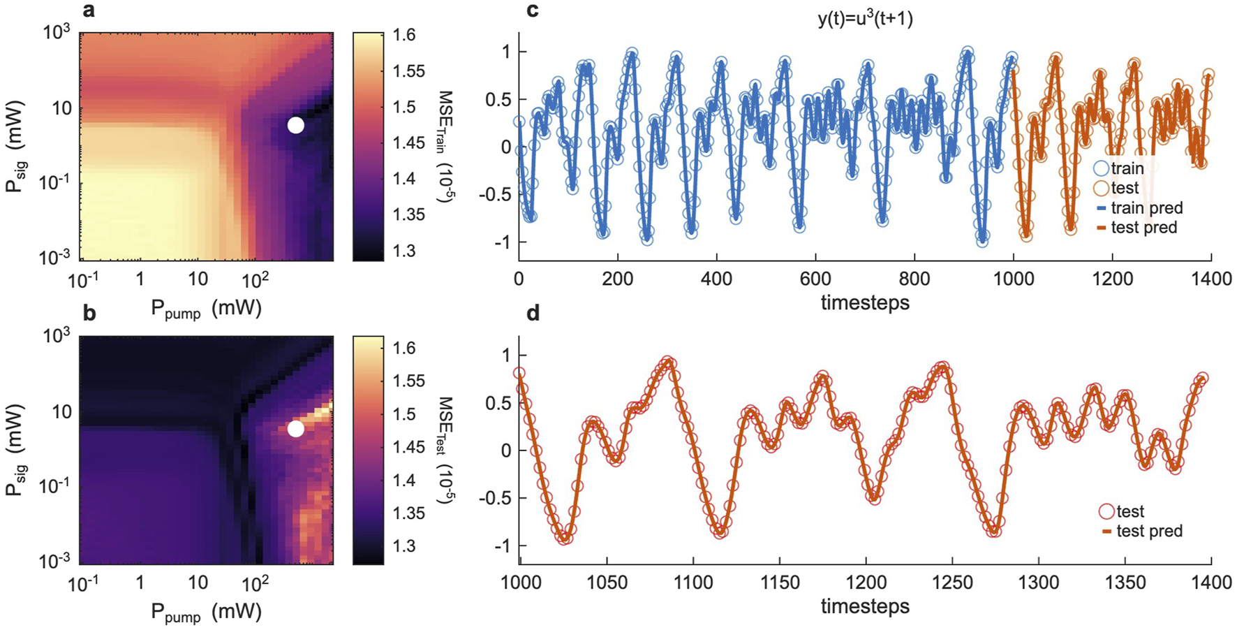
The results for $u(t_n)\to \mathrm{E}\mathrm{L}\mathrm{M}\to u^3(t_{n+1})$ are shown in Figure 6a,b, where we plot the MSE of the regression task associated with the nonlinear function of the Mackey-Glass time series, as obtained through ridge regression. The results show that the system can achieve an MSE of about $3\times 10^{-5}$ for both the training and testing sets, indicating that the system can effectively learn the underlying structure of the data and generalise to unseen samples. Similarly to the previous case, the training and test datasets (blue and orange squares) are shown in Figures 6c,d, along with the predicted training and testing time-series (blue and orange lines). Our results show that when trained to predict a nonlinear function of the time series, the reservoir still finds an optimal regime and can learn the task, but with higher overall error and a narrower optimal window. This parallels our regression findings: increasing the task complexity (here by a nonlinear transformation) demands greater reservoir complexity and pushes the system closer to its limits. We stress here that, in close comparison with Ref. (Jaurigue et al., 2025), our results correspond to a non-autonomous prediction task, where the ground-truth time-series is fed as an input during both the training and testing phases. In this scenario, with the inclusion of delay embedding on the readout matrix, the prediction task is effectively recast into a regression one (McCaul et al., 2025b). Our non-autonomous prediction results are quantitatively consistent with our recent observations in analysing quantum RC systems based on Rydberg atoms (McCaul et al., 2025b), since the variance of the ground-truth data amounts to 0.2209 for the case in Figure 5 0.008 for the case in Figure 6.

Figure 6

Figure 6. Non-autonomous time-series prediction, nonlinear case. (a,b) Training (a) and Testing (b) MSE error for the task $u(t_n)\to u^3(t_{n+1})$ as a function of the signal $P_s$ and pump $P_p$ powers. The MSE is plotted on a logarithmic scale (i.e., ${\mathrm{l}\mathrm{o}\mathrm{g}}_{10}MSE$). The white dot corresponds to the prediction results shown in (c,d). (c) Full Mackey-Glass time-series target for the training (blue crosses) and testing (orange crosses) datasets, superimposed on the reservoir prediction (blue and orange lines, respectively). The ground-truth target (cross markers) is plotted every 3 data points for visualisation purposes. (d) Same as (c), but illustrating only the testing dataset. Predicted values correspond to the blue line, while red crosses denote ground-truth targets.

4 Discussion

In summary, across all tasks – static function approximation, binary classification, and temporal prediction – the reservoir consistently performs best in an intermediate regime of operation. Specifically, configurations with moderate gain and high sensitivity (near the gain threshold) yield the lowest errors, whereas too little nonlinearity (low power) or excessive nonlinearity (deep into gain saturation) degrade performance. This robust trend suggests an underlying principle governing optimal reservoir performance, which we explore next by analysing the system’s expressivity and complexity.

4.1 Readout analysis: linear algebra properties

At the core of our photonic reservoir lies the combination of controllable nonlinear transformations and separability enabled by the internal dynamics of the multimode fibre. The physical properties of the transformation directly map into the readout matrix $\mathbf{H}$ employed as the design matrix of the ridge regression in Equation 3. As such, it is useful to analyse the standard linear algebraic metrics associated with the regularised linear regression problem $\mathbf{y}=\mathbf{W}\mathbf{H}$. In Figures 7a–c, we show the rank (Axler, 2015) of the readout matrix $\mathbf{H}$ for the three different tasks discussed in the previous section. All of these matrices have a number of rows corresponding to the number of pixels $(N=900)$ and a number of columns corresponding to the number of samples in the training set (included in the title of each subplot). As a rule of thumb reminder, it is expected that the best-performing configurations for the linear regression in Equation 3 should correspond to regions of the parameter space where the rank of the design matrix is maximised (Hastie et al., 2009). Comparing Figures 7a–c, it can be easily seen that our analysis is in good agreement with this intuitive consideration.

Figure 7

Figure 7. Linear Algebra metrics of the readout matrix $\mathbf{H}$. (a–c) Matrix rank of the readout matrix $\mathbf{H}$ as a function of the signal $P_s$ and pump $P_p$ powers for the regression (a), classification (b), and time-series prediction (c) tasks. The size of the readout matrix is $N\times M_{\text{train}}$. The number of training samples, included in the title of each panel, corresponds to $M_{\text{train}}=500$ for the regression task, $M_{\text{train}}=400$ for the spiral classification, and $M_{\text{train}}=1000$ for the time-series prediction. The number of features (pixels) in all cases is $N=900$. (d–f) Effective degrees of freedom $(edf)$ of the readout matrix $\mathbf{H}$ as a function of the signal $P_s$ and pump $P_p$ powers for the regression (d), classification (e), and time-series prediction (f) tasks. The $edf$ is defined in Equation 17, and we fixed the regression coefficient to $\lambda =10^{-4}$ for all cases and tasks.

In the presence of ridge regularisation, however, the inclusion of a penalisation term automatically forces the rank of the matrices to be near maximal, as even near-singular directions in $H$ can be inverted (at the cost of a penalty). This means that the true rank of the matrix to be inverted is effectively full at the matrix-inversion stage in most cases. A more suitable metric to analyse the expressivity of the design matrix is provided by the effective degrees of freedom $(edf)$ of $\mathbf{H}$, defined as (Hastie, 2020):

$edf\left(\mathbf{H},\lambda \right)={\displaystyle \sum _n}\frac{{\sigma }_n^2}{{\sigma }_n^2+\lambda },(17)$

where ${\sigma }_n$ are the singular values of $\mathbf{H}$. As suggested by the name, $edf(\mathbf{H},\lambda )$ provides a quantitative estimation of the number of singular values above the ridge regularisation threshold, namely, ${\sigma }_n>\sqrt{\lambda }=10^{-8}$. Different from the rank, which measures the number of independent columns or rows in the matrix, $edf$ measures the number of effective dimensions carrying meaningful information in the design matrix before readout training. The results for our three learning tasks are shown in Figures 7d–f. For each task, we also computed additional metrics, including the conditioning number, the average Shannon entropy of the readout matrix, and the average sample Shannon entropy. These results are included in Supplementary Figures S6–S8.

In summary, the matrix rank reveals how well $H$ can span the output space (flagging very poor configurations such as extremely lossy regimes). However, once the reservoir enters the nonlinear regime, even chaotic/random features can make $H$ full-rank, which improves training fit but not necessarily generalisation. The $edf$ provides a finer view by counting only the active dimensions given $\lambda$. We find that as the $edf$ increases, the model can fit more complex relations, and typically, performance improves, up to a point. Beyond that point, extra degrees of freedom confer no benefit and may even hurt generalisation.

The trade-off can be clearly appreciated by comparing our analysis to the prediction results for each task (cf. Figures 3–6). For the $\mathrm{s}\mathrm{i}\mathrm{n}\mathrm{c}$ task, we observed that training and testing MSE were consistent across the different signal and pump powers, suggesting minimal overfitting. This is reflected in both high rank and $edf$ across both regions. In the case of time-series prediction, both the rank and $edf$ follow the same trend as the nonlinear regression scenario, as the two tasks (before setting a target) essentially match (generating a set of nonlinear features out of a one-dimensional dataset). For the classification case, conversely, the MSE analysis suggested strong overfitting in the highly nonlinear regime. In this case, the rank is nearly maximised across the high sensitivity and high nonlinearity regions, but the $edf$ is remarkably high for the latter. This is a clear indication that the reservoir is generating a large number of nonlinear features, but most of these are too chaotic to contribute to effective generalisation. Here, the reservoir manifests optimal performance in the high-sensitivity region, which is to be expected for a challenging classification task requiring nonlinear separability.

4.2 The role of complexity

In RC, learning occurs only after propagation in the reservoir via linear regression, and the task target is never part of the encoding and processing. As shown in our results, in fact, an identical reservoir readout can accommodate different tasks, suggesting that successful computations not only originate from intrinsic properties of the readout (or design) matrix $\mathbf{H}$, but also on its ability to generate structured features of the input data that can be adapted across a wide range of target functions. In essence, expressivity in our photonic reservoir is not just a linear algebra property; on the contrary, we need to assess how much information is generated from the input to the hidden layer and what structure the reservoir and embedding layers impose on it. In a physical RC system, these properties will derive from the physical transformation that originates from the system’s evolution. Said differently, information is encoded and transformed in a way that optimises the amount of information exposed at the readout of the reservoir, and our system is particularly suitable for assessing the information content of the readout matrix across different nonlinear regimes for the three types of tasks under consideration.

Linear algebraic metrics such as rank, conditioning, and effective degrees of freedom provide valuable but incomplete insights into the reservoir computational performance, and they mainly offer guidance on the ability of the system to fit the training data and do not fully capture the underlying dynamical complexity that dictates performance in nonlinear tasks. To address this limitation, we analysed the reservoir output using algorithmic complexity, expressed by the Kolmogorov Complexity (KC), which measures the structured complexity or regularity of the reservoir-generated features.

The KC measures the algorithmic randomness of a string of bits, which is informally defined as the length of the shortest program that can produce that specific string of bits. While a unique definition of KC is not readily available, several approaches have been proposed, which are mostly dependent on the type of data under consideration. Following recent results in the analysis of pattern formation in nonlinear photonic systems (Perego et al., 2022), we approximate the KC of our reservoir processing via the Lempel–Ziv algorithm as implemented by Kaspar and Schuster (Kaspar and Schuster, 1987).

In this approach, the value of each output pixel is binarised relative to its mean (1 above mean and 0 otherwise), and the resulting binary pattern is analysed for compressibility. This initial complexity count is then normalised by the complexity of a random binary pattern of the same size $(N/{\log }_2(N))$, so that KC = 1 corresponds to a maximally random (incompressible) output distribution by definition. Consequently, any KC value below 1, denoted as “sub-unity” KC in Ref (Kaspar and Schuster, 1987), indicates the presence of some underlying order or redundancy in the reservoir outputs. In this case, the output patterns are not purely random but contain structure that makes them algorithmically compressible.

We compute two different versions of the KC following the procedures detailed in Supplementary Section S4. If the mean is computed across the sample space (average the value of the pixel across all samples), we are computing the feature KC. If the mean is computed across the feature space (average the value of the pixel across all pixels for a given sample), we obtain the sample KC. In brief, sample KC characterises complexity across spatial features (pixels) for each individual reservoir output (sample), whereas feature KC measures complexity across samples for each spatial feature (pixel). Here, we primarily focus on sample KC as it directly captures how structured (compressible) or random (incompressible) each reservoir output pattern is, and thus correlates closely with the quality of reservoir transformations relevant for task performance. The results for the sample KC are shown in Figure 8, while the feature KC plots are in Supplementary Figure S9.

Figure 8

Figure 8. Sample Kolmogorov Complexity (KC) of the readout matrix $\mathbf{H}$. (a–c) Average sample KC of the readout matrix $\mathbf{H}$ as a function of the signal $P_s$ and pump $P_p$ powers for the regression (a), classification (b), and time-series prediction (c) tasks. For each combination $(P_s,P_p)$, the sample KC is computed for each CCD output and then averaged across all samples. (d–f) Relative variability of sample KC across the dataset as a function of the signal $P_s$ and pump $P_p$ powers for the regression (d), classification (e), and time-series prediction (f) tasks. The relative variability is the ratio of the standard deviation associated with each average in (a–c) divided by the corresponding average.

Figures 8a–c illustrate the normalised sample KC averaged across all samples, computed as a function of pump and signal powers for each computational task. A clear and consistent pattern emerges: in regimes of low optical power, the KC values are substantially below unity, indicating highly structured (overly regular) reservoir responses. This aligns with poor task performance due to insufficient nonlinearity in the reservoir transformations. Conversely, in regimes of excessively high pump and signal power—corresponding to chaotic or strongly saturated dynamics—the KC approaches unity, reflecting output patterns that resemble random noise. Such randomness provides high expressivity but limits generalisation, resulting in suboptimal task accuracy. To quantify the KC variability across samples, we also compute the standard deviation of the KC values (Figures 8d–f). The standard deviation is normalised by the mean KC value to provide a relative measure of variability. This analysis reveals that the KC variability is significantly lower in the optimal regime, indicating that the reservoir outputs are not only structured but also exhibit consistent patterns across samples.

It is important to note that KC is a finer measure of order/disorder than simple statistical metrics. Kolmogorov algorithmic complexity can detect the emergence of subtle structures in high-dimensional nonlinear systems that other measures might miss. For instance, a binary output pattern might have high Shannon entropy (each pixel is 0/1 50% of the time) but still be highly structured (e.g., repeated patterns), yielding a KC well below 1. The sub-unity KC captures this hidden regularity, whereas an entropy measure could mistakenly suggest “maximal randomness.” Essentially, KC$<1$ indicates that the reservoir outputs exhibit inherent structure or redundancy beyond random noise, reflecting the reservoir’s dynamics on the output distribution.

In this context, the KC provides a metric that is closer to the spectral radius or Lyapunov coefficients in time-series analysis and time-dependent reservoir systems ruled by ordinary differential equations (Li and Vitányi, 2019). In echo state networks, for instance, the spectral radius of the reservoir matrix needs to be carefully tuned to balance stability and chaos (Lukoševičius et al., 2012). Here, the KC of the outputs serves a similar role: it quantitatively reflects where our system lies on the spectrum from linear, nonlinear, and chaotic. Specifically, KC$\ll 1$ corresponds to an overly stable/linear regime (too much order), KC $\sim 1$ corresponds to a chaotic regime (output is effectively random), and intermediate KC indicates a complex but learnable regime, which is exactly where we see optimal computational performance across all our tasks. This deep connection between performance and output complexity provides a quantitative underpinning to the oft-mentioned ‘optimal balance’ or task-dependent sweet spot in reservoir computing (e.g., as observed in spin-wave reservoirs (Gartside et al., 2022; Lee et al., 2024)).

5 Conclusion

In this work, we tackle the challenge of nonlinear tunability in photonic reservoir computing by designing a single system that can adapt its nonlinearity and complexity to different tasks. Using gain-controlled multimode fibre and wavefront encoding, we demonstrated that simply adjusting pump and signal powers provides such tunability, effectively reconfiguring the nonlinear operating regime of the reservoir on demand. Through simulations on regression, classification, and time-series benchmarks, we found a consistent trend: an intermediate regime near the gain threshold yields optimal performance, whereas regimes that are too linear or overly nonlinear underperform. A central contribution of this work is linking the reservoir computing performance to the Kolmogorov complexity of its outputs. We showed that in the optimal regime, the reservoir generates outputs with high algorithmic structure, detectable as a sub-unity Kolmogorov complexity, indicating maximal exploitation of nonlinear dynamics to produce informative features. Conventional metrics (including rank, effective degrees of freedom, and condition number) alone could not fully explain the learning performance in the nonlinear regime, whereas the complexity measure provided critical insight into why the ‘just-right’ amount of chaos is best. Unlike conventional metrics, in fact, the KC assesses the reservoir’s intrinsic output diversity: since the reservoir is not trained toward any one task while processing the dataset, it should produce a wealth of structured input transformations so that the linear readout can adapt to any required function. In summary, all metrics are important pieces of the puzzle: rank, conditioning, and $edf$ are essential to understanding the fitting capabilities of the system, while the KC provides key insights to understand how the reservoir behaves once you’re in the nonlinear regime. Our findings suggest that complexity can serve as a design metric for neuromorphic photonics. By quantifying output complexity, one can objectively tune a photonic reservoir to its optimal state without exhaustive task-specific trials. In practice, this could guide the development of self-optimising photonic circuits that adjust their gain or nonlinearity in real-time to maintain maximal computational performance. Future work will explore implementing explicit feedback to tackle temporal tasks more naturally, and include the effects of ASE and experimental noise, although such analysis will likely require direct experimental implementation due to the computational costs associated with more involved modelling of the multimode fibre dynamics. In this context, key experimental challenges are likely related to the stability of the multimode fibre across the dataset processing, as mechanical perturbations and bending can affect the linear (and potentially, nonlinear) coupling of the MMF modes and introduce dynamical changes in the transmission matrix of the system (Shekel et al., 2024). In the presence of gain media, however, preliminary experimental results suggest that nonlinear wavefront control is achievable in practice (Sperber et al., 2020). Overall, our work demonstrates that harnessing and optimising complexity is a viable pathway to significantly improve photonic reservoir computing performance, paving the way for adaptive, task-flexible optical data processors.

Data availability statement

The datasets presented in this study can be found in online repositories. The names of the repository/repositories and accession number(s) can be found below: https://doi.org/10.17028/rd.lboro.29482847. Numerical codes are available from the corresponding author upon reasonable request.

Author contributions

GM: Conceptualization, Methodology, Resources, Supervision, Writing – original draft, Writing – review and editing. LO: Writing – review and editing, Software, Visualization. JT: Data curation, Software, Visualization, Writing – review and editing, Conceptualization, Formal Analysis, Funding acquisition, Investigation, Methodology, Project administration, Resources, Supervision, Validation, Writing – original draft.

Funding

The author(s) declare that financial support was received for the research and/or publication of this article. This work was supported by the UK Engineering and Physical Sciences Research Council (EPSRC, Grant number EP/W028344/1), the UK Research and Innovation (UKRI) Horizon Europe guarantee scheme for the QRC-4-ESP project (Grant number 10108296), the European Union and the European Innovation Council through the Horizon Europe project QRC-4-ESP (Grant Agreement no. 101129663). LO acknowledges support from The Leverhulme Trust (Leverhulme Early Career Fellowship ECF-2023-315). Sulis is funded by EPSRC Grant EP/T022108/1 and the HPC Midlands+ consortium.

Acknowledgments

This paper acknowledges the use of the Lovelace HPC service at Loughborough University. Calculations were also performed using the Sulis Tier 2 HPC platform hosted by the Scientific Computing Research Technology Platform at the University of Warwick. We thank Dr Maxwell Rowley for discussions on the gain dynamics in fibre systems and Dr Gerard McCaul for insightful discussions on the Kolmogorov Complexity analysis and interpretation.

Conflict of interest

Author GM was employed by LumiAIres Ltd.

The remaining authors declare that the research was conducted in the absence of any commercial or financial relationships that could be construed as a potential conflict of interest.

Generative AI statement

The author(s) declare that no Generative AI was used in the creation of this manuscript.

Publisher’s note

All claims expressed in this article are solely those of the authors and do not necessarily represent those of their affiliated organizations, or those of the publisher, the editors and the reviewers. Any product that may be evaluated in this article, or claim that may be made by its manufacturer, is not guaranteed or endorsed by the publisher.

Supplementary material

The Supplementary Material for this article can be found online at: https://www.frontiersin.org/articles/10.3389/fnano.2025.1631564/full#supplementary-material

References

Agrawal, G. P., and Premaratne, M. (2011). Light propagation in gain Media_Optical amplifiers. Cambridge University Press.

Google Scholar

Amodei, D., Hernandez, D., Sastry, G., Clark, J., Brockman, G., and Sutskever, I. (2018). AI and compute. Available online at: https://openai.com/research/ai-and-compute.Tech.rep.,OpenAI.

Google Scholar

Appeltant, L., Soriano, M. C., Van der Sande, G., Danckaert, J., Massar, S., Dambre, J., et al. (2011). Information processing using a single dynamical node as complex system. Nat. Commun. 2, 468. doi:10.1038/ncomms1476

PubMed Abstract | CrossRef Full Text | Google Scholar

Axler, S. (2015). “Linear algebra done right,” in Undergraduate texts in mathematics. Cham: Springer International Publishing. doi:10.1007/978-3-319-11080-6

CrossRef Full Text | Google Scholar

Bertschinger, N., and Natschläger, T. (2004). Real-time computation at the edge of chaos in recurrent neural networks. Neural Comput. 16, 1413–1436. doi:10.1162/089976604323057443

PubMed Abstract | CrossRef Full Text | Google Scholar

Bhardwaj, E., Alexander, R., and Becker, C. (2025). Limits to AI growth: the ecological and social consequences of scaling. arXiv. doi:10.48550/arXiv.2501.17980

CrossRef Full Text | Google Scholar

Brunner, D., Shastri, B. J., Qadasi, M. A. A., Ballani, H., Barbay, S., Biasi, S., et al. (2025). Roadmap on neuromorphic photonics. arXiv. doi:10.48550/arXiv.2501.07917

CrossRef Full Text | Google Scholar

Buck, J. A. (2004). Fundamentals of optical fibers. Wiley series in pure and applied optics (Hoboken, NJ: Wiley-Interscience), 2.

Google Scholar

Dale, M., Dewhirst, J., O’Keefe, S., Sebald, A., Stepney, S., and Trefzer, M. A. (2019). “The role of structure and complexity on reservoir computing quality,” in Unconventional computation and natural computation. Editors I. McQuillan, and S. Seki (Cham: Springer International Publishing), 11493, 52–64. doi:10.1007/978-3-030-19311-9_6

CrossRef Full Text | Google Scholar

Dong, H., Jaurigue, L., and Lüdge, K. (2025). Time-multiplexed reservoir computing with quantum-dot lasers: impact of charge-carrier scattering timescale. Phys. status solidi (RRL) – Rapid Res. Lett. 19, 2400433. doi:10.1002/pssr.202400433

CrossRef Full Text | Google Scholar

Dong, J., Ohana, R., Rafayelyan, M., and Krzakala, F. (2020b). Reservoir computing meets recurrent kernels and structured transforms. arXiv:2006.07310 cs, eess, Stat. doi:10.48550/arXiv.2006.07310

CrossRef Full Text | Google Scholar

Dong, J., Rafayelyan, M., Krzakala, F., and Gigan, S. (2020a). Optical reservoir computing using multiple light scattering for chaotic systems prediction. IEEE J. Sel. Top. Quantum Electron. 26, 1–12. doi:10.1109/JSTQE.2019.2936281

CrossRef Full Text | Google Scholar

Farhat, N. H., Psaltis, D., Prata, A., and Paek, E. (1985). Optical implementation of the Hopfield model. Appl. Opt. 24, 1469. doi:10.1364/AO.24.001469

PubMed Abstract | CrossRef Full Text | Google Scholar

Florentin, R., Kermene, V., Benoist, J., Desfarges-Berthelemot, A., Pagnoux, D., Barthélémy, A., et al. (2017). Shaping the light amplified in a multimode fiber. Light Sci. and Appl. 6, e16208. doi:10.1038/lsa.2016.208

PubMed Abstract | CrossRef Full Text | Google Scholar

Gallicchio, C., and Micheli, A. (2017). Echo state property of deep reservoir computing networks. Cogn. Comput. 9, 337–350. doi:10.1007/s12559-017-9461-9

CrossRef Full Text | Google Scholar

Gartside, J. C., Stenning, K. D., Vanstone, A., Holder, H. H., Arroo, D. M., Dion, T., et al. (2022). Reconfigurable training and reservoir computing in an artificial spin-vortex ice via spin-wave fingerprinting. Nat. Nanotechnol. 17, 460–469. doi:10.1038/s41565-022-01091-7

PubMed Abstract | CrossRef Full Text | Google Scholar

Ghosh, S., Opala, A., Matuszewski, M., Paterek, T., and Liew, T. C. H. (2019). Quantum reservoir processing. npj Quantum Inf. 5, 35. doi:10.1038/s41534-019-0149-8

CrossRef Full Text | Google Scholar

Gigan, S. (2022). Imaging and computing with disorder. Nat. Phys. 18, 980–985. doi:10.1038/s41567-022-01681-1

CrossRef Full Text | Google Scholar

Goldmann, M., Köster, F., Lüdge, K., and Yanchuk, S. (2020). Deep time-delay reservoir computing: dynamics and memory capacity. Chaos An Interdiscip. J. Nonlinear Sci. 30, 093124. doi:10.1063/5.0017974

PubMed Abstract | CrossRef Full Text | Google Scholar

Haken, H., and Sauermann, H. (1963). Nonlinear interaction of laser modes. Z. für Phys. 173, 261–275. doi:10.1007/BF01377828

CrossRef Full Text | Google Scholar

Hary, M., Brunner, D., Leybov, L., Ryczkowski, P., Dudley, J. M., and Genty, G. (2025). Principles and metrics of extreme learning machines using a highly nonlinear fiber. Nanophotonics. doi:10.1515/nanoph-2025-0012

PubMed Abstract | CrossRef Full Text | Google Scholar

Hastie, T. (2020). Ridge regularization: an essential concept in data science. Technometrics 62, 426–433. doi:10.1080/00401706.2020.1791959

PubMed Abstract | CrossRef Full Text | Google Scholar

Hastie, T., Tibshirani, R., and Friedman, J. (2009). The elements of statistical learning: data mining, inference, and prediction. Springer.

Google Scholar

Hurtado, A., Romeira, B., Buckley, S., Cheng, Z., and Shastri, B. J. (2022). Emerging optical materials, devices and systems for photonic neuromorphic computing: introduction to special issue. Opt. Mater. Express 12, 4328. doi:10.1364/OME.477577

CrossRef Full Text | Google Scholar

Jaeger, H., and Haas, H. (2004). Harnessing nonlinearity: predicting chaotic systems and saving energy in wireless communication. Science 304, 78–80. doi:10.1126/science.1091277

PubMed Abstract | CrossRef Full Text | Google Scholar

Jaurigue, J., Robertson, J., Hurtado, A., Jaurigue, L., and Lüdge, K. (2025). Post-processing methods for delay embedding and feature scaling of reservoir computers. Commun. Eng. 4, 10–13. doi:10.1038/s44172-024-00330-0

PubMed Abstract | CrossRef Full Text | Google Scholar

Jiménez-González, P., Soriano, M. C., and Lacasa, L. (2025). Leveraging chaos in the training of artificial neural networks. arXiv, 2506. doi:10.48550/arXiv.2506.08523

CrossRef Full Text | Google Scholar

Jumper, J., Evans, R., Pritzel, A., Green, T., Figurnov, M., Ronneberger, O., et al. (2021). Highly accurate protein structure prediction with AlphaFold. Nature 596, 583–589. doi:10.1038/s41586-021-03819-2

PubMed Abstract | CrossRef Full Text | Google Scholar

Kaspar, F., and Schuster, H. G. (1987). Easily calculable measure for the complexity of spatiotemporal patterns. Phys. Rev. A 36, 842–848. doi:10.1103/PhysRevA.36.842

PubMed Abstract | CrossRef Full Text | Google Scholar

Kesgin, B. U., and Tegin, U. (2025). Photonic neural networks at the edge of spatiotemporal chaos in multimode fibers. Nanophotonics. doi:10.1515/nanoph-2024-0593

PubMed Abstract | CrossRef Full Text | Google Scholar

Kudithipudi, D., Schuman, C., Vineyard, C. M., Pandit, T., Merkel, C., Kubendran, R., et al. (2025). Neuromorphic computing at scale. Nature 637, 801–812. doi:10.1038/s41586-024-08253-8

PubMed Abstract | CrossRef Full Text | Google Scholar

Lee, O., Wei, T., Stenning, K. D., Gartside, J. C., Prestwood, D., Seki, S., et al. (2024). Task-adaptive physical reservoir computing. Nat. Mater. 23, 79–87. doi:10.1038/s41563-023-01698-8

PubMed Abstract | CrossRef Full Text | Google Scholar

Legenstein, R., and Maass, W. (2007). Edge of chaos and prediction of computational performance for neural circuit models. Neural Netw. 20, 323–334. doi:10.1016/j.neunet.2007.04.017

PubMed Abstract | CrossRef Full Text | Google Scholar

Li, M., and Vitányi, P. (2019). “An introduction to Kolmogorov complexity and its applications,” in Texts in computer science. Cham: Springer International Publishing. doi:10.1007/978-3-030-11298-1

CrossRef Full Text | Google Scholar

Lukoševičius, M. (2012). “A practical guide to applying echo state networks,” in Neural networks: tricks of the trade. Editors G. Montavon, G. B. Orr, and K. R. Müller (Berlin, Heidelberg: Springer Berlin Heidelberg), 7700, 659–686. doi:10.1007/978-3-642-35289-8_36

CrossRef Full Text | Google Scholar

Maass, W. (2011). Liquid state machines: motivation, theory, and applications. World Sci., 275–296. doi:10.1142/9781848162778_0008

CrossRef Full Text | Google Scholar

Maass, W., Joshi, P., and Sontag, E. D. (2007). Computational aspects of feedback in neural circuits. PLOS Comput. Biol. 3, e165. doi:10.1371/journal.pcbi.0020165

PubMed Abstract | CrossRef Full Text | Google Scholar

Maass, W., Natschläger, T., and Markram, H. (2002). Real-time computing without stable states: a new framework for neural computation based on perturbations. Neural Comput. 14, 2531–2560. doi:10.1162/089976602760407955

PubMed Abstract | CrossRef Full Text | Google Scholar

Marcucci, G., Pierangeli, D., and Conti, C. (2020). Theory of neuromorphic computing by waves: machine learning by rogue waves, dispersive shocks, and solitons. Phys. Rev. Lett. 125, 093901. doi:10.1103/PhysRevLett.125.093901

PubMed Abstract | CrossRef Full Text | Google Scholar

Marković, D., Mizrahi, A., Querlioz, D., and Grollier, J. (2020). Physics for neuromorphic computing. Nat. Rev. Phys. 2, 499–510. doi:10.1038/s42254-020-0208-2

CrossRef Full Text | Google Scholar

McCaul, G., Jacobs, K., and Bondar, D. I. (2023). Towards single atom computing via high harmonic generation. Eur. Phys. J. Plus 138, 123. doi:10.1140/epjp/s13360-023-03649-3

CrossRef Full Text | Google Scholar

McCaul, G., Totero Gongora, J. S., Otieno, W., Savelev, S., Zagoskin, A., and Balanov, A. G. (2025b). Minimal quantum reservoirs with Hamiltonian encoding. arXiv:2505.22575. doi:10.48550/arXiv.2505.22575

CrossRef Full Text | Google Scholar

McCaul, G., Tripathy, G., Marcucci, G., and Totero Gongora, J. S. (2025a). Unwrapping photonic reservoirs: enhanced expressivity via random fourier encoding over stretched domains. arXiv:2506.01410. doi:10.48550/arXiv.2506.01410

CrossRef Full Text | Google Scholar

McMahon, P. L. (2023). The physics of optical computing. Nat. Rev. Phys. 5, 717–734. doi:10.1038/s42254-023-00645-5

CrossRef Full Text | Google Scholar

Merolla, P. A., Arthur, J. V., Alvarez-Icaza, R., Cassidy, A. S., Sawada, J., Akopyan, F., et al. (2014). A million spiking-neuron integrated circuit with a scalable communication network and interface. Science 345, 668–673. doi:10.1126/science.1254642

PubMed Abstract | CrossRef Full Text | Google Scholar

Nerenberg, S., Neill, O. D., Marcucci, G., and Faccio, D. (2025). Photon number-resolving quantum reservoir computing. Opt. Quantum 3, 201–210. doi:10.1364/OPTICAQ.553294

CrossRef Full Text | Google Scholar

Ng, W. K., Dranczewski, J., Fischer, A., Raziman, T. V., Saxena, D., Farchy, T., et al. (2024). Retinomorphic machine vision in a network laser. arXiv:2407.15558. doi:10.48550/arXiv.2407.15558

CrossRef Full Text | Google Scholar

Olivieri, L., Cooper, A. R., Peters, L., Cecconi, V., Pasquazi, A., Peccianti, M., et al. (2025). Adiabatic energetic annealing via dual single-pixel detection in an optical nonlinear ising machine. ACS Photonics 12, 2896–2901. doi:10.1021/acsphotonics.4c02496

PubMed Abstract | CrossRef Full Text | Google Scholar

Owen-Newns, D., Jaurigue, L., Robertson, J., Adair, A., Jaurigue, J. A., Lüdge, K., et al. (2025). Photonic spiking neural network built with a single VCSEL for high-speed time series prediction. Commun. Phys. 8, 110–119. doi:10.1038/s42005-025-02000-9

CrossRef Full Text | Google Scholar

Perego, A. M., Bessin, F., and Mussot, A. (2022). Complexity of modulation instability. Phys. Rev. Res. 4, L022057. doi:10.1103/PhysRevResearch.4.L022057

CrossRef Full Text | Google Scholar

Pierangeli, D., Marcucci, G., and Conti, C. (2021). Photonic extreme learning machine by free-space optical propagation. Photonics Res. 9, 1446–1454. doi:10.1364/PRJ.423531

CrossRef Full Text | Google Scholar

Pierangeli, D., Palmieri, V., Marcucci, G., Moriconi, C., Perini, G., De Spirito, M., et al. (2020). Living optical random neural network with three dimensional tumor spheroids for cancer morphodynamics. Commun. Phys. 3, 160–10. doi:10.1038/s42005-020-00428-9

CrossRef Full Text | Google Scholar

Pierro, A., Heiney, K., Shrivastava, S., Marcucci, G., and Nichele, S. (2023). Optimization of a hydrodynamic computational reservoir through evolution. Proc. Genet. Evol. Comput. Conf. 23, 202–210. doi:10.1145/3583131.3590355

CrossRef Full Text | Google Scholar

Psaltis, D., and Farhat, N. (1985). Optical information processing based on an associative-memory model of neural nets with thresholding and feedback. Opt. Lett. 10, 98. doi:10.1364/OL.10.000098

PubMed Abstract | CrossRef Full Text | Google Scholar

Rafayelyan, M., Dong, J., Tan, Y., Krzakala, F., and Gigan, S. (2020). Large-scale optical reservoir computing for spatiotemporal chaotic systems prediction, Phys. Rev. X 10, 041037. doi:10.1103/PhysRevX.10.041037

CrossRef Full Text | Google Scholar

Rahmani, B., Oguz, I., Tegin, U., Hsieh, Jl, Psaltis, D., and Moser, C. (2022). Learning to image and compute with multimode optical fibers. Nanophotonics 11, 1071–1082. doi:10.1515/nanoph-2021-0601

PubMed Abstract | CrossRef Full Text | Google Scholar

Robertson, J., Hejda, M., Bueno, J., and Hurtado, A. (2020). Ultrafast optical integration and pattern classification for neuromorphic photonics based on spiking VCSEL neurons. Sci. Rep. 10, 6098. doi:10.1038/s41598-020-62945-5

PubMed Abstract | CrossRef Full Text | Google Scholar

Rowley, M., Hanzard, P. H., Cutrona, A., Bao, H., Chu, S. T., Little, B. E., et al. (2022). Self-emergence of robust solitons in a microcavity. Nature 608, 303–309. doi:10.1038/s41586-022-04957-x

PubMed Abstract | CrossRef Full Text | Google Scholar

Roy, K., Jaiswal, A., and Panda, P. (2019). Towards spike-based machine intelligence with neuromorphic computing. Nature 575, 607–617. doi:10.1038/s41586-019-1677-2

PubMed Abstract | CrossRef Full Text | Google Scholar

Saeed, S., Müftüoglu, M., Cheeran, G. R., Bocklitz, T., Fischer, B., and Chemnitz, M. (2025). Nonlinear inference capacity of fiber-optical extreme learning machines. ArXiv:2501.18894 [physics] [Preprint]. doi:10.48550/arXiv.2501.18894

CrossRef Full Text | Google Scholar

Shastri, B. J., Tait, A. N., Ferreira de Lima, T., Pernice, W. H. P., Bhaskaran, H., Wright, C. D., et al. (2021). Photonics for artificial intelligence and neuromorphic computing. Nat. Photonics 15, 102–114. doi:10.1038/s41566-020-00754-y

CrossRef Full Text | Google Scholar

Shekel, R., Sulimany, K., Resisi, S., Finkelstein, Z., Lib, O., Popoff, S. M., et al. (2024). Tutorial: how to build and control an all-fiber wavefront modulator using mechanical perturbations. J. Phys. Photonics 6, 033002. doi:10.1088/2515-7647/ad5774

CrossRef Full Text | Google Scholar

Shishavan, N. S., Manuylovich, E., Kamalian-Kopae, M., and Perego, A. M. (2025). Optical neuromorphic computing based on chaotic frequency combs in nonlinear microresonators. arXiv:2501.17113. doi:10.48550/arXiv.2501.17113

CrossRef Full Text | Google Scholar

Skalli, A., Sunada, S., Goldmann, M., Gebski, M., Reitzenstein, S., Lott, J. A., et al. (2025). Model-free front-to-end training of a large high performance laser neural network. arXiv:2503.16943. doi:10.48550/arXiv.2503.16943

CrossRef Full Text | Google Scholar

Sperber, T., Billault, V., Dussardier, B., Gigan, S., and Sebbah, P. (2020). Gain as configurable disorder-adaptive pumping for control of multimode fiber amplifiers and lasers. arXiv:2008.04085 Phys. doi:10.48550/arXiv.2008.04085

CrossRef Full Text | Google Scholar

Sperber, T., Billault, V., Sebbah, P., and Gigan, S. (2019). Wavefront shaping of the pump in multimode fiber amplifiers; the gain-dependent transmission matrix. arXiv:1911.07812 Phys. doi:10.48550/arXiv.1911.07812

CrossRef Full Text | Google Scholar

Stone, A. D., Tureci, H. E., and Schwefel, H. G. (2005). Mode competition and output power from regular and chaotic dielectric cavity lasers. Front. Opt. (Tucson, Ariz. OSA), FWQ1. doi:10.1364/FIO.2005.FWQ1

CrossRef Full Text | Google Scholar

Talukder, R., Skalli, A., Porte, X., Thorpe, S., and Brunner, D. (2025). A spiking photonic neural network of 40000 neurons, trained with latency and rank-order coding for leveraging sparsity. Neuromorphic Comput. Eng. 5, 034003. doi:10.1088/2634-4386/addee7

CrossRef Full Text | Google Scholar

Tanaka, G., Yamane, T., Héroux, J. B., Nakane, R., Kanazawa, N., Takeda, S., et al. (2019). Recent advances in physical reservoir computing: a review. Neural Netw. 115, 100–123. doi:10.1016/j.neunet.2019.03.005

PubMed Abstract | CrossRef Full Text | Google Scholar

Teğin, U., Yıldırım, M., Oğuz, İ., Moser, C., and Psaltis, D. (2021). Scalable optical learning operator. Nat. Comput. Sci. 1, 542–549. doi:10.1038/s43588-021-00112-0

PubMed Abstract | CrossRef Full Text | Google Scholar

Totero Gongora, J. S., Miroshnichenko, A. E., Kivshar, Y. S., and Fratalocchi, A. (2017). Anapole nanolasers for mode-locking and ultrafast pulse generation. Nat. Commun. 8, 15535. doi:10.1038/ncomms15535

PubMed Abstract | CrossRef Full Text | Google Scholar

Totero Gongora, J.S., Miroshnichenko, A.E., Kivshar, Y.S., and Fratalocchi, A. (2016), Energy equipartition and unidirectional emission in a spaser nanolaser. Laser and Photonics Reviews, 10: 432–440. doi:10.1002/lpor.201500239

CrossRef Full Text | Google Scholar

Trinel, J. B., Cocq, G. L., Quiquempois, Y., Andresen, E. R., Vanvincq, O., and Bigot, L. (2017). Theoretical study of gain-induced mode coupling and mode beating in few-mode optical fiber amplifiers. Opt. Express 25, 2377–2390. doi:10.1364/OE.25.002377

PubMed Abstract | CrossRef Full Text | Google Scholar

Valensise, C. M., Grecco, I., Pierangeli, D., and Conti, C. (2022). Large-scale photonic natural language processing. Photonics Res. 10, 2846–2853. doi:10.1364/PRJ.472932

CrossRef Full Text | Google Scholar

Wang, D., Nie, Y., Hu, G., Tsang, H. K., and Huang, C. (2024a). Ultrafast silicon photonic reservoir computing engine delivering over 200 TOPS. Nat. Commun. 15, 10841. doi:10.1038/s41467-024-55172-3

PubMed Abstract | CrossRef Full Text | Google Scholar

Wang, H., Hu, J., Baek, Y., Tsuchiyama, K., Joly, M., Liu, Q., et al. (2024c). Optical next generation reservoir computing. arXiv:2404.07857. doi:10.48550/arXiv.2404.07857

CrossRef Full Text | Google Scholar

Wang, H., Hu, J., Morandi, A., Nardi, A., Xia, F., Li, X., et al. (2024d). Large-scale photonic computing with nonlinear disordered media. Nat. Comput. Sci. 4, 429–439. doi:10.1038/s43588-024-00644-1

PubMed Abstract | CrossRef Full Text | Google Scholar

Wang, Z., Müller, K., Filipovich, M., Launay, J., Ohana, R., Pariente, G., et al. (2024b). Streamlined optical training of large-scale modern deep learning architectures with direct feedback alignment. arXiv:2409.12965. doi:10.48550/arXiv.2409.12965

CrossRef Full Text | Google Scholar

Wei, X., Jing, J. C., Shen, Y., and Wang, L. V. (2020). Harnessing a multi-dimensional fibre laser using genetic wavefront shaping. Light Sci. and Appl. 9, 149. doi:10.1038/s41377-020-00383-8

PubMed Abstract | CrossRef Full Text | Google Scholar

Xia, F., Kim, K., Eliezer, Y., Han, S., Shaughnessy, L., Gigan, S., et al. (2024). Nonlinear optical encoding enabled by recurrent linear scattering. Nat. Photonics 18, 1067–1075. doi:10.1038/s41566-024-01493-0

PubMed Abstract | CrossRef Full Text | Google Scholar

Xu, Z., Zhou, T., Ma, M., Deng, C., Dai, Q., and Fang, L. (2024). Large-scale photonic chiplet Taichi empowers 160-TOPS/W artificial general intelligence. Science 384, 202–209. doi:10.1126/science.adl1203

PubMed Abstract | CrossRef Full Text | Google Scholar