 Natalya A. Kramarova1*
 Jerald R. Ziemke2
 Liang-Kang Huang3
 Jay R. Herman4
 Krzysztof Wargan3,1
 Colin J. Seftor3
 Gordon J. Labow3
 Luke D. Oman1
- 1NASA Goddard Space Flight Center, Greenbelt, MD, United States
- 2Goddard Earth Sciences Technology and Research (GESTAR)/Morgan State University, Baltimore, MD, United States
- 3Science Systems and Applications, Inc. (SSAI), Lanham, MD, United States
- 4University of Maryland, Baltimore County, Baltimore, MD, United States
Discrete wavelength radiance measurements from the Deep Space Climate Observatory (DSCOVR) Earth Polychromatic Imaging Camera (EPIC) allows derivation of global synoptic maps of total and tropospheric ozone columns every hour during Northern Hemisphere (NH) Summer or 2 hours during Northern Hemisphere winter. In this study, we present version 3 retrieval of Earth Polychromatic Imaging Camera ozone that covers the period from June 2015 to the present with improved geolocation, calibration, and algorithmic updates. The accuracy of total and tropospheric ozone measurements from EPIC have been evaluated using correlative satellite and ground-based total and tropospheric ozone measurements at time scales from daily averages to monthly means. The comparisons show good agreement with increased differences at high latitudes. The agreement improves if we only accept retrievals derived from the EPIC 317 nm triplet and limit solar zenith and satellite looking angles to 70°. With such filtering in place, the comparisons of EPIC total column ozone retrievals with correlative satellite and ground-based data show mean differences within ±5-7 Dobson Units (or 1.5–2.5%). The biases with other satellite instruments tend to be mostly negative in the Southern Hemisphere while there are no clear latitudinal patterns in ground-based comparisons. Evaluation of the EPIC ozone time series at different ground-based stations with the correlative ground-based and satellite instruments and ozonesondes demonstrated good consistency in capturing ozone variations at daily, weekly and monthly scales with a persistently high correlation (r2 > 0.9) for total and tropospheric columns. We examined EPIC tropospheric ozone columns by comparing with ozonesondes at 12 stations and found that differences in tropospheric column ozone are within ±2.5 DU (or ∼±10%) after removing a constant 3 DU offset at all stations between EPIC and sondes. The analysis of the time series of zonally averaged EPIC tropospheric ozone revealed a statistically significant drop of ∼2–4 DU (∼5–10%) over the entire NH in spring and summer of 2020. This drop in tropospheric ozone is partially related to the unprecedented Arctic stratospheric ozone losses in winter-spring 2019/2020 and reductions in ozone precursor pollutants due to the COVID-19 pandemic.
Introduction
The DSCOVR spacecraft carrying the EPIC instrument was successfully launched on February 11, 2015, to the Earth-Sun Lagrange-1 (L1) point at a nominal distance of 1.5 × 10⁶ km from the Earth. After initial on-orbit testing, EPIC started routine operations in mid-June 2015 (Marshak et al., 2018). The DSCOVR EPIC instrument measures radiances in 10 narrow spectral bands (from 317.5 to 779.5 nm) backscattered from the illuminated portion of the Earth’s surface and atmosphere. Four UV bands, 317.5, 325, 340 and 388 nm, are used to derive total column ozone (TOZ) amounts (Herman et al., 2018). The high spatial resolution of EPIC UV data (18 × 18 km2) permits derivation of detailed synoptic maps of ozone distribution with multiple samples (4–9) at a given geographical location each day supporting studies of small scale, regional ozone transport. The EPIC total and tropospheric ozone column products, sampled from sunrise to sunset, serve as a pathfinder and provider of intercalibration data for the constellation of existing and future geostationary missions. The purpose of GEO constellation is to monitor air quality over three different continents: North America (TEMPO), Europe (Sentinel 4) and Asia (GEMS) with a major focus on regional pollution transport (CEOS Report, 2011). The Korean GEMS was launched on February 18, 2020. The two other missions are planned for launch in the next few years. From the GEO vantage point these instruments will monitor daily variations in ozone, nitrogen dioxide, and other key constituents of air pollution (Stark et al., 2013; Zoogman et al., 2016; Kim et al., 2020). EPIC views the entire sunlit portion of the Earth as it rotates in DSCOVR’s field of view (FOV) in orbit about the L1 position, thereby connecting all three regions observed with the geostationary missions. Additionally, EPIC provides important measurements in the Southern Hemisphere (SH) and high latitudes not covered by the current and planned geostationary missions.
Herman et al. (2018) provided a detailed description of the EPIC UV measurements, calibration techniques and ozone retrieval algorithm. They reported that EPIC Version 2 total ozone agreed within ±3% with ground-based and satellite measurements. Here we present a new Version 3 of EPIC total ozone and a new tropospheric ozone column product. The tropospheric ozone column is derived by subtracting an independently measured stratospheric column from the EPIC total ozone. Version 3 processing includes several key modifications: 1) an improved geolocation of EPIC scenes applied in Version 3 Level 1 product (Blank et al., 2021) to ensure accuracy of solar/view angles calculations for each EPIC pixel; 2) an inclusion of simultaneous cloud-height information from EPIC A-Band (Yang et al., 2019) to improve the scene pressure and the estimated ozone amount below the cloud; 3) an addition of corrections for ozone and temperature profile shapes in the retrieval algorithm; and 4) an addition of column weighting functions and algorithm/error flags for each observation to facilitate error analysis.
In this paper we evaluate the accuracy and precision of the EPIC version 3 total and tropospheric ozone products by comparing them with correlative satellite and ground-based measurements. Data and Methods describes EPIC version 3 ozone products and correlative ozone measurements used in this study to evaluate EPIC retrievals. Data and Methods also describes the methodologies we apply in this study to compare and analyze the measurements. The results of comparisons are presented in Results. Our conclusions are summarized in Summary and Discussion.
Data and Methods
EPIC Total Ozone
EPIC permits measurements of ozone, aerosol amounts, and cloud reflectivity, using a Charge-Coupled Device (CCD) detector with 2048 by 2048 pixels to obtain Earth images with 10 spectral filters: four at ultraviolet channels (317.5, 325, 340 and 388 nm), four at visible channels (443, 551, 680 and 687.75 nm) and two near-IR channels (764 and 779.5 nm). The UV filters have bandpass with full widths at half maximum of 1.0, 1.0, 2.7 and 2.6 nm, respectively. Because of telemetry limitations, only the blue 443 nm channel is downlinked at full resolution, while for the other channels, four (2 × 2) individual pixels are averaged onboard the spacecraft to yield an effective 1024 × 1024 pixel image corresponding to an 18 × 18 km2 resolution at the observed center of the Earth’s sunlit disk. The effective spatial resolution decreases as the secant of the angle between EPIC’s sub-earth point and the normal to the earth’s surface (i.e., at an angle of 60°, the ground pixel size is ∼36 × 36 km2). The result of using the Earth imaging multi-filter EPIC instrument from the L1 point is that measurements are derived simultaneously from sunrise to sunset over all illuminated latitudes from 13 to 22 times per 24 h as the Earth rotates (see Supplementary Figure S3).
Measurements for each EPIC channel are taken consecutively at an interval of ∼27 s between adjacent wavelengths. Elaborate preprocessing is required to determine the geolocation of each pixel in the earth image, and to collocate images from different spectral channels to a common latitude × longitude grid. This geolocation procedure had been substantially improved in the recent v3 of EPIC Level 1 product (Blank et al., 2021) leading to notable improvements in EPIC Level 2 products, including ozone. Particularly, it resulted in more accurate estimation of solar/view angles for each EPIC pixel thereby improving radiance simulations and reducing errors in ozone retrievals. EPIC version 3 Level 1 data have been also corrected for the dark-current signal, flat-field, and stray-light contamination (Cede et al., 2021). In-flight EPIC radiometric calibrations are done by comparing EPIC measured albedo for each wavelength channel with coincident, scene-matched measurements from Suomi National Polar Partnership (SNPP) Ozone Mapping and Profiler Suite (OMPS) Nadir Mapper (Herman et al., 2018). To account for small differences in spectral resolution between the two instruments, OMPS albedo spectra were either interpolated (317.5 and 325 nm channels) or convolved (340 and 388 nm) with each EPIC filter transmission function. The resulting uncertainties of the EPIC radiometric calibration depend on the quality and stability of the OMPS calibration. OMPS has a calibration accuracy of 2%, while its wavelength dependence in the calibration is estimated to be better than 1% (Seftor et al., 2014). The EPIC absolute calibrations are updated every year.
Since the ozone retrieval algorithm relies on sun-normalized radiances and EPIC does not take solar measurements, a high-resolution solar irradiance spectrum (Dobber et al., 2008) is used to calculate radiance/irradiance ratios (albedos). The TOMRAD radiative transfer model is used to simulate EPIC radiances using a spherical geometry correction for large solar zenith angles (SZAs) and satellite look angles (SLAs) (Caudill et al., 1997). These calculated radiances are also then divided by the same solar irradiances to compute albedos. Spectrally resolved ozone absorption cross sections are from Brion et al. (1998), Daumont et al. (1992), and Malicet et al. (1995). The reference solar spectrum and the calculated spectral albedos are convolved with EPIC filter transmission functions. To speed up the retrieval algorithm, calculated albedos at EPIC wavelengths are compiled in a look-up table (LUT) as a function of ozone profiles, SZA/SLA and reflecting surface pressure height. The EPIC ozone retrieval algorithm, described in (Herman et al., 2018), uses a triplet of wavelengths to derive total ozone column. Two ozone absorption channels either 317.5 and 340 nm or 325 and 340 nm, depending on optical depth conditions, are combined with the 388 nm measurement to form a triplet. The EPIC 388 nm channel is used to derive scene reflectivity (Herman et al., 2018). The reflectivity is assumed to change linearly with wavelength to account for aerosol contamination.
The triplet algorithm with wavelength-dependent reflectivity
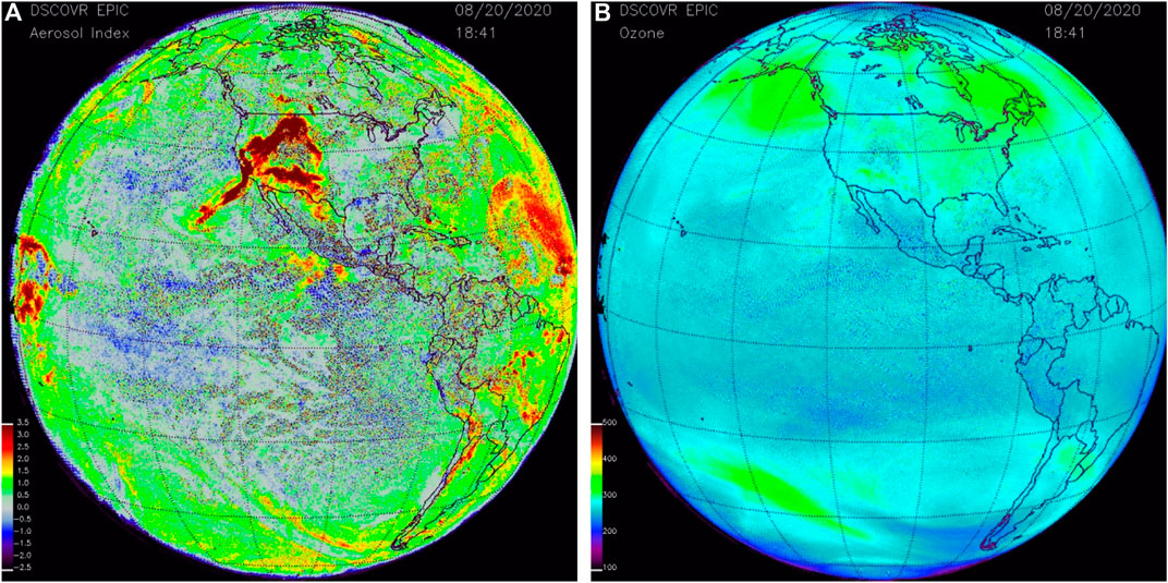
FIGURE 1. EPIC synoptic maps of the aerosol index (A) and TOZ (B) on August 8, 2020, at 18:41 UTC. Elevated levels of aerosols (AI>5) are clearly seen over western United States from massive wildfires. The ozone algorithm’s linear spectral dependence of reflectivity provides effective corrections for aerosol contamination. The corrected ozone fields are smooth without any apparent artificial structures imposed by wildfires. Ozone averaged over the aerosol contaminated area agrees well with the surrounding area.
The ozone version 3 retrieval algorithm accounts for ozone and temperature profile shape variations using seasonal zonally averaged climatology of ozone (McPeters and Labow, 2012) and temperature profiles. Calculated EPIC sun-normalized radiances stored in LUT are adjusted for differences between the seasonal climatological ozone (or temperature) profiles and the standard profiles.
Cloud height retrievals are obtained from EPIC oxygen A-band absorption measurements at 764 ± 0.2 nm and its reference wavelength 779.5 ± 0.3 nm (Yang et al., 2019). The EPIC simultaneous cloud-height product is now used in version 3 EPIC ozone algorithm for two purposes: 1) to adjust the scene surface pressure to properly simulate EPIC radiances; and 2) to estimate the unretrieved amount of ozone beneath clouds. The ozone climatology (McPeters and Labow, 2012) is used to substitute partial ozone columns below clouds, and the error in estimating cloud height for the high-altitude convective clouds can lead to errors in estimating total and tropospheric ozone columns in presence of such clouds. If the A-band cloud pressure height is not available (∼2–3% of EPIC images that are flagged in the L2 product), the ozone retrieval algorithm uses cloud effective pressure height from the OMI-based Optical Centroid Pressure (OCP) climatology (Vasilkov et al., 2008), used for all EPIC images in previous EPIC ozone versions. Figure 2 demonstrates how the simultaneous EPIC cloud height product helps reduce features in the synoptic TOZ maps produced by a large-scale convective cyclone. This is particularly important for tropospheric ozone studies that are sensitive to errors caused by the presence of clouds.
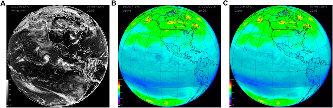
FIGURE 2. EPIC synoptic maps of reflectivity derived from 380 nm channel (A) and EPIC retrieved TOZ processed using OPT climatology (B) and simultaneous A-Band cloud height (C). The cyclonic activity in the tropical Pacific area west from Central America is clearly seen in the reflectivity map (A). The TOZ map derived with climatological cloud heights (B) has artificial structures that are co-located with the cyclones. When the simultaneous cloud height product from EPIC is used in the ozone algorithm (C) it reduces artificial structures in the derived synoptic TOZ maps.
To evaluate consistency of EPIC TOZ, we compared retrievals derived from two different triplets. The EPIC algorithm switches between 317.5 and 325 nm channels depending on optical depth conditions. At low optical depth (τ < 1.5), which corresponds to small and moderate SZA and SLA, the algorithm uses the 317.5 nm channel. When τ > 1.5, the algorithm switches to the 325 nm triplet that more easily penetrates to the surface. Since the natural ozone variability in the tropics is relatively low, we should expect very little changes in retrieved TOZ as a function of SZA or SLA. Therefore, we can evaluate consistency of EPIC retrievals as shown in Figure 3 by looking at the tropical zonal mean values retrieved from two triplets. The plots in Figure 3 show that TOZ averages derived with the 317 nm triplet (black lines) have very small variations at low and moderate SZA/SLA but starts to deviate when SZA/SLA > ∼70°. Larger errors in ozone retrievals at high SZA/SLA are related to the accuracy of radiance simulations using an approximation for atmospheric sphericity.
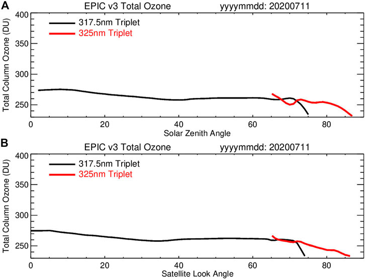
FIGURE 3. EPIC version-3 total column observations (in DU) on July 11, 2020 averaged for an entire day over a wide equatorial zone (20°S-20°N) as a function of SZA (A) and SLA (B). EPIC retrievals with 317.5 nm triplet are shown in black and 325 nm triplet in red. In this study, we use EPIC total ozone retrievals from 317.5 nm triplet only (algorithm flag equal 1, or 101, or 111) and limit SZA and SLA to less than 70°.
Figure 3 reveals inconsistency between EPIC 325 nm retrievals (red lines) and 317 nm retrievals (black lines) when they overlap. Since the 325 nm triplet has reduced ozone sensitivity compared to the 317 nm triplet, the retrieval errors in measured and simulated radiances will be amplified with the 325 nm triplet. These results are also supported by comparison with external measurements. Conditions with high optical depth typically correspond to early morning and late afternoon hours at the edges of the EPIC images, where EPIC has larger biases compared to other instruments (see Supplementary Figure S4). For scientific analysis, we recommend using EPIC total ozone retrievals from 317.5 nm triplet only (which corresponds to algorithm flag equal 1, or 101, or 111) and limiting the SZA and SLA to less than 70°. In this study EPIC data had been filtered using these criteria.
EPIC Tropospheric Ozone Algorithm
To derive tropospheric column ozone (TCO) from EPIC, an independent measure of the stratospheric ozone column is needed. The stratospheric column is then subtracted from EPIC TOZ to obtain tropospheric column ozone. Limb sounders like Aura MLS and OMPS LP have dense samplings and provide an accurate estimate of stratospheric ozone with high vertical resolution (e.g., Hubert et al., 2016; Kramarova et al., 2018; Wargan et al., 2020). These sounders are flown on polar-orbiting satellites and make measurements at the same local solar time with ∼14 orbits a day. Several techniques were tested to fill gaps between the orbits including the wind-trajectory method and data assimilation (Ziemke et al., 2014). Our analysis shows that the assimilated stratospheric ozone profiles provide the best overall measure of the stratospheric column ozone. We use the Modern-Era Retrospective analysis for Research and Applications, Version 2 (MERRA-2) ozone fields (Gelaro et al., 2017; Wargan et al., 2017) for this purpose. MERRA-2 assimilated stratosphere column ozone was found to agree within ±1–2 DU and standard deviations 2–4 DU with original MLS along-track measurements from the tropics to high latitudes. The MERRA-2 data assimilation system ingests Aura OMI v8.5 total ozone and MLS v4.2 stratospheric ozone profiles to produce global synoptic maps of ozone profiles from the surface to the top of the atmosphere; for our analyses we use MERRA-2 ozone profiles reported every 3 hours (0, 3, 6, … , 21 UTC) at a resolution of 0.625° longitude × 0.5° latitude (GMAO, 2015). MERRA-2 ozone profiles were integrated vertically from the top of the atmosphere down to tropopause pressure to derive maps of stratospheric column ozone. Tropopause pressure was determined from MERRA-2 re-analyses using standard PV-θ definition (2.5 PVU and 380 K). The resulting maps of stratospheric column ozone at 3-h intervals from MERRA-2 were then space-time collocated with EPIC footprints and subtracted from the EPIC total ozone, thus producing daily global maps of residual tropospheric column ozone sampled at the precise EPIC pixel times. These measurements of tropospheric ozone were further binned to 1o latitude × 1o longitude resolution. Figure 4 shows a schematic diagram that demonstrates the residual approach.
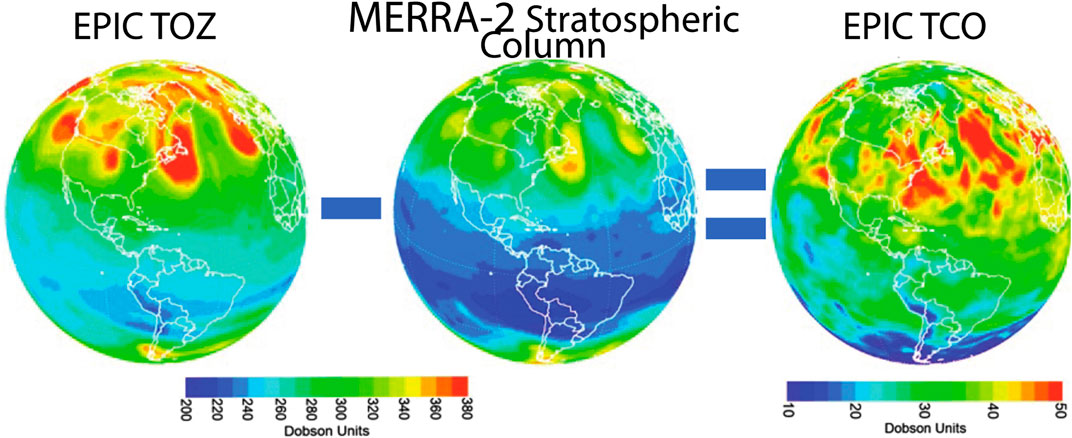
FIGURE 4. Schematic illustration of the residuals approach for deriving tropospheric ozone columns. The left plot shows a synoptic TOZ map derived from EPIC on June 24, 2019. The center plot shows a map of stratospheric ozone column from MERRA-2 for the same time. The TCO is derived by subtracting MERRA-2 stratospheric column from TOZ.
UV measurements have reduced sensitivity to ozone changes in the boundary layer. To facilitate error analysis, Column Weighting Functions (CWF) have been included in EPIC version 3 processing (see in the Supplementary Material) to help users interpret EPIC total ozone retrievals and indicate the weight of measurements in each layer. The shape of CWF are determined by the sensitivity of measured albedos to changes in ozone in different atmospheric layers. CWF are typically close to 1 in all layers except for the boundary layer (Supplementary Figure S1) indicating that the measurements are very sensitive to ozone changes in those layers. CWF in the lowest boundary layer ranges between 0 and 0.7, with low values close to 0 observed over high terrain or high clouds when measurements in the boundary layer are not available. CWF represent the fraction of ozone variations in that layer that can be retrieved. The magnitude of CWF in the boundary layer depends on SZA/SLA, reflectivity, and scene pressure (terrain height).
For comparisons with independent measurements like sondes, we need to account for the limited sensitivity of UV satellite measurements to the variability of ozone in the low troposphere including the boundary layer (BL) below ∼700 hPa. To do this, we used simulated tropospheric ozone derived from GEOS-Replay (Strode et al., 2020) constrained by the MERRA-2 meteorology through so-called replay method, whereby the analysis increments recalculated from MERRA-2 are used by the GEOS model in dynamical tendency calculations (Orbe et al., 2017). This correction represents a seasonal-cycle adjustment, since ozone variability in the troposphere including BL is largely due to the seasonal-cycle. From the GEOS-Replay simulation we constructed a 12-years (2005–2016) average global seasonal climatology of tropospheric ozone columns in the BL based on 365 days of the year at 1o × 1o horizontal gridding. To estimate adjustments to EPIC TCO, we first calculate the differences in BL ozone between this seasonal model-based climatology and the zonal-mean apriori values used in the EPIC retrieval algorithm (the ML climatology from McPeters and Labow, 2012). We then applied EPIC measured CWF to these BL ozone differences to estimate the ozone amount that EPIC measurements miss due to reduced sensitivity in the bottom layer (layer 0: 506 hPa -1,013 hPa). These corrections are then added to the EPIC tropospheric ozone columns to account for ozone variability in the BL (see in the Supplementary Material). Our analysis indicates that the global patterns for the corrections are very persistent between years dominated by strong seasonal variability.
Figure 5 shows the spatial distribution of the BL corrections for October 20, 2020, based on the GEOS-Replay model. There is a clear wave-1 structure in these corrections with a negative error of ∼ 2–6 DU over the tropical Pacific Ocean. This is because the ML apriori monthly zonal means do not capture longitudinal ozone variability. Negative corrections also correspond to places with high terrain. Positive corrections such as those over Africa, the Arabian Peninsula, India, and east China are regions of seasonally recurring biomass burning and other pollution that cause an increase in the BL ozone.
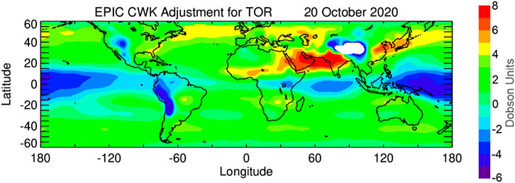
FIGURE 5. Spatial map of the CWF adjustment for the EPIC TCO due to reduced EPIC sensitivity to BL ozone for 20 October 2021. This correction is derived by applying EPIC CWFs for the bottom layer (506 hPa-1000 hPa) to the differences between GEOS-Replay model and ML apriori ozone.
Tropospheric ozone derived from satellite instruments prior to EPIC has been limited to maps sampled at fixed local times. A great advantage of EPIC is that tropospheric maps can be made every 1–2 h from the sunlit portion of the Earth with samples across the range of local solar times. Such maps provide information at times not sampled by polar orbiting satellites, allowing us to better capture and study short-scale, regional variability of tropospheric ozone.
Correlative Satellite Measurements
To validate EPIC ozone measurements, we use data obtained from two satellite sensors that operate on board polar orbiting satellites, OMI (Ozone Monitoring Instrument) and OMPS (Ozone Mapping and Profiling Suite). OMPS was launched in October 2011 on the Suomi National Polar-orbiting Partnership (SNPP) satellite and includes both nadir- and limb-viewing modules. In this study we will use total ozone maps derived from OMPS Nadir Mapper (NM). The NM is a hyperspectral imaging push-broom sensor with a 110° cross-track field of view (FOV), 35 cross-track bins, and a 0.27° along track slit width corresponding to a 50 × 50 km2 resolution. It measures solar backscattered ultraviolet radiation in a spectral range from 300 to 380 nm. The OMPS NM algorithm is based on the NASA version 8 total ozone algorithm (Bhartia and Wellemeyer, 2002) and uses a pair of wavelengths to derive total ozone. The ozone absorption cross-sections used in the OMPS NM algorithm are the same ones used for EPIC (Daumont et al., 1992; Malicet et al., 1995; Brion et al., 1998). The most recent version 2.1 of OMPS NM, which we used in this study, has been evaluated by (McPeters et al., 2019). They found that total column ozone data from the OMPS NM agree well with NOAA-19 SBUV/2 with a zonal average bias of −0.2% over the 60∘ S to 60∘ N latitude zone.
OMI, onboard the Aura satellite, started taking regular measurements in August 2004. OMI employs a hyperspectral imaging CCD in a push-broom mode to observe solar backscatter radiation in the 270–500 nm spectral range. The OMI sensor provides 60 cross-track bins with a FOV at nadir of about 13 km × 25 km. The wide scanning swath and 90-min polar orbit of OMI provides daily global maps of total ozone at 13:30 local solar equator crossing time. In this study, we use version 8.5 of OMI ozone data, processed with the version 8 algorithm (Bhartia and Wellemeyer, 2002). The most significant enhancement in OMI v8.5 is that the longer wavelengths measured by OMI are used to infer cloud height on a scene-by-scene basis (Vasilkov et al., 2008). OMI data are processed using Bass and Paur (1984) ozone absorption cross-sections. In 2008 the OMI started to experience blockage of the center-right part of each swath caused by peeling of the protective film on the spacecraft. The affected cross-track positions are flagged and are not used in our analysis. Comparison of OMI total ozone retrievals with an ensemble of Brewer and Dobson instruments and satellite SBUV measurements shows 1–1.5% bias, and a small relative drift against SBUV of about 0.5% over 10 years (McPeters et al., 2015).
Correlative Ground-Based Measurements
We used a network of Brewer spectrophotometers at multiple locations to evaluate EPIC TOZ measurements. The Brewer instrument acquires measurements at five UV wavelengths (306.3, 310.1, 313.5, 316.8 and 320.0 nm) to retrieve total column ozone (Kerr et al., 1985). The Brewer spectrometers are routinely calibrated with a reference triad of Brewers located in Toronto (Fioletev et al., 2005). The daily Brewer total ozone values are reported to the World Ozone and Ultraviolet Data Center (WOUDC). Brewer spectrometers perform measurements throughout the day, but there are only a small number of stations that report hourly Brewer data with the rest reporting daily average ozone amounts. We used Brewer daily averages in this study.
Ozonesonde measurements launched on air balloons provide in-situ measurements of ozone vertical profiles in the troposphere and low stratosphere that provide valuable validation for EPIC TCO. In this study we use measurements from 12 stations with several stations updated into year 2020. There is about one measurement per week at many sonde locations. We use daily measurements from Southern Hemisphere ADditional OZonesondes (SHADOZ) (Thompson et al., 2017; Witte et al., 2017), World Ozone and Ultraviolet Data Center (WOUDC) and Network for the Detection of Atmospheric Composition Change (NDACC). In our analysis, each ozone profile was integrated vertically from ground up to the tropopause to derive TCO. Tropopause height was determined the same as for EPIC TCO using MERRA-2 analyses with standard PV-θ definition (2.5 PVU, 380 K).
The ground-based Pandonia Global Network (PGN) uses temperature stabilized Avantes spectrometers in each Pandora instrument that simultaneously acquires direct-sun measurements in 300–525 nm range in oversampled steps of 0.5 nm every 40 s. Stray light from longer wavelengths is suppressed by using a short-wavelength bandpass filter. The Pandora ozone retrieval algorithm is based on an optimized spectral fitting within the ozone absorption range after correcting for aerosol amounts (Tzortziou et al., 2012; Herman et al., 2015; Herman et al., 2017). There are over 50 operating Pandora instruments within PGN and a number of additional Pandoras at various location through the world that are not yet incorporated into the official PGN.
Results
Evaluation of EPIC TOZ
To evaluate the accuracy of EPIC calibrations, we compared EPIC version 3 TOZ retrievals with correlative satellite observations from OMPS NM and OMI. Figure 6 shows mean differences in Dobson Units (DU) between EPIC version 3 and OMPS and OMI as a function of latitude for different seasons (color lines). The mean differences were calculated over a period from the beginning of the EPIC mission in June 2015 up to the end of 2020. The EPIC data have been filtered as described above in EPIC Total Ozone. The data in Figure 6 were first averaged monthly and zonally prior to calculating these 6-years differences. The mean biases are mostly within ±5–7 DU (or 1.5–2.5%). The biases between EPIC and OMI and EPIC and OMPS are smaller and mostly positive in the tropical region (30°S-30°N). Outside the tropics, biases are larger and vary seasonally. In the SH biases are mostly negative with stronger biases during SH summer in January (Figure 6, black lines). The biases are somewhat smaller between EPIC and OMI particularly in the tropics and NH (Figure 6B), while differences with OMPS in the NH tend to be larger and negative in April and October (Figure 6A). During NH summer in July the biases between EPIC and OMPS rapidly change at higher latitudes turning from positive to negative. Differences between Figures 6A,B indicate the magnitude of differences between OMI and OMPS TOZ.
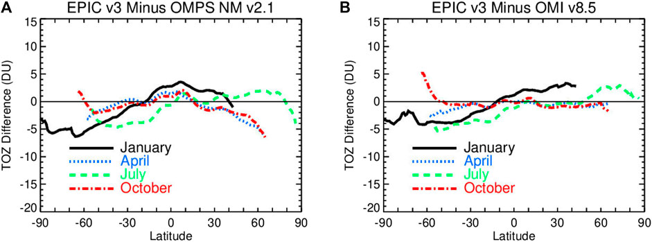
FIGURE 6. Mean biases in TOZ between EPIC v3 and OMPS NM v2.1 (A) and EPIC v3 and OMI v8.5 (B) in DU. Biases are shown for 4 months (shown in different colors) and calculated over period from June 2015 to December 2020. Only EPIC retrievals with the algorithm flag equal to 1, or 101, or 111 and SZA and SLA <70° were used in these comparisons.
To evaluate the effect of the EPIC cloud correction implemented in version 3 by utilizing simultaneous cloud height retrievals from the EPIC oxygen A-band channel, we compared EPIC and OMI TOZ retrievals for different conditions: all coincident cases with reflectivity 0 < R < 1, low-reflectivity cases R < 0.15, and cases with large reflectivity R > 0.7 (see Figure 7). The cloud height correction in the OMI algorithm uses the Optical Centroid Pressure (OCP) approach (Vasilkov et al., 2008) that utilizes OMI measurements in visible range between 460–490 nm. This algorithm is completely independent from the EPIC A-Band cloud heigh retrievals (Yang et al., 2019). There is a very good agreement between the two methods with differences less than 50 hPa over a broad range of cloud fraction values (see Supplementary Figure S2), which would result in an offset of less than 1 DU. The offset between two cloud height algorithms is larger at very low cloud fraction (<0.1), but it has almost no effect on retrieved ozone.
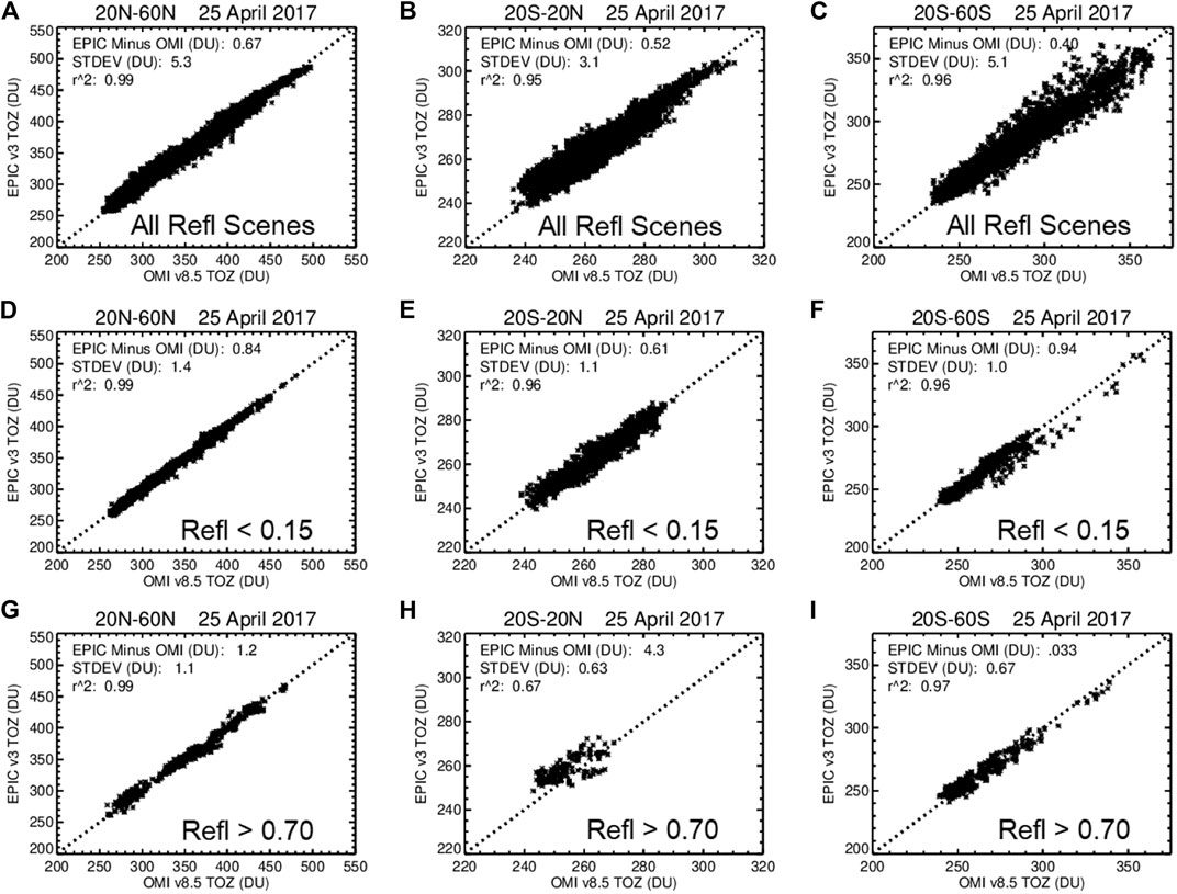
FIGURE 7. Comparisons between coincident EPIC and OMI TOZ measurements on April 25, 2017 in Dobson Units for all conditions (A–C), for cases with low scene reflectivity R < 0.15 with small cloud fraction and low-altitude clouds (D–F), and for cases with reflectivity values above >0.7 (G–I) that effectively corresponds to conditions with high-altitude convective clouds. The comparisons are binned in 3 wide latitude zones: 20°N-60°N (left column), 20°S-20°N (center column) and 20°S-60°S (right column). The mean differences and standard deviations are shown on each panel.
Our analysis has revealed that the mean biases between EPIC and OMI TOZ remain the same for two subsets (R < 0.15 and 0 < R < 1, see Figures 7A–F). That means the cloud correction implemented in version 3 does not produce systematic errors in the EPIC TOZ retrievals. There is an increase in standard deviations of differences for the subset where all conditions (0 < R < 1) were included (Figures 7A–C). This is consistent with our expectations that the cloud correction would produce random noise in the retrieved ozone fields but not a systematic bias. When the scene reflectivity exceeds 0.7 it typically corresponds to conditions with large cloud fraction and high-altitude, convective clouds. The biases increase in the tropics between the two instruments for R > 0.7, but there is no change in mid-latitudes. A fraction of these increased biases in the tropics might be due to consistently larger cloud heights derived from the A-Band for high cloud fractions (see Supplementary Figure S2). Additionally, differences in cloud coverage at the time of satellite measurements and satellites FOVs can contribute as well.
We also examined the relative degree of agreement between EPIC TOZ and ground-based measurements obtained from Brewer and Pandora instruments. The list of Brewer, Pandora and sonde stations used in this study is provided in Supplementary Table S1. Figure 8 shows time series of daily mean Brewer and EPIC TOZ measurements at six locations in 2018. These stations represent a wide range of latitudes with a long available record of daily Brewer measurements in 2015–2020. We did not include stations at high latitudes to avoid EPIC measurements at SZA and SLA that exceed 70°. These plots show sub-seasonal changes in TOZ as measured by EPIC and Brewers. The observed biases with Brewer measurements are within the range of differences found with satellite observations. There is a consistently high correlation between EPIC and Brewer measurements (r2 > 0.96), indicating that EPIC can accurately capture day-to-day variations in TOZ.
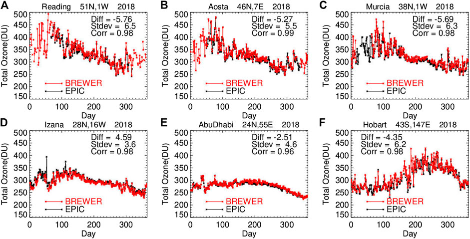
FIGURE 8. Time series of daily-average Brewer TOZ measurements (red) and EPIC v3 daily overpasses (black) at 6 ground-based stations world-wide in 2018: (A) Reading, United Kingdom, (B) Aosta, Italy, (C) Murcia, Spain, (D) Izana, Spain, (E) Abu Dhabi, United Arab Emirates, and (F) Hobard, Australia. The mean differences, standard errors of the mean in DU and correlation coefficients are shown at each panel.
Figure 9 shows comparisons between EPIC and Pandora TOZ from 4 selected sites in the NH and SH where there is a long record of ground-based data from well-calibrated Pandora spectrometer instruments. We also compared with overpasses derived from OMI and OMPS NM. EPIC TOZ overpasses for each selected site include about 3–4 samples per day separated by 1–2 h, while OMI and OMPS overpasses have only 1 to 2 points per day, with most samples consisting of 1 point per day. When there are two points from consecutive polar orbits, they are separated by about 90 min. The ground-based Pandora data consists of ozone samples obtained every 40 s throughout each day for solar zenith angles SZA less than 70°. The time span of PGN Pandora data is much less than that for satellite data. Because of the different fields of view FOV (EPIC 20 × 20 km2, OMI 13 × 24 km2, OMPS 50 × 50 km2 and Pandora about 50 × 50 m2) and different sampling times (UT), the comparisons in Figure 9 are done for 3-months averages to verify calibration and retrieval algorithm rather than individual scene comparisons. The noise level in comparisons drop significantly depending on the averaging period (see Supplementary Figure S5). The 3-months averages (solid lines in Figure 9) match closely for all four instruments. The mean differences between EPIC and OMI and OMPS are smaller than 1% at all stations and consistent with zonally averaged results shown in Figure 6. Pandora TOZ measurements in the current version (PGN version 0P1) have significant differences with all three satellite instruments, but closely track the observed TOZ variation.
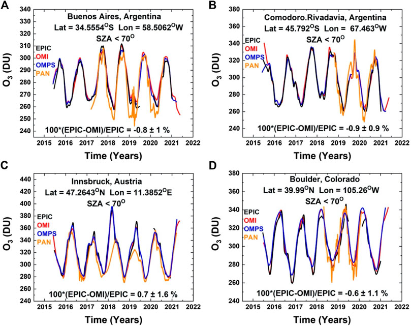
FIGURE 9. A comparison of EPIC TOZ time series (black) with Pandora (red), OMI (blue) and OMPS (orange) at four ground-based stations: Buenos Aires, Argentina (A), Comodoro, Argentina (B), Innsbruck, Austria (C), and Boulder, Colorado United States (D). The lines are a Local-Linear Least-Squares (LOESS) fit to the data (Cleveland, 1979) equivalent to approximately a 3-months running average. The biases between EPIC and OMI (in %), indicated in each panel, are done for 3-months averages. EPIC data had been screened as described in Earth Polychromatic Imaging Camera Total Ozone.
To evaluate EPIC performance at short time scales, we have compared EPIC with ground-based Pandora and coincident OMI measurements at two ground-based locations over 1-year period (Figure 10). There is a lot of variability in TOZ during winter and spring at the mid-latitude station in Greenbelt, Maryland (Figure 10A), showing that EPIC agrees well with both Pandora and OMI. TOZ is lower in summer and autumn months as a part of the TOZ seasonal cycle. Pandora in Greenbelt seems to underestimate TOZ in summer months compared to both OMI and EPIC. Measurements at Fairbanks, Alaska show a significant seasonal change where TOZ is close to 400–450 DU in winter and then gradually dropping to ∼250 DU in the late summer - early autumn (Figure 10B). EPIC captures these seasonal as well as smaller scale changes in TOZ compared to both Pandora and OMI. However, at high SZA (>70°) EPIC tends to underestimate TOZ compared to OMI. The two instruments also see ozone variability differently at high SZA conditions: OMI measurements are showing more small-scale variations (blue line in Figure 10B), while the EPIC curve (black line in Figure 10B) is smoother. This is partly because we considered all EPIC measurements at Fairbanks, including those from 325 nm triplet to cover winter months. These results suggest that retrievals from the 325 nm triplet, used at high SZA, are not just biased, but might also have less sensitivity to real changes in ozone. Further investigations are needed to understand the reason for reduced quality of 325 nm EPIC retrievals. Pandora measurements in Alaska also show low biases in summer months compared to EPIC and OMI.
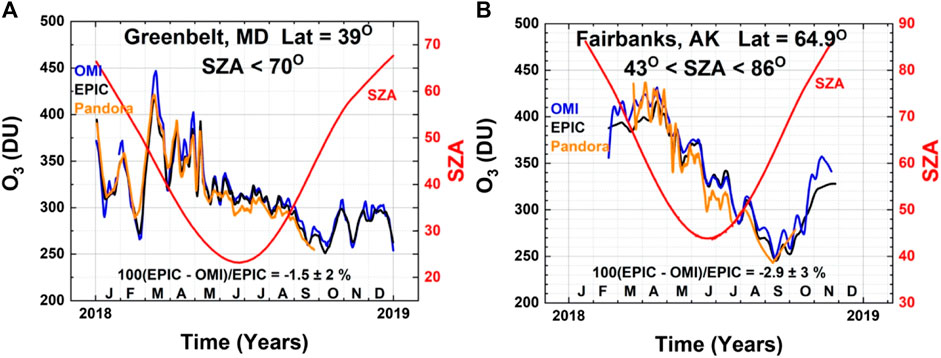
FIGURE 10. Comparisons of EPIC TOZ (in DU) with ground-based Pandora and satellite OMI TOZ measurements in 2018 at two locations: (A) Greenbelt, MD, United States and (B) Fairbanks, Alaska, United States. Plots show time series of TOZ measurements derived by fitting the LOESS (equivalent to a 3-weeks moving average) to all available EPIC (black lines), Pandora (orange) and OMI (blue) measurements at both locations. The red curve shows the average SZA for all EPIC measurements with a scale shown on the right hand. At Greenbelt only EPIC measurements with SZA <70° were used, while at Fairbanks all available EPIC measurements were included.
Evaluation of EPIC Tropospheric Column Ozone
To evaluate EPIC TCO we use sonde observations at multiple stations (Figure 11). For the comparisons with sondes, we applied corrections for the boundary layer ozone as described in Earth Polychromatic Imaging Camera Tropospheric Ozone Algorithm. In Figure 11 we also applied −3 DU constant adjustment to EPIC TCO everywhere. This constant adjustment decreases biases between EPIC and sonde TCO at all stations. The 3 DU bias can be a result of ∼0.3% error in 317.5 nm absolute radiance calibrations of EPIC, which is substantially below the ±1% quoted accuracy of EPIC and OMPS calibrations. Tropospheric ozone changes significantly with latitude and season. EPIC TCO accurately captures these variations from one station to another with the mean biases against independent sonde measurements of ±2.5 DU (or ∼10%). It is important to note that there are numerous sources of errors in the residual method used to derive EPIC TCO including uncertainties in stratospheric ozone column, tropopause height, cloud height. In addition, ozone sondes provide local measurements over the station, while satellite EPIC TCO represent gridded averages. Therefore, larger noise levels (captured by standard deviations of differences) in these comparisons are expected.
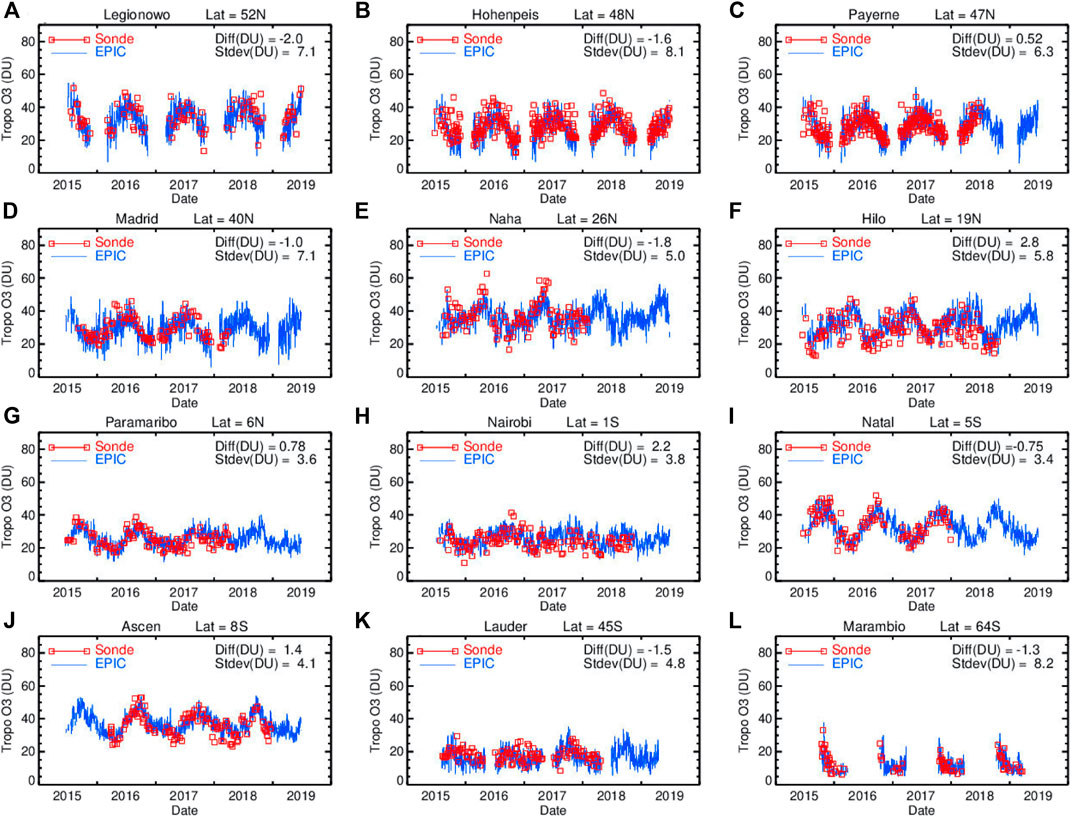
FIGURE 11. Time series of EPIC (blue lines) and sonde (red squares) daily TCO in 2015–2019 at 12 ground-based locations: (A) Leginowo, Poland; (B) Hohenpeissenberg, Germany; (C) Payerne, Switzerland; (D) Madrid, Spain; (E) Naha, Japan; (F) Hilo, United States; (G) Paramaribo, Suriname; (H) Nairobi, Kenya; (I) Natal, Brazil; (J) Ascension Island; (K) Lauder, New Zeland; (L) Marambio, Antarctica. Mean differences and standard deviations in DU between EPIC and coincident sonde TCO measurements are quoted in each panel.
Figure 12 shows the monthly zonal mean EPIC TCO as a function of time and latitude. It shows that on average TCO values in the SH are smaller than those in the NH, in agreement with our understanding of tropospheric ozone chemistry. The seasonal cycle is not very strong in the SH, while it is very pronounced in the tropics and NH. In the tropics, the seasonal cycle in TCO peaks in September-November due largely to lightning and biomass burning, with a minimum seen in January-March (e.g., Sauvage et al., 2007). In the NH, the seasonal peak varies from spring months in the tropics/subtropics to summer months in the mid-latitudes due to variations in combined spring-summer stratosphere-troposphere exchange (STE) and pollution (Lelieveld and Dentener, 2000; de Laat et al., 2005; Ziemke et al., 2006; and references therein).
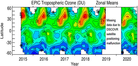
FIGURE 12. EPIC monthly zonal mean TCO as a function of time and latitude. These TCO values were adjusted with CWF to account for reduced sensitivity to the boundary layer. Results are shown with 3 DU steps.
EPIC did not make observations between late June 2019 and February 2020 due to malfunctioning of the satellite positioning (now corrected). After measurements resumed, there were no significant calibration changes. However, a substantial drop of ∼3–4 DU (∼5–10%) in TCO over much of the NH in spring and summer of 2020 can be seen in Figure 12. A part of these TCO reductions in 2020 appears to be related to the unprecedented strong, cold, and long-lasting stratospheric polar vortex over the Arctic in winter and spring 2019–2020 (Lawrence et al., 2020; Manney et al., 2020) that led to substantial polar ozone losses (e.g., DeLand et al., 2020). Ground-based ozone observations (Steinbrecht et al., 2021) confirmed a reduction in both total and tropospheric ozone in spring and summer 2020 attributing ∼25% of the reduction to the 2019/2020 Arctic ozone depletion. Another factor that potentially contributed to the observed reduction in EPIC TCO in the NH is related to the global COVID-19 pandemic. COVID-related measures in spring and summer 2020 resulted in the reduction of anthropogenic emissions including Volatile Organic Compounds (VOCs) and NOX (NO + NO2) which are precursors for tropospheric ozone production (e.g., Liu et al., 2020). Steinbrecht et al. (2021) found from ozonesonde analyses about 7% reduction in tropospheric ozone throughout the NH free troposphere in spring-summer 2020. The 2–4 DU (5–10%) reductions in zonal-mean EPIC TCO in the NH (Figure 12) are consistent with the 7% reductions described by Steinbrecht et al. (2021).
We also compared EPIC daily TCO with daily TCO derived from OMI and OMPS nadir-mapper satellite instruments. For OMI and OMPS (similar to EPIC), MERRA-2 stratospheric columns were space-time collocated with total ozone pixel measurements to derive TCO. Figures 13A–C show maps of TCO on July 7, 2020, as observed by these three satellite instruments. We note that EPIC TCO measurements in Figure 13, as with all EPIC TCO measurements presented in this study, include the CWF correction for the boundary layer ozone discussed in Earth Polychromatic Imaging Camera Tropospheric Ozone Algorithm, while OMPS and OMI TCO have not been corrected. There is a good agreement in spatial patterns of TCO such as increased tropospheric ozone over the Midwest and eastern coast of the United States that extends over the Atlantic Ocean due to extra-tropical weather variability. There are missing data in OMI measurements caused by the sensor’s row anomalies (i.e., seen as black bands in Figure 13B for OMI), but similarities in global patterns are seen. Figures 13D–I show one-to-one comparisons between EPIC TCO with OMI and OMPS TCO for three latitude zones (indicated). There is a good agreement in the NH and tropics with mean biases of less than ±2 DU, but there are strong negative biases of −4 to −5 DU in the SH with increased standard deviations. Similar negative biases were also observed in EPIC TOZ in the SH extra-tropics with respect to OMI and OMPS (see Figure 6) with the largest biases in July and January of about −5 DU.
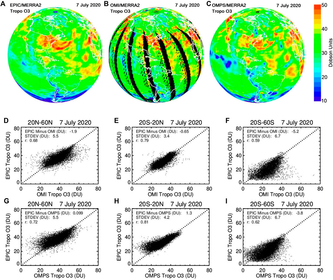
FIGURE 13. The three upper color panels show daily maps of TCO (in DU) derived from EPIC (A), OMI (B) and OMPS (C) on July 7, 2020. The lower panels (D–I) show scatter plots of EPIC TCO against coincident OMI (center row, D–F) and OMPS (lower row, (G–I)). The scatter plots are shown for three wide latitude zones: 20°N-60°N (left column, D,G), 20°S-20°N (center column, E,H) and 20°S-60°S (right column, F,I). The mean differences and corresponding standard deviations (both in DU) are shown in each panel along with correlation coefficients.
We compared coincident EPIC daily TCO with OMI and OMPS daily TCO over the entire EPIC operational period between June 2015 and December 2020 and calculated offsets and standard deviations as a function of month and latitude (Figure 14). We found that in the NH the biases are mostly positive and ranging between 1 and 3 DU. The biases with respect to OMPS become negative and increase at high northern latitudes. In the SH, EPIC TCO tends to have negative biases with OMI and OMPS, particularly in winter and summer months. A similar pattern can be seen in Figure 6 between EPIC and OMPS TOZ. The comparisons are less noisy in the tropics and during mid-latitude summer in the NH with standard deviations of 3–5 DU (10–15%). In wintertime in the NH the noise tends to increase almost by a factor of two up to 9 DU (or 40–50%), even though the seasonal peak in TCO occurs during the summer. These indicate that the main uncertainties in the tropospheric ozone detection are related to increased errors in deriving TOZ at high SZA and reduced accuracy of stratospheric ozone columns in wintertime. Stratospheric ozone variability is increasingly larger in the winter hemisphere (e.g., Kramarova et al., 2018) as well as variations in tropopause heights, which would result in increased uncertainties in estimating stratospheric ozone columns from MERRA-2.
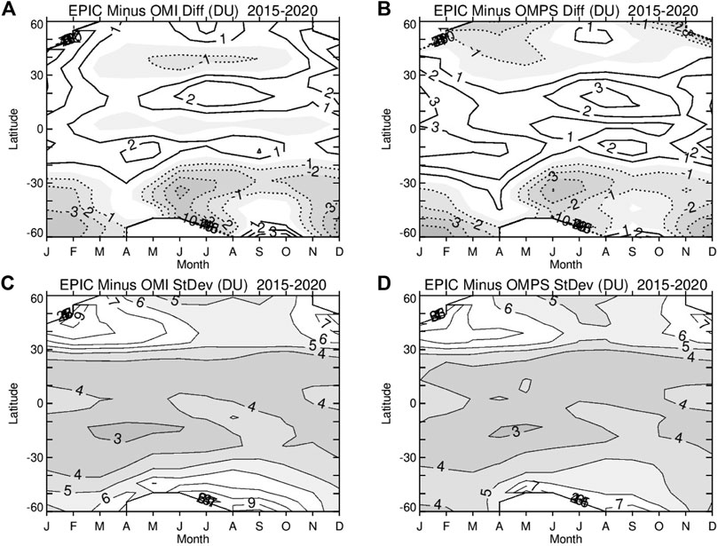
FIGURE 14. Differences (in DU) between coincident EPIC TCO daily values and those from (A) OMI and (B) OMPS over the period between June 2015 and December 2020 shown as function of month and latitude. The positive differences are shown as solid lines in a-b, and negative as dashed lines and shaded. The corresponding 1-sigma standard deviations of the differences with OMI and OMPS are plotted as (C–D), respectively.
Summary and Discussion
In this study we evaluated EPIC ozone products processed with the version-3 ozone algorithm, which includes several modifications compared to previous version 2 (Herman et al., 2018). First, an improved geolocation of EPIC scenes is applied in Version 3 Level 1 product (Blank et al., 2021) that ensures the filters are viewing the same geographic scene and solar/view angles are accurately estimated for each EPIC pixel thereby reducing errors in ozone retrievals. Second, the inclusion of simultaneous cloud-height information from EPIC A-Band (Yang et al., 2019) improves the scene pressure and the estimated ozone amount below the cloud. We have demonstrated in this study that the cloud correction based on the simultaneous EPIC A-Band retrievals reduces features in the EPIC total ozone fields imposed by cyclonic activity and does not produce systematic biases in ozone. The third change is the addition of corrections for ozone and temperature profile shapes in the retrieval algorithm. And finally, version 3 includes column weighting functions and algorithm/error flags for each observation to facilitate error analysis.
Comparisons of EPIC total ozone columns with satellite instruments (SNPP OMPS and Aura OMI) demonstrated good agreement with mean biases within ±5–7 DU (or 1.5–2.5%). Outside of the tropics, biases with other satellite instruments show seasonal variability. In the SH, EPIC shows mostly negative biases compared to both OMI and OMPS with stronger biases during SH summer in January. Comparisons of daily EPIC total ozone columns with ground-based Brewer instruments at 6 sites show good agreement between EPIC and Brewers in capturing day-to-day variations in total ozone with consistently high correlation (r2 > 0.9). The mean differences between EPIC and Brewers are within the same range as with satellite observations, and there are no obvious latitudinal patterns.
We examined EPIC tropospheric ozone columns derived by subtracting MERRA-2 stratospheric ozone columns from EPIC total ozone measurements and adjusted for reduced EPIC sensitivity to the boundary layer ozone. We compared daily TCO with matching TCO derived from ozonesondes at 12 stations over the period 2015–2019. We found that after removing a constant 3 DU offset between EPIC and sondes globally (at all stations) the biases in tropospheric column ozone are within ±2.5 DU (or ∼±10%). We found that EPIC TCO captures latitudinal and seasonal variations in tropospheric ozone. The 3 DU offset can be a result of ∼0.3% error in 317.5 nm absolute radiance calibrations of EPIC (note, that it is substantially lower than the quoted accuracy, ±1%, of EPIC and OMPS calibrations). In addition, we compared coincident EPIC daily TCO with OMI and OMPS daily TCO over the entire EPIC operational period between June 2015 and December 2020 and found that biases in tropospheric column ozone have similar magnitude and patterns to those seen in total ozone comparisons.
Analysis of time series of zonal mean EPIC TCO indicated a substantial drop of ∼2–4 DU (∼5–10%) over much of the NH in spring and summer of 2020, which is consistent with the 7% reductions in tropospheric ozone from ground-based observations described by Steinbrecht et al. (2021). A part of this reduction is related to unprecedented Arctic stratospheric ozone losses in winter-spring 2019/2020 and to reductions in ozone precursor pollutants due to the COVID-19 pandemic.
In this study, we mostly used EPIC data derived from the 317 nm triplet and limited SZA and SLA to less than 70°. Our analysis revealed consistent biases between EPIC retrievals derived from the two triplets (317 and the 325 nm) that cannot be explained by the natural ozone variability. We demonstrated that the inclusion of the 325 nm EPIC retrievals led to substantial increase in systematic biases. The EPIC ozone algorithm switches to 325 nm triplet for conditions with high optical depth, which typically correspond to high SZA and SLA. The exact reasons for increased errors in EPIC ozone retrievals derived from the 325 nm triplet are under investigation. Errors in radiance simulations with a pseudo-correction for atmospheric sphericity at high SZAs and SLAs, reduced sensitivity to ozone at 325 nm compared to 317 nm, and uncertainties in absolute calibrations of the two EPIC channels are the main factors to consider. The current exclusion of EPIC 325 nm retrievals limits applications of EPIC data for studying ozone variability in early morning and late afternoon hours or at polar latitudes in months with high SZAs.
Data Availability Statement
Publicly available datasets were analyzed in this study. This data can be found here: EPIC Total ozone data are available at https://eosweb.larc.nasa.gov/project/DSCOVR/DSCOVR_EPIC_L2_TO3_03 EPIC overpass data for TOZ and TCO, used in this paper, are available at https://avdc.gsfc.nasa.gov/pub/DSCOVR/Kramarova_et_al_Data/. SNPP OMPS NM v2.1 and Aura OMI v8.5 total ozone data can be downloaded from https://ozoneaq.gsfc.nasa.gov/data/ozone/. OMPS and OMI overpass over ground-based stations are available at https://acd-ext.gsfc.nasa.gov/anonftp/toms/. Ground-based Brewer measurements can be found at WOUDC (https://woudc.org/), NDACC (http://www.ndsc.ncep.noaa.gov/). Pandora total ozone measurements are available at http://data.pandonia-global-network.org/. Sondes: SHADOZ (https://tropo.gsfc.nasa.gov/shadoz/), WOUDC (https://woudc.org/), NDACC (http://www.ndsc.ncep.noaa.gov/). MERRA-2 data can be found here: https://disc.gsfc.nasa.gov/datasets?project=MERRA-2.
Author Contributions
NK is the leading author of the paper. She was responsible for writing the paper, analyzing results, drawing conclusions, and interacting with co-authors. JZ is responsible for tropospheric ozone algorithm. For this paper, JZ compared EPIC TOZ and TCO with measurements from OMI/OMPS, Brewers and ozonesondes. L-KH is responsible for maintaining and developing of the EPIC ozone retrieval algorithm. For this paper, L-KH evaluated effects of various algorithmic parameters (like cloud heights, aerosol correction, Level 1 adjustments) on changes in retrieved ozone. JH was responsible for comparisons between EPIC and Pandora measurements, as well as for evaluation of EPIC and OMI/OMPS total ozone overpasses at several ground-based stations. KW contributed to this paper by helping with MERRA-2 stratospheric ozone profiles needed for EPIC tropospheric ozone derivation. CS helped with the development of the EPIC ozone retrieval algorithm and with calibration of EPIC UV channels by providing calibrated OMPS measurements. GL helped with comparisons of EPIC TOZ with Brewer measurements. LO assisted with interpretation and application of the GEOS-Replay model data.
Funding
NK, JZ and L-KH were supported by NASA ROSES proposal “Improving total and tropospheric ozone column products from EPIC on DSCOVR for studying regional scale ozone transport” (18-DSCOVR18-0,011, DSCOVR Science Team). JH is supported DSCOVR/EPIC NASA project under UMBC task 00,011,511. L-KH, KW, CS and GL were supported by SSAI Support for Atmospheres, Modeling, and Data Assimilation (NNG17HP01C) contract with NASA GSFC. Luke Oman was supported by NASA Modeling, Analysis, and Prediction (MAP) program.
Conflict of Interest
L-KH, KW, CS, and GL were employed by Science Systems and Applications, Inc. (SSAI).
The remaining authors declare that the research was conducted in the absence of any commercial or financial relationships that could be construed as a potential conflict of interest.
Publisher’s Note
All claims expressed in this article are solely those of the authors and do not necessarily represent those of their affiliated organizations, or those of the publisher, the editors and the reviewers. Any product that may be evaluated in this article, or claim that may be made by its manufacturer, is not guaranteed or endorsed by the publisher.
Acknowledgments
Authors would like to thank P.K. Bhartia (NASA GSFC) and David Haffner (SSAI/NASA GSFC) for constructive discussion of the results presented in this paper that helped to improve the manuscript. The GEOS-Replay simulation was supported by the NASA MAP program and the high-performance computing resources were provided by the NASA Center for Climate Simulation (NCCS). MERRA-2 is an official product of the Global Modeling and Assimilation Office at NASA GSFC, supported by NASA’s Modeling, Analysis and Prediction (MAP) program. Authors would like to thank the editor GS and three reviewers (YH, VN, and DF) for their thoughtful comments and suggestions that improved the manuscript.
Supplementary Material
The Supplementary Material for this article can be found online at: https://www.frontiersin.org/articles/10.3389/frsen.2021.734071/full#supplementary-material
References
Bass, A. M., and Paur, R. J. (1984). “The Ultraviolet Cross-Sections of Ozone. I. The Measurements,” in Proc. Quadrenniel Ozone Symp., Halkidiki, Greece, 3–7 September, 1984. Editors C. Zerefos, A. Ghazi, and Dordecht. Reidel, 606–616.
Bhartia, P. K., and Wellemeyer, C. W. (2002). “OMI TOMS-V8 Total O3 Algorithm,” in Algorithm Theoretical Baseline Document: OMI Ozone Products. Editor P. K. Bhartia, vol. II. ATBD-OMI-02, version 2.0, Aug. 2002.
Blank, K., Huang, L. K., Herman, J., and Marshak, A. (2021). EPIC Geolocation Front. Remote Sens.. (in preparation).
Brion, J., Chakir, A., Charbonnier, J., Daumont, D., Parisse, C., and Malicet, J. (1998). Absorption Spectra Measurements for the Ozone Molecule in the 350–830 Nm Region. J. Atmos. Chem. 30, 291–299. doi:10.1023/a:1006036924364
Caudill, T. R., Flittner, D. E., Herman, B. M., Torres, O., and McPeters, R. D. (1997). Evaluation of the Pseudo-spherical Approximation for Backscattered Ultraviolet Radiances and Ozone Retrieval. J. Geophys. Res. 102, 3881–3890. doi:10.1029/96jd03266
Cede, A., Huang, L.-K., McCauley, G., Herman, J., Blank, K., Kowalewski, M., et al. (2021). Raw EPIC Data Calibration. Front. Remote Sens. (in review). doi:10.3389/frsen.2021.702275
CEOS (2011). Report of the Committee on Earth Observation Satellites (CEOS) Atmospheric Composition Constellation (ACC) “A Geostationary Satellite Constellation for Observing Global Air Quality: An International Path Forward”. Available at: http://ceos.org/document_management/Virtual_Constellations/ACC/Documents/AC-VC_Geostationary-Cx-for-Global-AQ-final_Apr2011.pdf.
Cleveland, W. S. (1979). Robust Locally Weighted Regression and Smoothing Scatterplots. J. Am. Stat. Assoc. 74, 829–836. doi:10.1080/01621459.1979.10481038
Daumont, D., Brion, J., Charbonnier, J., and Malicet, J. (1992). Ozone UV Spectroscopy I: Absorption Cross-Sections at Room Temperature. J. Atmos. Chem. 15, 145–155. doi:10.1007/bf00053756
de Laat, A. T. J., Aben, I., and Roelofs, G. J. (2005). A Model Perspective on Total Tropospheric O3column Variability and Implications for Satellite Observations. J. Geophys. Res. 110, D13303. doi:10.1029/2004JD005264
DeLand, M. T., Bhartia, P. K., Kramarova, N., and Chen, Z. (2020). OMPS LP Observations of PSC Variability during the NH 2019–2020 Season. Geophys. Res. Lett. 47, e2020GL090216. doi:10.1029/2020gl090216
Dobber, M., Voors, R., Dirksen, R., Kleipool, Q., and Levelt, P. (2008). The High-Resolution Solar Reference Spectrum between 250 and 550 Nm and its Application to Measurements with the Ozone Monitoring Instrument. Sol. Phys. 249, 281–291. doi:10.1007/s11207-008-9187-7
Fioletov, V. E., Kerr, J. B., McElroy, C. T., Wardle, D. I., Savastiouk, V., and Grajnar, T. S. (2005). The Brewer Reference Triad. Geophys. Res. Lett. 32, L20805. doi:10.1029/2005GL024244
Gelaro, R., McCarty, W., Suárez, M. J., Todling, R., Molod, A., Takacs, L., et al. (2017). The Modern-Era Retrospective Analysis for Research and Applications, Version 2 (MERRA-2). J. Clim. 30, 5419–5454. doi:10.1175/JCLI-D-16-0758.1
Global Modeling and Assimilation Office (GMAO) (2015b). MERRA-2 inst3_3d_asm_Np: 3d,3-Hourly,Instantaneous,Pressure-Level,Assimilation,Assimilated Meteorological Fields V5.12.4, Greenbelt, MD, USA, Goddard Earth Sciences Data and Information Services Center (GES DISC). Accessed: [Data Access July 29, 2021]. doi:10.5067/QBZ6MG944HW0
Global Modeling and Assimilation Office (GMAO) (2015a). MERRA-2 inst3_3d_asm_Nv: 3d,3-Hourly,Instantaneous,Model-Level,Assimilation,Assimilated Meteorological Fields V5.12.4. Greenbelt, MD, USA: Goddard Earth Sciences Data and Information Services Center (GES DISC). Accessed: [Data Access Date]. doi:10.5067/WWQSXQ8IVFW8
Herman, J., Evans, R., Cede, A., Abuhassan, N., Petropavlovskikh, I., and McConville, G. (2015). Comparison of Ozone Retrievals from the Pandora Spectrometer System and Dobson Spectrophotometer in Boulder, Colorado. Atmos. Meas. Tech. 8, 3407–3418. doi:10.5194/amt-8-3407-2015
Herman, J., Evans, R., Cede, A., Abuhassan, N., Petropavlovskikh, I., McConville, G., et al. (2017). Ozone Comparison between Pandora #34, Dobson #061, OMI, and OMPS in Boulder, Colorado, for the Period December 2013-December 2016. Atmos. Meas. Tech. 10, 3539–3545. doi:10.5194/amt-10-3539-2017
Herman, J., Huang, L., McPeters, R., Ziemke, J., Cede, A., and Blank, K. (2018). Synoptic Ozone, Cloud Reflectivity, and Erythemal Irradiance from Sunrise to sunset for the Whole Earth as Viewed by the DSCOVR Spacecraft from the Earth-Sun Lagrange 1 Orbit. Atmos. Meas. Tech. 11, 177–194. doi:10.5194/amt-11-177-2018
Hubert, D., Lambert, J.-C., Verhoelst, T., Granville, J., Keppens, A., Baray, J.-L., et al. (2016). Ground-based Assessment of the Bias and Long-Term Stability of 14 Limb and Occultation Ozone Profile Data Records. Atmos. Meas. Tech. 9, 2497–2534. doi:10.5194/amt-9-2497-2016
Kerr, J. B., McElroy, C. T., Wardle, D. I., Olafson, R. A., and Evans, W. F. J. (1985). “The Automated Brewer Spectrophotometer,” in Atmospheric Ozone: Proceedings of the Quadrennial Ozone Symposium. Editors C. S. Zerefos, and A. Ghazi (Hingham, Mass: Springer), 396–401. doi:10.1007/978-94-009-5313-0_80
Kim, J., Jeong, U., Ahn, M.-H., Kim, J. H., Park, R. J., Lee, H., et al. (2020). New Era of Air Quality Monitoring from Space: Geostationary Environment Monitoring Spectrometer (GEMS). Bull. Am. Meteorol. Soc. 101 (1), E1–E22. Retrieved Jun 15, 2021, from https://journals.ametsoc.org/view/journals/bams/101/1/bams-d-18-0013.1.xml. doi:10.1175/bams-d-18-0013.1
Kramarova, N. A., Bhartia, P. K., Jaross, G., Moy, L., Xu, P., Chen, Z., et al. (2018). Validation of Ozone Profile Retrievals Derived from the OMPS LP Version 2.5 Algorithm against Correlative Satellite Measurements. Atmos. Meas. Tech. 11, 2837–2861. doi:10.5194/amt-11-2837-2018
Lawrence, Z. D., Perlwitz, J., Butler, A. H., Manney, G. L., Newman, P. A., Lee, S. H., et al. (2020). The Remarkably Strong Arctic Stratospheric Polar Vortex of Winter 2020: Links to Record‐Breaking Arctic Oscillation and Ozone Loss. J. Geophys. Res. Atmos. 125, e2020JD033271. doi:10.1029/2020JD033271
Lelieveld, J., and Dentener, F. J. (2000). What Controls Tropospheric Ozone?. J. Geophys. Res. 105, 3531–3551. doi:10.1029/1999JD901011
Liu, F., Page, A., Strode, S. A., Yoshida, Y., Choi, S., Zheng, B., et al. (2020). Abrupt Decline in Tropospheric Nitrogen Dioxide over China after the Outbreak of COVID-19. Sci. Adv. 6 (28), eabc2992. doi:10.1126/sciadv.abc2992
Malicet, J., Daumont, D., Charbonnier, J., Parisse, C., Chakir, A., and Brion, J. (1995). Ozone UV Spectroscopy. II. Absorption Cross-Sections and Temperature Dependence. J. Atmos. Chem. 21, 263–273. doi:10.1007/bf00696758
Manney, G. L., Livesey, N. J., Santee, M. L., Froidevaux, L., Lambert, A., Lawrence, Z. D., et al. (2020). Record‐Low Arctic Stratospheric Ozone in 2020: MLS Observations of Chemical Processes and Comparisons with Previous Extreme Winters. Geophys. Res. Lett. 47, e2020GL089063. doi:10.1029/2020GL089063
Marshak, A., Herman, J., Adam, S., Karin, B., Carn, S., Cede, A., et al. (2018). Earth Observations from DSCOVR EPIC Instrument. Bull. Amer. Meteorol. Soc. 99 (9), 1829–1850. doi:10.1175/BAMS-D-17-0223.1
McPeters, R. D., Frith, S., and Labow, G. J. (2015). OMI Total Column Ozone: Extending the Long-Term Data Record. Atmos. Meas. Tech. 8, 4845–4850. doi:10.5194/amt-8-4845-2015
McPeters, R. D., and Labow, G. J. (2012). Climatology 2011: an MLS and Sonde Derived Ozone Climatology for Satellite Retrieval Algorithms. J. Geophys. Res. 117, a–n. doi:10.1029/2011JD017006
McPeters, R., Frith, S., Kramarova, N., Ziemke, J., and Labow, G. (2019). Trend Quality Ozone from NPP OMPS: the Version 2 Processing. Atmos. Meas. Tech. 12, 977–985. doi:10.5194/amt-12-977-2019
Orbe, C., Oman, L., Strahan, S., Waugh, D., Pawson, S., Takacs, L., et al. (2017). Large-Scale Atmospheric Transport in GEOS Replay Simulations. J. Adv. Model. Earth Sy. 9, 2545–2560. doi:10.1002/2017MS001053
Sauvage, B., Martin, R. V., van Donkelaar, A., and Ziemke, J. R. (2007). Quantification of the Factors Controlling Tropical Tropospheric Ozone and the South Atlantic Maximum. J. Geophys. Res. 112 (D11), D11309. doi:10.29/2006JD008008
Seftor, C. J., Jaross, G., Kowitt, M., Haken, M., Li, J., and Flynn, L. E. (2014). Postlaunch Performance of the Suomi National Polar-Orbiting Partnership Ozone Mapping and Profiler Suite (OMPS) Nadir Sensors. J. Geophys. Res. Atmos. 119 (7), 4413–4428. doi:10.1002/2013JD020472
Stark, H. R., Moller, H. L., Courreges-Lacoste, G. B., Koopman, R., Mezzasoma, S., and Veihelmann, B. (2013). The Sentinel-4 Mission and its Implementation. In ESA Living Planet Symposium. Edinburgh, UK: Vol. 722 of ESA Special Publication, 139.
Steinbrecht, W., Kubistin, D., Plass-Dülmer, C., Davies, J., Tarasick, D. W., von der Gathen, P., et al. (2021). COVID-19 Crisis Reduces Free Tropospheric Ozone across the Northern Hemisphere. Geophys. Res. Lett. 48, e2020GL091987. doi:10.1029/2020GL091987/
Strode, S. A., Wang, J. S., Manyin, M., Duncan, B., Hossaini, R., Keller, C. A., et al. (2020). Strong Sensitivity of the Isotopic Composition of Methane to the Plausible Range of Tropospheric Chlorine. Atmos. Chem. Phys. 20, 8405–8419. doi:10.5194/acp-20-8405-2020
Thompson, A. M., Witte, J. C., Sterling, C., Jordan, A., Johnson, B. J., Oltmans, S. J., et al. (2017). First Reprocessing of Southern Hemisphere Additional Ozonesondes (SHADOZ) Ozone Profiles (1998-2016): 2. Comparisons with Satellites and Ground‐Based Instruments. J. Geophys. Res. Atmos. 122 (13), 025. doi:10.1002/2017JD027406
Tzortziou, M., Herman, J. R., Cede, A., and Abuhassan, N. (2012). High Precision, Absolute Total Column Ozone Measurements from the Pandora Spectrometer System: Comparisons with Data from a Brewer Double Monochromator and Aura OMI. J. Geophys. Res. 117 (D16), a–n. doi:10.1029/2012JD017814
Vasilkov, A., Joiner, J., Spurr, R., Bhartia, P. K., Levelt, P., and Stephens, G. (2008). Evaluation of the OMI Cloud Pressures Derived from Rotational Raman Scattering by Comparisons with Other Satellite Data and Radiative Transfer Simulations. J. Geophys. Res. 113, D15S19. doi:10.1029/2007JD008689
Wargan, K., Kramarova, N., Weir, B., Pawson, S., and Davis, S. M. (2020). Toward a Reanalysis of Stratospheric Ozone for Trend Studies: Assimilation of the Aura Microwave Limb Sounder and Ozone Mapping and Profiler Suite Limb Profiler Data. J. Geophys. Res. Atmospheres 125, e2019JD031892. doi:10.1029/2019jd031892
Wargan, K., Labow, G., Frith, S., Pawson, S., Livesey, N., and Partyka, G. (2017). Evaluation of the Ozone Fields in NASA's MERRA-2 Reanalysis. J. Clim. 30 (8), 2961–2988. Retrieved Jun 29, 2021, from https://journals.ametsoc.org/view/journals/clim/30/8/jcli-d-16-0699.1.xml. doi:10.1175/jcli-d-16-0699.1
Witte, J. C., Thompson, A. M., Smit, H. G. J., Fujiwara, M., Posny, F., Coetzee, G. J. R., et al. (2017). First Reprocessing of Southern Hemisphere ADditional OZonesondes (SHADOZ) Profile Records (1998-2015): 1. Methodology and Evaluation. J. Geophys. Res. Atmos. 122, 6611–6636. doi:10.1002/2016JD026403
Yang, Y., Meyer, K., Wind, G., Zhou, Y., Marshak, A., Platnick, S., et al. (2019). Cloud Products from the Earth Polychromatic Imaging Camera (EPIC): Algorithms and Initial Evaluation. Atmos. Meas. Tech. 12, 2019–2031. doi:10.5194/amt-12-2019-2019
Ziemke, J. R., Chandra, S., Duncan, B. N., Froidevaux, L., Bhartia, P. K., Levelt, P. F., et al. (2006). Tropospheric Ozone Determined from Aura OMI and MLS: Evaluation of Measurements and Comparison with the Global Modeling Initiative's Chemical Transport Model. J. Geophys. Res. 111, D19303. doi:10.1029/2006JD007089
Ziemke, J. R., Olsen, M. A., Witte, J. C., Douglass, A. R., Strahan, S. E., Wargan, K., et al. (2014). Assessment and Applications of NASA Ozone Data Products Derived from Aura OMI/MLS Satellite Measurements in Context of the GMI Chemical Transport Model. J. Geophys. Res. Atmos. 119, 5671–5699. doi:10.1002/2013JD020914
Keywords: total ozone, tropospheric ozone, EPIC, UV, ozone time series
Citation: Kramarova NA, Ziemke JR, Huang L-K, Herman JR, Wargan K, Seftor CJ, Labow GJ and Oman LD (2021) Evaluation of Version 3 Total and Tropospheric Ozone Columns From Earth Polychromatic Imaging Camera on Deep Space Climate Observatory for Studying Regional Scale Ozone Variations. Front. Remote Sens. 2:734071. doi: 10.3389/frsen.2021.734071
Received: 30 June 2021; Accepted: 26 August 2021;
Published: 08 September 2021.
Edited by:
Gregory Schuster, National Aeronautics and Space Administration (NASA), United StatesReviewed by:
Yong Han, Sun Yat-sen University, ChinaVijay Natraj, National Aeronautics and Space Administration (NASA), United States
David Flittner, National Aeronautics and Space Administration (NASA), United States
Copyright © 2021 Kramarova, Ziemke, Huang, Herman, Wargan, Seftor, Labow and Oman. This is an open-access article distributed under the terms of the Creative Commons Attribution License (CC BY). The use, distribution or reproduction in other forums is permitted, provided the original author(s) and the copyright owner(s) are credited and that the original publication in this journal is cited, in accordance with accepted academic practice. No use, distribution or reproduction is permitted which does not comply with these terms.
*Correspondence: Natalya A. Kramarova, bmF0YWx5YS5hLmtyYW1hcm92YUBuYXNhLmdvdg==