Vegetation Angular Signatures of Equatorial Forests From DSCOVR EPIC and Terra MISR Observations

In vegetation canopies cross-shading between finite dimensional leaves leads to a peak in reflectance in the retro-illumination direction. This effect is called the hot spot in optical remote sensing. The hotspot region in reflectance of vegetated surfaces represents the most information-rich directions in the angular distribution of canopy reflected radiation. This paper presents a new approach for generating hot spot signatures of equatorial forests from synergistic analyses of multiangle observations from the Multiangle Imaging SpectroRadiometer (MISR) on Terra platform and near backscattering reflectance data from the Earth Polychromatic Imaging Camera (EPIC) onboard NOAA’s Deep Space Climate Observatory (DSCOVR). A canopy radiation model parameterized in terms of canopy spectral invariants underlies the theoretical basis for joining Terra MISR and DSCOVR EPIC data. The proposed model can accurately reproduce both MISR angular signatures acquired at 10:30 local solar time and diurnal courses of EPIC reflectance (NRMSE < 9%, R² > 0.8). Analyses of time series of the hot spot signature suggest its ability to unambiguously detect seasonal changes of equatorial forests.

Introduction

The global forest ecosystem absorbs about 25% of the total anthropogenic CO₂ emission from atmosphere via carbon accumulation to forest biomass (Reichstein et al., 2013). Forests store 75% of terrestrial carbon, and account for 40% of the carbon exchange with atmosphere each year (Schlesinger and Bernhardt, 2012). Within the forest ecosystem, tropical forests contain about 40–50% of the terrestrial carbon stock (Lewis et al., 2009) and are potentially responsible for about 70% of terrestrial carbon sink (Pan et al., 2011). Monitoring and quantifying changes in tropical forests therefore play a critical role in understanding the global carbon cycle and future climate change.

Monitoring of dense vegetation such as equatorial rainforests represents the most complicated case in optical remote sensing because reflection of solar radiation saturates and becomes weakly sensitive to vegetation changes. At the same time, the satellite data are strongly influenced by changing sun-sensor geometry. This makes it difficult to discriminate between vegetation changes and sun-sensor geometry effects. For instance, studies on Amazon forest seasonality based on analyses of data from single-viewing sensors disagree on whether there is more greenness in the dry season than in the wet season: the observed increase in vegetation indices were explained by an increase in leaf area, an artifact of sun-sensor-geometry and changes in leaf age through the leaf flush (Huete et al., 2006; Brando et al., 2010; Samanta et al., 2012; Morton et al., 2014; Saleska et al., 2016). The impact of droughts on Amazon forests has also been debated (Saleska et al., 2007; Samanta et al., 2010; Samanta et al., 2011; Xu et al., 2011). Conflicting conclusions among these studies arose from different interpretations of surface reflectance data acquired under saturation conditions (Bi et al., 2015). Developing methodologies that allow us to unambiguously interpret reflectance of dense forests is worthy of special attention.

Broadly used approaches for interpretation of satellite data from single-viewing sensors consider the viewing and solar zenith angle dependence of reflected radiation to be a problematic source of noise or error, requiring a correction or normalization to a “standard” sun-sensor geometry (Lyapustin et al., 2018). Transformation of such data to a fixed standard sun-sensor geometry therefore invokes statistical assumptions that may not apply to specific scenes. The lack of information about angular variation of forest reflected radiation introduces model uncertainties that in turn may have significant impact on interpretation of satellite data (Gorkavyi et al., 2021).

Unlike single-angle methodologies, multiangle approaches exploit angular variation of surface reflected radiation as unique and rich sources of diagnostic information and enable the rigorous use of the radiative transfer theory. In vegetation canopies cross-shading between finite dimensional leaves leads to a peak in reflectance in the retro-illumination direction. This effect is called the hot spot in optical remote sensing (Gerstl and Simmer, 1986; Ross and Marshak, 1988; Kuusk, 1991; Myneni, 1991). The hotspot region in reflectance of vegetated surfaces represents the most information-rich directions in the angular distribution of canopy reflected radiation. The hot spot phenomenon correlates with canopy architectural parameters such as foliage size and shape, crown geometry and within-crown foliage arrangement, foliage grouping, leaf area index and its sunlit fraction (Ross and Marshak, 1991; Qin et al., 1996; Goel et al., 1997; Qin et al., 2002; Yang et al., 2017; Pisek et al., 2021). Angular signatures that include the hot spot region are critical for monitoring phenological changes in equatorial forests (Bi et al., 2015). Availability of hot spot signatures of equatorial forests would make monitoring their changes more reliable.

The Multiangle Imaging SpectroRadiometer (MISR) on Terra platform provides simultaneous multiangle observations of surface reflectance since December 1999. Its observing strategy allows for a good angular variation of surface reflectance in equatorial zone. However spatially and temporally varying phase angle¹ could be far from zero, making frequent observations of canopy reflectance in the hot spot region impossible. The NASA’s Earth Polychromatic Imaging Camera (EPIC) onboard NOAA’s Deep Space Climate Observatory (DSCOVR) was launched on February 11, 2015 to the Sun-Earth Lagrangian L1 point where it began to collect radiance data of the entire sunlit Earth every 65–110 min in June 2015. It provides imageries in near backscattering directions (Marshak et al., 2018).

The DSCOVR EPIC observations therefore provide unique information required to extend angular sampling of the MISR sensor to the hot spot region. The objectives of this paper are to 1) develop a new methodology that synergistically incorporates features of Terra MISR and DSCOVR EPIC observation geometries and results in hot spot signatures of equatorial forests; 2) generate angular signatures of equatorial rainforests for the period of concurrent Terra MISR and DSCOVR EPIC data and asses their quality; 3) demonstrate their value for monitoring seasonal changes of the equatorial forests.

Theoretical Basis

Reflectance of Dense Vegetation

The Bidirectional Reflectance Factor (BRF) is defined as the ratio of the surface-reflected radiance to radiance reflected from an ideal Lambertian surface into the same beam geometry and illuminated by the same mono-directional beam (Martonchik et al., 2000; Schaepman-Strub et al., 2006). It describes the magnitude and angular distribution of surface reflected radiation in the absence of atmosphere and varies with the directions to the Sun, ${\text{Ω}}_0\sim ({\theta }_0,{\phi }_0)$, and to the sensor, $\text{Ω}\sim (\theta ,\phi )$. In this paper, the directions are expressed in terms of zenith, ${\theta }_0$ and $\theta$, and azimuthal, ${\phi }_0$ and $\phi$, angles. We will use symbols ${\mu }_0$ and $\mu$ for $\cos {\theta }_0$ and $\cos \theta$, respectively.

For sufficiently dense vegetation such as equatorial forests, the BRF can be accurately approximated as (Knyazikhin et al., 2013)

$BR{F}_{\lambda }({\text{Ω}}_0,\text{Ω})=\frac{\rho ({\text{Ω}}_0,\text{Ω})i_0}{1-p}\times \frac{{\omega }_{\lambda }(1-p)}{1-p{\omega }_{\lambda }}=DASF({\text{Ω}}_0,\text{Ω})\times W_{\lambda } .(1)$

The first factors on the right-hand side of Eq. 1 is the Directional Area Scattering Factor (DASF), which describes the canopy BRF if the foliage does not absorb radiation. The spectrally invariant DASF is a function of canopy geometrical properties, such as the tree crown shape and size, spatial distribution of trees on the ground, and within-crown foliage arrangement (Knyazikhin et al., 2013). The second factor, $W_{\lambda }$, is the Canopy Scattering Coefficient (CSC), i.e., the fraction of intercepted radiation that has been reflected from, or diffusively transmitted through, the vegetation (Smolander and Stenberg 2005; Lewis and Disney 2007). The spectrally varying CSC is weakly sensitive to variation in the sun-sensor geometry. It conveys information about leaf optical properties (Knyazikhin et al., 2013; Latorre-Carmona et al., 2014; Adams et al., 2018).

Our forest BRF is parameterized in terms of spectrally invariant parameters (Knyazikhin et al., 2011; Stenberg et al., 2016). Here $i_0$ is the canopy interceptance defined as the portion of photons from the incident solar beam that collide with foliage elements for the first time. The symbol $\rho$ designates the directional escape probability, i.e., the probability by which a photon scattered by a foliage element will exit the vegetation in the direction $\text{Ω}$ through gaps. Spherical integration of ${\pi }^{-1}\rho |\cos \theta |$ results in $1-p$, where $p$ is the recollision probability, defined as the probability that a photon scattered by a foliage element in the canopy will interact within the canopy again. The spherical integration significantly weakens the sensitivity of $p$ to sun-sensor geometry. Finally, ${\omega }_{\lambda }$ is the wavelength dependent leaf albedo, i.e., the fraction of radiation incident on a leaf surface that is reflected or transmitted.

The directional escape probability controls the shape of the BRF. Indeed, photons scattered by sunlit leaves will escape the vegetation in the retro-illumination direction with unit probability since their paths are free of foliage elements. Photon paths in off-backscattering directions are more likely obstructed by leaves and the likelihood of photons escaping the canopy is consequently reduced. We follow methodology developed in (Yang et al., 2017) to simulate the hot spot effect. Kuusk’s model of the hot spot incorporated into the extinction coefficient of the radiative transfer equation is used to estimate the escape probability (Supplementary Appendix SA).

Our primary objective is to derive DASF from Terra MISR and DSCOVR EPIC observations. For vegetation canopies with a dark background, or sufficiently dense vegetation where the impact of canopy background is negligible, the DASF can be directly retrieved from the BRF spectrum in the weakly absorbing spectral interval, without involving canopy reflectance models, prior knowledge, or ancillary information regarding leaf scattering properties. We follow methodology developed in (Marshak and Knyazikhin 2017; Song et al., 2018) to approximate this variable using BRFs at NIR and green spectral bands: DASF is the ratio $R/(1-s)$ where R and s are intercept and slope of the line passing two points $\left(\frac{BR{F}_{\lambda }}{{\omega }_{\lambda }}, BR{F}_{\lambda }\right), \lambda =$green, NIR. Thus,

$DASF({\text{Ω}}_0,\text{Ω})=\frac{BR{F}_{\text{green}}BR{F}_{\text{NIR}}}{BR{F}_{\text{green}}-\beta (BR{F}_{\text{NIR}}-BR{F}_{\text{green}})} . (2)$

Here $\beta =\left(1-{\omega }_{\text{NIR}}\right){\omega }_{\text{green}}/({\omega }_{\text{NIR}}-{\omega }_{\text{green}})$ where ${\omega }_{\text{NIR}}$ and ${\omega }_{\text{green}}$ represent leaf albedo of the brightest leaf at NIR and green spectral bands integrated over bandwidths. Its values are ${\omega }_{555}=0.461$, ${\omega }_{865}=0.978$ ($\beta =0.0196$) for MISR and ${\omega }_{551}=0.490$ ${\omega }_{779}=0.966$ ($\beta =0.035$) for EPIC. These values were obtained from Lewis and Disney’s approximation (Lewis and Disney, 2007) of the PROSPECT model (Féret et al., 2008) with the following parameters: chlorophyll content of 16 μg cm⁻²; equivalent water thickness of 0.005 cm⁻¹, and dry matter content of 0.002 g cm⁻¹.

Approximation of DASF

The probability of photons escaping the vegetation canopy depends on scattering order. The directional escape probability in Eq. 1 is an average over scattering orders (Supplementary Appendix SB). We approximate $\rho ({\text{Ω}}_0,\text{Ω})$ by probabilities calculated for single scattered photons (Supplementary Appendix SC). We use the inclination index of foliage area to parameterize the leaf normal distribution (Ross 1981). This index characterizes the deviation of leaf orientation from the spherical distribution. It allows us to approximate the geometry factor, G, that appears in (Supplementary Appendix SA7 as $G=0.5\alpha$, where the weight $\alpha$ varies between 0 and 2. The leaf normals, ${\text{Ω}}_L$, are simulated by spherical distribution corrected for the deviation, i.e., $g\left({\text{Ω}}_L\right)=\alpha$. The corresponding scattering anisotropy (Supplementary Appendix SA2) becomes:

$j\left(\text{Ω}\right)=\frac{\frac{1}{3\pi }\left(\sin \vartheta -\gamma \cos \vartheta \right)+\frac{{\tau }_L}{3}\cos \vartheta }{0.5\pi } ,(3)$

where $\vartheta =\pi -{\text{acosΩΩ}}_0$ is the scattering angle (the angle between incident and scattered radiation) and ${\tau }_L$ represents the leaf transmittance, which was set to 0.5 in our calculations. Under these assumptions DASF in the upward directions rearranges to the form (Supplementary Appendix SC)

$DASF\approx \frac{{\rho }_1{i}_0}{1-p^{\left(1\right)}}=\frac{1}{1-p^{\left(1\right)}} \frac{j\left(\text{Ω}\right)}{{\mu }_0\mu } \frac{1-t^{\psi L}}{\psi } . (4)$

Here $p^{\left(1\right)}$ is the single scattering approximation of the recollision probability (Supplementary Appendix SC); $t=\exp (-0.5)=0.61$; $\psi ={\mu }_0^{-1}+{\mu }^{-1}(1-{\mathit{\varkappa }}_{HS})$; the factor ${\mathit{\varkappa }}_{HS}$ is defined by Supplementary Appendix SA4, and $L$ is an effective extinction coefficient. Thus, our model depends on two parameters. They are the hot spot parameter h that appears in ${\mathit{\varkappa }}_{HS}$ and the effective extinction coefficient L. The former determines the shape of DASF, while the latter controls its magnitude.

Materials and Methods

Study Area

Our study is focused on equatorial evergreen broadleaf forests that include Amazonian central rainforests (0°–10°S and 70°–60°W), Congo rainforests in Central Africa (5°S–5°N and 20°–30°E) and Southeast Asian rainforests (19.80°–26.57°N and 92.5°–105°E). Figure 1 shows locations of our study area. The seasonal transition between wet and dry seasons is a distinct feature of tropical rainforests, which leads to intra-annual patterns of leaf flushing and abscission.

FIGURE 1

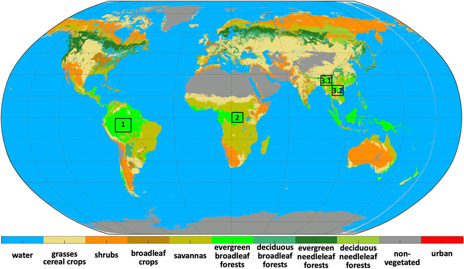
FIGURE 1. DSCOVR EPIC 10 km land cover map (WWW-VESDR 2021) on Robinson projection with Center meridian at 20°E. Our study area includes Amazonian central rainforest (Region 1: 0°–10°S and 70°–60°W), Congo rainforests (Region 2: 5°S–5°N and 20°–30°E) and Southeast Asian rainforest (Region 3.1: 23.50°–26.57°N and 92.5°–98.62°E; Region 3.2: 19.80°–21.54°N and 97.93°–105°E). Our study areas are depicted as squares, which are part of evergreen broadleaf forests.

About 95% of our Amazonian central rainforest is covered with terra firme rainforests (Nepstad et al., 1994). The average annual rainfall during the 2000–2019 period is about 2,600 mm. The seasonal cycle consists of a short dry season, June to October, and a long wet season thereafter.

The equatorial rainforests of Central Africa are the second largest and least disturbed of the biodiversly-rich and highly productive rainforests on Earth (Cook et al., 2020). Our study area includes central and part of western and northeast Congolian lowland forests. The Congo basin exhibits bimodal precipitation pattern and has two wet and two dry seasons per year (Yang et al., 2015). The wet seasons occur in March-April-May and September-October-November, while dry season months are December-January-February and June-July-August. The average annual rainfall over the past 2 decades is about 1761 mm.

Our third region consists of two sub-regions depicted as Region 3.1 (23.50–26.57°N and 92.5–98.62°E) and 3.2 (19.80–21.54°N and 97.93–105°E). The first one is a subtropical moist broadleaf forest ecoregion in Mizoram–Manipur–Kachin rain forests. It occupies the lower hillsides of the mountainous border region joining India, Bangladesh, and Burma (Myanmar). The average annual rainfall over the past 20 years is about 1,545 mm. The dry season is from October to April, and wet season is May to September. Region 3.2 represents a subtropical moist broadleaf forest ecoregion in Northern Indochina. The wet seasons occur in May to September while dry season months are October to April.

Data Used

Various variables from several independent satellite sensors over our study area were used in this research. These include land cover maps and leaf area index (LAI) from the MODerate resolution Imaging Spectroradiometer (MODIS), precipitation from Tropical Rainfall Measuring Mission (TRMM), surface bidirectional reflectance factor (BRF) from Multi-angle Imaging SpectroRadiometer (MISR) on the Terra platform and BRF from Earth Polychromatic Imaging Camera (EPIC) on Deep Space Climate Observatory (DSCOVR).

MODIS land cover dataset. Collection 6 Terra and Aqua MODIS land cover product from 2001 to 2019 at yearly temporal frequency and 0.05° spatial resolution (Friedl and Sulla-Menashe 2015) was used to identify our study area. This product provides several classification schemes. The map of LAI classification scheme was adopted in this research. Figure 2 illustrates LAI classification scheme used by DSCOVR EPIC operational algorithm for the generation of Vegetation Earth System Data Record (WWW-VESDR 2021).

FIGURE 2

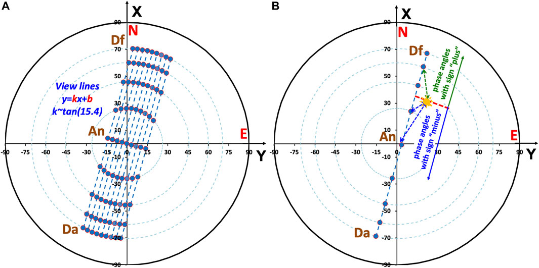
FIGURE 2. MISR observing geometry. Here the X and Y axes point toward the North and East, respectively. (A) Directions from ground pixel to MISR cameras form view lines on the polar plane, each characterizing by slope, k, and intercept, b. (B) Sun-sensor geometry is parametrized in terms the solar zenith angle (SZA), intercept b and phase angle (PA), the latter is the angle between the directions to the Sun and sensor. We assign the sign “plus” to the phase angle if the MISR view direction approaches the direction to the sun from North (i.e., above the dotted red line perpendicular to the MISR view line), and “minus” otherwise.

MODIS LAI datasets. Collection 6 Terra and Aqua MODIS LAI products (Myneni et al., 2015a; Myneni et al., 2015b) for the period February 2000 to December 2019 were used in this study. The LAI dataset provides 8-days composite LAI at 500-m spatial resolution. The C6 MODIS LAI product was evaluated against ground-based measurements of LAI and through inter-comparisons with other satellite LAI products (Yan et al., 2016; Yan et al., 2016).

TRMM precipitation dataset. Monthly precipitation data from the TRMM (3B43 version 7) at 0.25° spatial resolution for the period January 2000 to December 2019 (WWW-TRMM 2011) was used in this study. This dataset provides the best-estimate precipitation rate and root-mean-square precipitation-error estimates by combining four independent precipitation fields (Huffman et al., 2007).

DSCOVR EPIC MAIAC dataset. Level 2 DSCOVR EPIC Multi-Angle Implementation of Atmospheric Correction (MAIAC, version 1) surface BRF and aerosol optical depth (AOD) at 551 nm from 2016 to 2019 were also used. The EPIC instrument has provided imageries in near backscattering directions with the phase angle between 4° and 12° at ten ultra-violet to near infrared (NIR) narrow spectral bands until June 27, 2019, when the spacecraft was placed in an extended safe hold due to degradation of the inertial navigation unit (gyros). DSCOVR returned to full operations on March 2, 2020 after the navigation problem had been resolved. After March 2020 the range of phase has substantially increased towards backscattering reaching 2° (Lyapustin et al., 2021; Marshak et al., 2021).

The MAIAC BRF are available at four spectral bands; they are 433 (band width 3.0) nm, 551 (3.0) nm, 680 (2.0) nm and 780 (2.0) nm. Data are projected on a 10-km SIN grid and available at 65–110 min temporal frequency (WWW-MAIAC 2018). EPIC sees Amazonian rainforests between 11 UTC and 18 UTC, Congo forests between 5 UTC and 14 UTC and Southeast Asian rainforests between 1 and 7 UTC.

MISR datasets. The MISR sensor views each 1.1 km ground pixel symmetrically about the nadir in the forward and aftward directions along the spacecraft’s flight track. Image data are acquired with nominal view zenith angles relative to the surface reference ellipsoid of 0.0⁰ (camera An), 26.1⁰ (Af and Aa), 46.5⁰ (Bf and Ba), 60.0⁰ (Cf and Ca) and 70.5⁰ (Df and Da) in four spectral bands centered at 446 (band width 41.9 nm), 558 (28.6) nm, 672 (21.9) nm, and 866 (39.7) nm. MISR obtains global coverage between ±82° latitudes in 9 days (Diner et al., 1998; Diner et al., 1999). Level 2 version 3 MISR land surface (WWW-MISR_SURFACE 1999) and aerosol (WWW-MISR_AEROSOL 1999) products for the period of January 2016 to December 2019 over our study area were used. The surface reflectance parameter BRF in 9 view angles and four MISR spectral bands is at 1.1 km spatial resolution. The aerosol optical depth is available at 4.4 km spatial resolution. Both parameters are projected on Space Oblique Mercator (SOM) projection, in which the reference meridian nominally follows the spacecraft ground track.

Directions from ground pixel to MISR cameras form view lines on the polar plane, which are characterized by slope, $k=\tan {\upsilon }_K$, and intercept, b (Figure 2A). The slope is aligned with ground track and is roughly constant with ${\upsilon }_K\approx 15.5°$. The intercept is associated with location of pixel within the MISR 360 km swath. We parameterize MISR BRF in terms of the solar zenith angle, phase angle and intercept. The phase angle, $\gamma$, is calculated as

$\gamma ={\text{acosΩΩ}}_0=\text{acos}\left(\cos \theta \cos {\theta }_0+\sin \theta \sin {\theta }_0\cos \left(\phi -{\phi }_0\right)\right) ,(5)$

where ${\text{Ω}}_0\sim ({\theta }_0,{\phi }_0)$ and $\text{Ω}\sim (\theta ,\phi )$ are directions from ground pixel to the Sun and sensor, respectively. We assign the sign “plus” to the phase angle if the MISR view direction approaches to the direction to the Sun from North, i.e., $\sin \theta \cos \left({\upsilon }_K-\phi \right)>\sin {\theta }_0\cos ({\upsilon }_K-{\phi }_0)$, and “minus” otherwise (Figure 2B).

Data Processing

The MODIS LAI and TRMM precipitation data over forested pixels were selected using flags indicating highest retrieval quality. The 8-days 500 m LAI products over our study area (Figure 1) were spatially aggregated to 0.01° and 0.1° resolutions which were then used in our analyses.

The MISR and DSCOVR EPIC surface BRF over our study area were first refined by removing pixels with aerosol optical depth over 0.3. MISR and EPIC datasets were further re-projected to 0.01° and 0.1° Climate Modeling Grids (CMG), respectively. For each pixel, MISR and EPIC DASFs were calculated using Eq. 2, which then were used to generate monthly DASFs. If there were several observations of a pixel within a given month, a median DASF value was assigned to such pixel.

Area-averaged DASF as a function of mean SZA and phase angle, $\gamma$, is defined as

$DASF\left(SZA,\gamma \right)=\frac{{{\displaystyle \sum }}_{xy\in A}DAS{F}_{xy}\left(SZ{A}_{xy},VZ{A}_{xy}\right)\cos SZ{A}_{xy}}{{{\displaystyle \sum }}_{xy\in A}\cos SZ{A}_{xy}} ,(6)$

where the summation is over pixels $(x,y)$ in the selected area A at which the phase angle takes a given value $\gamma$.

Hot Spot Parameter and Effective Extinction Coefficient

Equation 4 is used to simulate DASF. It depends on the hot spot parameter, h, and effective extinction coefficient, L. The former is a function of SZA and determines the angular shape of DASF, while the latter controls its magnitude and depends on LAI. The following two-step fitting technique was implemented to derive equations for h and L using monthly MISR DASF.

Step 1: Matching angular shapes of observed and modeled DASF. For a given month, we used $SZ{A}_{xy}$ and monthly average MODIS LAI as a first approximation to the effective extinction coefficient (i.e., $L_{xy}\approx LA{I}_{xy}$) to simulate $DAS{F}_{xy}$ at each pixel $(x,y)$ in MISR view angles as a function of h. Next, we used Eq. 6 to calculate area-averaged simulated-DASF as a function of hot spot parameter, h. Finally, we selected h that minimized ${(R^2-1)}^2+{(s-1)}^2$, where $R^2$ and s are the coefficient of determination and slope of the relationship between area averaged values of observed and simulated DASFs. The selected hot spot parameter provides the best agreement between angular shapes of modeled and observed DASF.

Step 2: Matching magnitudes of observed and modeled DASF. For a given month, we used SZA and h (SZA) to simulate $DAS{F}_{xy}$ at MISR view angles as a function of L. Eq. 6 was used to calculate area averaged simulated-DASF as a function of effective extinction coefficient, L, i.e., ${\overline{DASF}}_{mod}\left(\gamma ,L\right)$. We selected L that minimizes Normalized Root Mean Square Error (NRMSE) between simulated, ${\overline{DASF}}_{mod}$, and observed, ${\overline{DASF}}_{MISR}$, area-averaged DASFs, i.e.,

$NRMSE\left(L\right)=\frac{\sqrt{\frac{1}{N}{{\displaystyle \sum }}_{\gamma }{\left[{\overline{DASF}}_{mod}\left(\gamma ,L\right)-{\overline{DASF}}_{MISR}\left(\gamma \right)\right]}^2}}{\frac{1}{N}{{\displaystyle \sum }}_{\gamma }{\overline{DASF}}_{MISR}\left(\gamma ,L\right)} \to min. (7)$

This value of L matches magnitudes of observed and modelled DASFs.

Monthly MISR DASF data for the 2017 to 2019 period over our study area (Figure 1) were used to execute our two-step fitting procedure. The SZA exhibits small variation within our regions during a month and therefore can be accurately represented by its monthly mean. A time series of the solutions to the Step-1 procedure therefore gives a set of the hot spot parameters corresponding to different SZA. Seasonal variations of LAI in equatorial forests allowed us to accumulate solutions to the Step-2 procedure corresponding to different values of MODIS LAI. We used those sets to derive dependences of the hot spot parameter and effective extinction coefficient on SZA and LAI, respectively.

Figure 3 shows an example of our two-step fitting technique for Congo forests (region 2) in September-2018. As illustrated in Figure 4, Eq. 4 approximates observed DASF to within NRMSE = 8% and R² = 0.85. The largest difference between observed and simulated DASFs occurred at phase angles above 90⁰. Such points are separated by an ellipse in Figure 4. For PA > 90⁰, MISR BRFs were mainly acquired by off-nadir F and D cameras, which have higher uncertainties compared to near nadir observations.

FIGURE 3

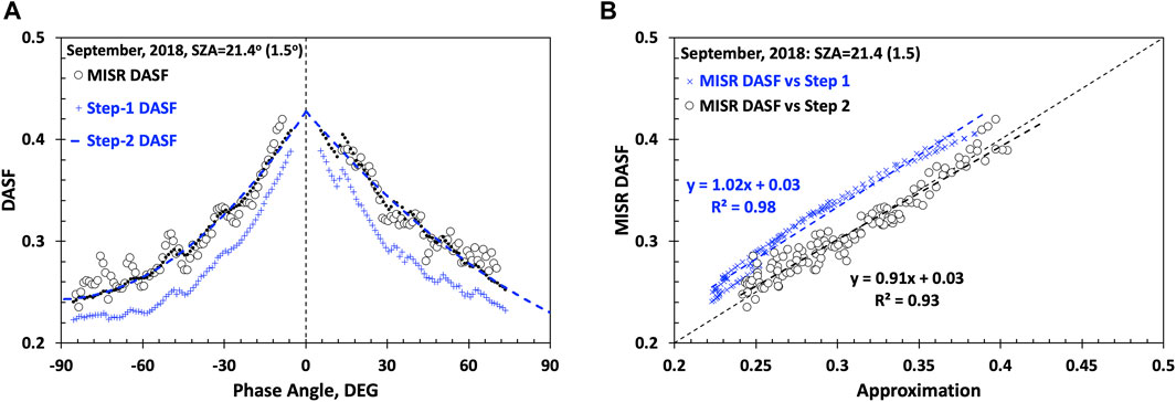
FIGURE 3. (A) MISR DASF of region 2 (Congo forests) in September-2018 (hollow circles). Its step-1 and step-2 approximations are shown as crosses and dots, respectively. The dashed line is a polynomial fit to the Step-2 approximation. (B) MISR DASF versus step-1 (crosses) and step-2 (circles) approximations. NRMSEs between MISR DASF and its Step 1 and Step 2 approximations are 12 and 4%, respectively. Mean SZA (std) = 21.2⁰ (1.5⁰), h = 0.8, LAI = 5.6, L = 7.15.

FIGURE 4

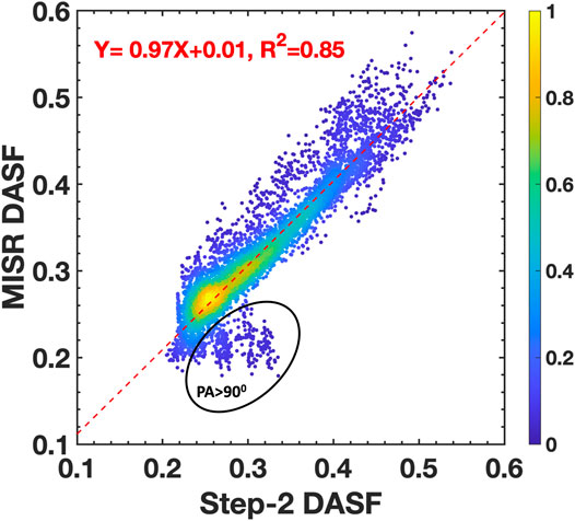
FIGURE 4. MISR DASF vs. its Step-2 approximation accumulated over our study area during the 2017 to 2019 period. NRMSE = 8%; R² = 0.85. The ellipse separates values of DASF at Phase Angles (PA) above 90⁰.

The sets of solutions to the Steps 1 and 2 procedures allowed us to regress the hot spot parameter, h, and effective extinction coefficient, L, versus SZA and MODIS LAI, respectively, as (Figure 5)

$h\left(SZA\right)=5.96-5.90\cos SZA\approx 11.92{\sin }^2\frac{SZA}{2},(8)$

$L=2.93\cdot LA{I}_{MODIS}-8.53(9)$

There was no correlation between L and SZA, as expected.

FIGURE 5

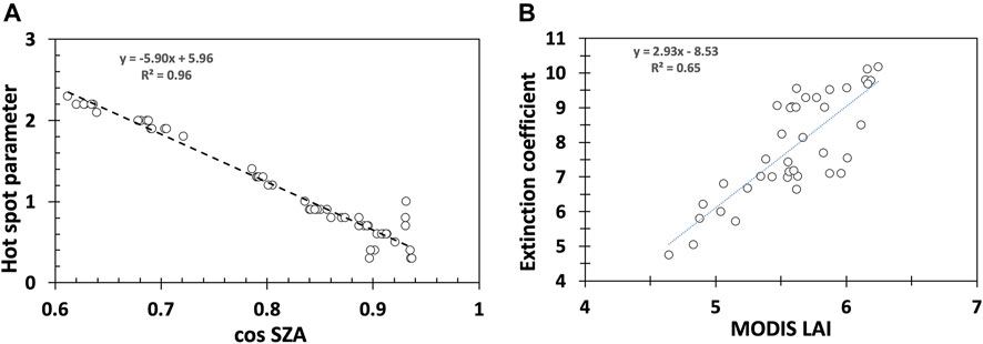
FIGURE 5. (A). Hot spot parameter h vs. cos (SZA). (B) The effective extinction coefficient vs MODIS LAI derived from monthly MISR DASF for the period between 2017 and 2019.

Thus, our model for DASF of equatorial forests is generated by Eq. 4 with the hot spot parameter h and effective extinction coefficient L given by Eqs 8, 9. It has two input parameters; they are Sun position in the sky, ${\text{Ω}}_0\sim ({\theta }_0,{\phi }_0)$, and MODIS LAI.

Results

Assessment of DASF

Observed versus modeled DASF. We used monthly MISR DASF for the period between 2017 and 2019 to derive equations for the hot spot parameter and effective extinction coefficient. The proximity between observed and modeled DASFs were characterized by NRMSE = 8%, R² = 0.85 (Figure 4). We analyzed modelled and observed monthly DASF for Year 2016 to see if the performance metrics is similar to that of the training data set. Figure 6 illustrates monthly MISR DASF and its simulated counterpart for Amazonian forests in April 2016. The largest differences between them are at high phase angles. Figure 7 shows MISR DASF plotted versus modeled DASF accumulated over our study area during Year 2016. The comparison suggests a good performance of Eq. 4 to simulate MISR DASF over equatorial forests.

FIGURE 6

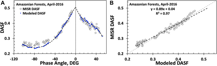
FIGURE 6. (A) MISR DASF of Amazonian forests in April-2016 (hollow circles) and its approximation by Eq. 4 (dots). The dashed line is a polynomial fit to the modeled DASF. (B) MISR DASF vs. modeled DASF. NRMSE = 4%.

FIGURE 7

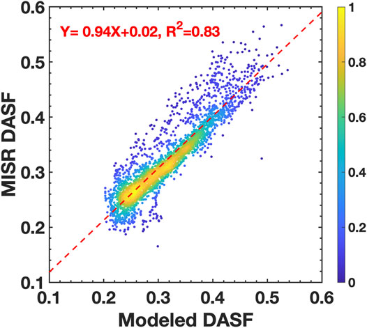
FIGURE 7. MISR DASF vs. its approximation by Eq. 4 accumulated over our study area during Year 2016. NRMSE = 9.2%; R² = 0.83.

Diurnal variations of observed and modeled DASFs. The next step in the assessment of our approach is to see if the model can reproduce diurnal variation of monthly EPIC DASF. Figure 8 shows examples of diurnal variations in observed and modeled DASFs for 3 regions in our study area. As one can see the largest deviation between model and observation occurs when SZA exceeds 60⁰. The uncertainty of the MAIAC BRF product is low for the EPIC observations near the local noon. It however may significantly increase at high zenith angles resulting in an underestimation of surface BRF (Lyapustin et al., 2021). And this is what we see in Figure 8.

FIGURE 8

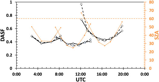
FIGURE 8. Diurnal courses of monthly EPIC DASF (solid line), modeled DASF (dashed line) and SZA (dotted line) for region 3.2 in Southeast Asian (diamonds), Congo (triangles) and Amazonian (circles) forests on 2017-02-24, 2018-06-14 and 2018-07-24, respectively. A SZA level of 60⁰ is shown as a horizontal dashed line. NRMSE values for Southeast Asian, Congo and Amazonian forests are 3.9, 3.6 and 16.3%, respectively. RMSE for Amazonian forests is 3.1% if SZA < 60⁰.

Scatter plot of diurnal courses of modeled and EPIC DASFs accumulated over Amazonian, Congo forests and region 3.2 in southeast Asia during the 2017 to 2019 period is shown in Figure 9. Note that data from December to November over Congo forests are not present in this plot. For these regions, our model approximates diurnal courses of the observed DASFs to within NRMSE = 7% with R² = 0.82.

FIGURE 9

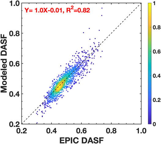
FIGURE 9. Correlation between diurnal courses of modeled and EPIC DASFs accumulated over Amazonian, Congo forests and region 3.2 in southeast Asia during the 2017 to 2019 period. Data from December to February over Congo forests are excluded. NRMSE = 7%. The relationship between these data is characterized by a regression line with a slope of 1 and negligible intercept; R² = 0.82.

On average, modeled DASF over Congo during December through February overestimates observed DASF by about 20%. About 70% of data on the scatter plane are located within a 15% circle centered at mean values of EPIC and modeled DASFs and therefore differ from respective mean values by less than 15%.

For the region 3.1 in Southeast Asian rainforest, modeled DASF overestimates observations by about 5%. The data are also concentrated on the scatter plane: about 75% of data on the model-vs.-observation scatter plane are concentrated within a 15% circle centered at mean values of observed and modeled DASFs. The R² is consequently low (Y = 0.8X+0.08, R² = 0.32).

In summary, Eq. 4 can accurately reproduce DASF in terms of proximity to both angular variations observed by MISR and diurnal courses measured by DSCOVR EPIC sensor. It therefore provides a strong basis for synergy of DSCOVR EPIC and Terra MISR sensors to monitor changes in equatorial forests. Our next step is to see if the model can detect changes.

Monitoring Equatorial Forests

The forest structural organization determines the magnitude and angular variation of DASF (Schull et al., 2011; Knyazikhin et al., 2013). Its angular signatures therefore provide unique and rich sources of diagnostic information about forests. Here we analyze DASF over our study area to see if it can detect seasonal changes of the equatorial forests.

The seasonal transition between wet and dry seasons is a distinct feature of equatorial rainforests, which leads to intra-annual patterns of leaf flushing and abscission (Samanta et al., 2012; Bi et al., 2015). Since our study is focused on structurally intact and undisturbed regions of the equatorial forests (i.e., no changes in forest geometry), variation in leaf area is a key factor causing variation in DASF.

We start with analyses of variation in the DASF acquired over Amazonian central rainforest. In situ studies and satellite data indicated higher leaf area during the dry season relative to the wet season (Huete et al., 2006; Hutyra et al., 2007; Myneni et al., 2007; Hilker et al., 2014; Jones et al., 2014). The growth-limiting impact of water deficit on rainforest during the dry season is alleviated through deep roots and hydraulic redistribution (Oliveira et al., 2005; Pierret et al., 2016), resulting in a sunlight mediated seasonality in leaf area (Bi et al., 2015). Figure 10 illustrates these findings, that is, green leaf area increases during the dry season (June to October), has high values during the early part of the wet season (November to October) and decreases thereafter (March to May).

FIGURE 10

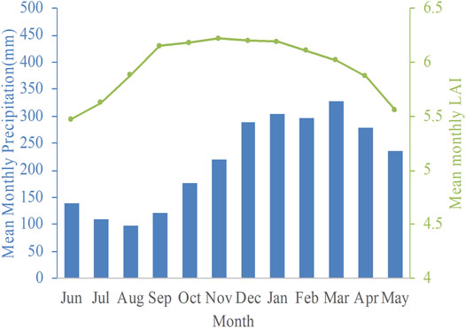
FIGURE 10. Annual courses of monthly-average precipitation and LAI over the Amazonian central rainforest. Monthly data were accumulated over the time period February 2000 to December 2019.

Let us compare observed DASFs from the late dry season (October) and middle part of the wet season (March). Eq. 4 predicts that an increase in the effective extinction coefficient, with SZA unchanged, increases the magnitude of DASF at all phase angles, i.e., results in an upward shift in the angular signature of the DASF, as illustrated in Figure 3. The SZAs in the select region of Amazonian forests in March (SZA = 25.5, std = 1.2) and October (SZA = 20.5, std = 1.1) are very close. At low SZA such a small difference minimally impacts the shape of angular signatures. As one can see in Figure 11, both MISR and EPIC show a distinct decrease in DASF in all phase angles between October and March with no discernible change in the overall shape of the angular signatures. Such a simple change in magnitude can only result from a change in LAI since other structural variables, such as tree crown shape and size do not vary seasonally in this forest.

FIGURE 11

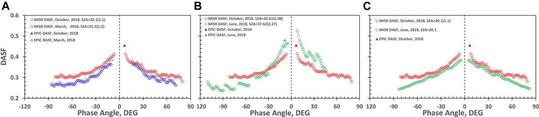
FIGURE 11. Changes in MISR (circles) and EPIC (triangle) DASFs of Amazonian central rainforests from October to March (A), from June to October (B) and transformation of EPIC DASF in June to sun-sensor geometry in March (C). Numbers in parentheses in legends show std of solar zenith angle. Relative difference between MISR and EPIC DASFs is below 8%. Values of NRMSE between MISR DASF and its modeled counterpart do not exceed 9%.

Let us now consider DASF in the early (June) and late (October) dry seasons. LAI has changed from about 5.5 to 6.4. MISR and EPIC measurements are made at significantly higher SZA in June (SZA = 37.6, std = 2.3) compared to October (SZA = 20.6, std = 1.1). The magnitude and shape of angular signatures are impacted when both canopy properties and SZA vary as middle panel in Figure 11 illustrates. This makes the comparison of the signatures difficult. We can transform the June’s signature to the sun-sensor geometry in October using Eq. 4. As right panel of Figure 11 demonstrates the transformed DASF is a downward shift of the October’s DASF, indicating a lower LAI in June. DASFs of the remining regions in our study area exhibit similar behavior (not shown here).

Our next example demonstrates time series of DSCOVR EPIC DASF acquired over the Congolese forests. The Congo basin exhibits bimodal precipitation pattern and has two wet and two dry seasons per year (Yang et al., 2015). The wet seasons occur in March -April-May and September-October-November, while dry season months are December to February and June to August. Unlike Amazonian forests, monthly average LAI follow the patterns of precipitation (Figure 12). It exhibits notable bimodal seasonal variations.

FIGURE 12

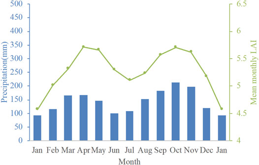
FIGURE 12. Annual courses of monthly-average precipitation and LAI over the Congolese forests. Monthly data were accumulated over the period February 2000 to December 2019.

The above analyses have demonstrated that an increase in LAI, with SZA unchanged, results in an upward shift in the angular signature of the DASF (Figure 3). The EPIC DASF at fixed solar zenith and phase angles therefore should covary with LAI. The Earth-observing geometry of the EPIC sensor is characterized by phase angle between 2⁰ and 12⁰. A question then arises whether or not such small variation in phase angle can be ignored. Therefore, we examine two algorithms to generate EPIC time series. The first one selects EPIC observations at SZA = 25⁰, 30⁰ and 45⁰ irrespective of values of the phase angle. If there are no reflectance data under these illumination conditions during a month, we transform DASF to a desired SZA. In the second case, we select observation at fixed sun-sensor geometries. Figure 13 shows LAI and DASF at fixed SZA = 30⁰ and varying phase angle. At low SZA, the EPIC time series correlates well with the bimodal seasonal variation of LAI, as expected. This also suggests that Eq. 4 is an effective tool to fill missing data at a given fixed SZA.

FIGURE 13

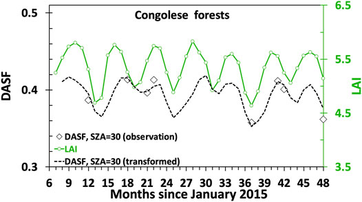
FIGURE 13. Time series of LAI (circles), observed (diamonds) and transformed (dashed line) EPIC DASF at SZA = 30⁰ for the period from 2015 to 2018.

An increase in SZA however can eliminate the bimodal feature of DASF. This is illustrated in Figure 14 showing annual courses of EPIC DASF generated by the two algorithms introduced above. As one can see in left panel of this figure, the EPIC time series at SZA = 45⁰ becomes flat between May and October. Two factors are responsible for this effect. First, the decrease of phase angle to its local minimum in July enhances DASF and therefore tends to suppress decrease in DASF due to the dry season decrease in LAI. At low SZA LAI has a stronger impact on DASF than phase angle. The impact of phase angle however increases with SZA and can become a dominant factor causing variation in DASF. In our example, this occurs at a SZA of 45⁰ and higher. As right panel of Figure 14 illustrates, DASF at fixed SZA and phase angle retains its bimodal property. Thus, both SZA and phase angle should be taken into account when analyzing DSCOVR EPIC data. Eq. 4 therefore becomes of particular importance for analyses of EPIC observations over vegetated land. A strong effect of phase angle on EPIC reflectance was recently documented in (Marshak et al., 2021). Our analyses reinforce this effect.

FIGURE 14

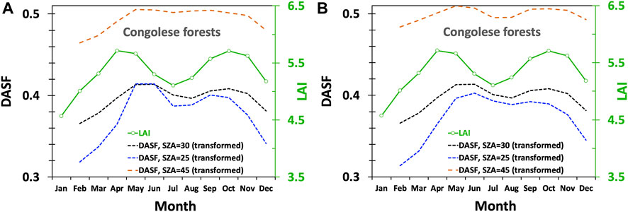
FIGURE 14. Annual courses of LAI and transformed EPIC DASF at SZA = 25⁰, 30⁰ and 45⁰ with (A) varying and (B) fixed phase angles. Monthly data were accumulated over the period 2015 to December 2018.

Summary and Conclusions

We used Directional Area Scattering Function (DASF) to characterize angular signatures of equatorial forests. It describes the canopy BRF if the foliage does not absorb radiation and is a purely structural variable. For vegetation canopies with a dark background, or sufficiently dense vegetation where the impact of canopy background is negligible, the DASF can be accurately approximated from the BRF in the weakly absorbing spectral intervals without involving canopy reflectance models, prior knowledge, or ancillary information regarding leaf scattering properties (Knyazikhin et al., 2013). Equation 2 is used to obtain approximations of DASF from the Terra MISR and DSCOVR EPIC data. The DASF becomes independent on spectral band composition of a sensor acquiring surface reflectance data, which is an important prerequisite for achieving consistency and complementarity between DSCOVR EPIC and Terra MISR observations.

We adapted a model for the canopy hot spot implemented in the operational algorithm for generation of Earth System Data Record (VESDR) from DSCOVR EPIC observations (Yang et al., 2017; WWW-VESDR 2021). In this approach, the sunlit leaves are treated as a stochastic reflecting boundary, which depends on distribution of leaves in the canopy space and the Sun position in the sky. Photons reflected by the boundary can either enter the vegetation canopy or exit it. The shaded leaves represent the interior points. Their interactions with photons are described by a stochastic radiative transfer equation. The directional escape probability that appears in Eq. 1 is a weighted sum of photons reflected by the boundary and canopy interior points. Kuusk’s model of the hot spot incorporated into the extinction coefficient (Supplementary Appendix SA) is used to evaluate the escape probability as a function of scattering order, which is then used to calculate the average escape probability (Supplementary Appendix SB). Contributions of multiple scattered photons are accounted by the recollision probability.

Here we simplified this model. First, a one-dimensional radiative transfer equation is used to simulate canopy radiative regime (Supplementary Appendix SA6). Second, the average escape probability is approximated by a probability calculated for first order scattered photons (Supplementary Appendix SC). Under these assumptions, DASF is approximated by a simple equation that depends on two parameters. They are the hot spot parameter that appears in the canopy hot spot coefficient and the effective extinction coefficient. The former determines the shape of DASF, while the latter controls its magnitude. These two parameters should be specified to generate angular signatures of equatorial forests.

In spite of substantial theoretical advancement in modeling the radiative transfer in vegetation canopies, quantitative data on the hot spot are still few and far between. Here we specified the hot spot parameter by fitting shapes of observed and modeled DASF using MODIS LAI as an initial approximation to the effective extinction coefficient. The hot spot parameter was found to be almost proportional to $1-\cos SZA$ (R² = 0.96) with a coefficient of proportionality around 6 (left panel in Figure 5). The trigonometric term can be interpreted as a correction of the canopy hot spot coefficient (Supplementary Appendix SA4) for errors due to its approximation by a constant value (Supplementary Appendix SA) whereas the coefficient of proportionality as a mean linear dimension of foliage elements (Knyazikhin and Marshak 1991; Nilson 1991) specific to equatorial forests. This equation for the hotspot parameter was used in all our calculations.

The effective extinction coefficient determines the magnitude of the DASF. Theoretically this variable can be obtained by replacing the 3D extinction coefficient with an effective value that provides a best agreement between horizontally averaged canopy reflectances and solutions of 1D radiative transfer equations. Basically, it depends on LAI, leaf normal distributions and clumping indices. In our approach, the effective extinction coefficient was obtained by matching magnitudes of MISR and shape-adjusted modeled DASFs. This coefficient was found to be linearly related to the MODIS LAI (R² = 0.65, right panel in Figure 5). We used this relationship in all our calculations.

Note the MODIS LAI was used as a first approximation to the effective extinction coefficient, which then was iterated to its optimal value. Alternatively, one can use relationships between LAI and various vegetation induces (e.g., NDVI) to make rough estimates of LAI first and then iterate them to the extinction coefficient. This procedure may result in relationships between the extinction coefficient and vegetation indices, which can make the model dependent on the hot spot parameter and vegetation indices.

Our model for angular signatures of equatorial forests can accurately reproduce both MISR angular signatures acquired at 10:30 local solar time and diurnal course of EPIC reflectance (NRMSE<9%, R² > 0.8) and therefore assures consistency and complementarity between DSCOVR EPIC and Terra MISR observations. This provides a powerful tool to argue for changes in vegetation structure as it was demonstrated in our analyses of seasonal variations of angular signatures acquired over equatorial forests.

Data Availability Statement

Publicly available datasets were analyzed in this study. This data can be found here: DSCOVR EPIC and Terra MISR data were obtained from the NASA Langley Research Center Atmospheric Science Data Center (ASDC) (https://epic.gsfc.nasa.gov). The MODIS products were acquired from the Land Processes (LP) Distributed Active Archive Center (DAAC) (https://lpdaac.usgs.gov). TRMM 3B43 data are publicly available from the NASA Goddard Earth Sciences (GES) Data and Information Services Center (DISC) (https://disc.gsfc.nasa.gov).

Author Contributions

YK and RM conceived the project. YK and XN conducted analyses of DSCOVR EPIC and Terra MISR and MODIS data. YK led the writing of manuscript.

Funding

This study was supported by the NASA DSCOVR project under grants 80NSSC19K0762 (YK) and 80NSSC19K0760 (RM). XN was supported by the Chinese Scholarship Council (201906280404).

Conflict of Interest

The authors declare that the research was conducted in the absence of any commercial or financial relationships that could be construed as a potential conflict of interest.

The reviewer AL declared a past co-authorship with one of the author YK to the handling editor.

Publisher’s Note

All claims expressed in this article are solely those of the authors and do not necessarily represent those of their affiliated organizations, or those of the publisher, the editors and the reviewers. Any product that may be evaluated in this article, or claim that may be made by its manufacturer, is not guaranteed or endorsed by the publisher.

Acknowledgments

DSCOVR EPIC and Terra MISR data were obtained from the NASA Langley Research Center Atmospheric Science Data Center (ASDC) (https://epic.gsfc.nasa.gov). The MODIS products were acquired from the Land Processes (LP) Distributed Active Archive Center (DAAC) (https://lpdaac.usgs.gov). TRMM 3B43 data are publicly available from the NASA Goddard Earth Sciences (GES) Data and Information Services Center (DISC) (https://disc.gsfc.nasa.gov.

Supplementary Material

The Supplementary Material for this article can be found online at: https://www.frontiersin.org/articles/10.3389/frsen.2021.766805/full#supplementary-material

Footnotes

¹The phase angle is the angle between the directions to the Sun and sensor

References

Adams, J., Lewis, P., and Disney, M. (2018). Decoupling Canopy Structure and Leaf Biochemistry: Testing the Utility of Directional Area Scattering Factor (DASF). Remote Sensing 10 (12), 1911. doi:10.3390/rs10121911

CrossRef Full Text | Google Scholar

Bi, J., Knyazikhin, Y., Choi, S., Park, T., Barichivich, J., Ciais, P., et al. (2015). Sunlight mediated seasonality in canopy structure and photosynthetic activity of Amazonian rainforests. Environ. Res. Lett. 10 (6), 064014. doi:10.1088/1748-9326/10/6/064014

CrossRef Full Text | Google Scholar

Brando, P. M., Goetz, S. J., BacciniBeck, A., Nepstad, D. C., Beck, P. S. A., and Christman, M. C. (2010). Seasonal and interannual variability of climate and vegetation indices across the Amazon. Proc. Natl. Acad. Sci. 107 (33), 14685–14690. doi:10.1073/pnas.0908741107

PubMed Abstract | CrossRef Full Text | Google Scholar

Cook, K. H., Liu, Y., and Vizy, E. K. (2020). Congo Basin drying associated with poleward shifts of the African thermal lows. Clim. Dyn. 54 (1), 863–883. doi:10.1007/s00382-019-05033-3

CrossRef Full Text | Google Scholar

Diner, D. J., Asner, G. P., Davies, R., Knyazikhin, Y., Muller, J. P., Nolin, A. W., et al. (1999). New directions in earth observing: Scientific applications of multiangle remote sensing. Bull. Am. Meteorol. Soc. 80 (11), 2209–2228. doi:10.1175/1520-0477(1999)080<2209:NDIEOS>2.0.CO;2

CrossRef Full Text | Google Scholar

Diner, D. J., Beckert, J. C., Reilly, T. H., Bruegge, C. J., Conel, J. E., Kahn, R. A., et al. (1998). Multi-angle Imaging SpectroRadiometer (MISR) instrument description and experiment overview. IEEE Trans. Geosci. Remote Sensing 36 (4), 1072–1087. doi:10.1109/36.700992

CrossRef Full Text | Google Scholar

Féret, J.-B., François, C., Asner, G. P., Gitelson, A. A., Martin, R. E., Bidel, L. P. R., et al. 2008. "PROSPECT-4 and 5: Advances in the leaf optical properties model separating photosynthetic pigments." Remote Sensing Environ. 112 (6):3030–3043. doi:10.1016/J.Rse.2008.02.012

CrossRef Full Text | Google Scholar

Friedl, M., and Sulla-Menashe, D. (2015). “MCD12C1 MODIS/Terra+Aqua Land Cover Type Yearly L3 Global 0.05Deg CMG V006 [Data set],” in NASA EOSDIS Land Processes DAAC. Sioux Falls, South Dakota: USGS Earth Resources Observation and Science (EROS) Center. doi:10.5067/MODIS/MCD12C1.006

CrossRef Full Text | Google Scholar

Gerstl, S. A. W., and Simmer, C. (1986). Radiation physics and modelling for off-nadir satellite-sensing of non-Lambertian surfaces. Remote Sensing Environ. 20 (1), 1–29. doi:10.1016/0034-4257(86)90011-8

CrossRef Full Text | Google Scholar

Goel, N. S., Qin, W., and Wang, B.. 1997 "On the estimation of leaf size and crown geometry for tree canopies from hotspot observations." J. Geophys. Res. 102 (D24):29543–29554. doi:10.1029/97jd01110

CrossRef Full Text | Google Scholar

Gorkavyi, N., Carn, S., DeLand, M., Knyazikhin, Y., Krotkov, N., Marshak, A., et al. (2021). Earth Imaging From the Surface of the Moon with a DSCOVR/EPIC-Type Camera. Front. Remote Sens. 2, 24. doi:10.3389/frsen.2021.724074

CrossRef Full Text | Google Scholar

Hilker, T., Lyapustin, A. I., Tucker, C. J., Hall, F. G, Ranga, B., Myneni, R. B., et al. (2014). Vegetation dynamics and rainfall sensitivity of the Amazon. Proc. Natl. Acad. Sci. USA 111 (45), 16041–16046. doi:10.1073/pnas.1404870111

PubMed Abstract | CrossRef Full Text | Google Scholar

Huang, D., Knyazikhin, Y., Dickinson, R. E., Rautiainen, M., Stenberg, P., Disney, M., et al. (2007). Canopy spectral invariants for remote sensing and model applications. Remote Sensing Environ. 106 (1), 106–122. doi:10.1016/j.rse.2006.08.001

CrossRef Full Text | Google Scholar

Huang, D., Knyazikhin, Y., Wang, W., Deering, D., Stenberg, P., Shabanov, N., et al. (2008). Stochastic transport theory for investigating the three-dimensional canopy structure from space measurements. Remote Sensing Environ. 112 (1), 35–50. doi:10.1016/j.rse.2006.05.026

CrossRef Full Text | Google Scholar

Huete, A. R., Didan, K., Shimabukuro, Y. E., Ratana, P., Saleska, S. R., Hutyra, L. R., et al. (2006). Amazon rainforests green-up with sunlight in dry season. Geophys. Res. Lett. 33, 6. doi:10.1029/2005GL025583

CrossRef Full Text | Google Scholar

Huffman, G. J., Bolvin, D. T., Nelkin, E. J., Wolff, D. B., Adler, R. F., Gu, G., et al. (2007). The TRMM Multisatellite Precipitation Analysis (TMPA): Quasi-Global, Multiyear, Combined-Sensor Precipitation Estimates at Fine Scales. J. Hydrometeorology 8 (1), 38–55. doi:10.1175/JHM560.1

CrossRef Full Text | Google Scholar

Hutyra, L. R., Munger, J. W., Saleska, S. R., Gottlieb, E., Daube, B. C., Dunn, A. L, et al. (2007). Seasonal controls on the exchange of carbon and water in an Amazonian rain forest. J. Geophys. Res. 112 (G3), a–n. doi:10.1029/2006JG000365

CrossRef Full Text | Google Scholar

Jones, M. O., Kimball, J. S., and Nemani, R. R. (2014). Asynchronous Amazon forest canopy phenology indicates adaptation to both water and light availability. Environ. Res. Lett. 9 (12), 124021. doi:10.1088/1748-9326/9/12/124021

CrossRef Full Text | Google Scholar

Knyazikhin, Y., and Marshak, A. (1991). “Fundamental Equations of Radiative Transfer in Leaf Canopies, and Iterative Methods for Their Solution,” in Photon-vegetation Interactions: applications in plant physiology and optical remote sensing. Editors R. B. Myneni, and J. Ross (Berlin Heidelberg: Springer-Verlag), 9–43. doi:10.1007/978-3-642-75389-3_2

CrossRef Full Text | Google Scholar

Knyazikhin, Y., Schull, M. A., Stenberg, P., Mottus, M., Rautiainen, M., Yang, Y., et al. (2013). Hyperspectral remote sensing of foliar nitrogen content. Proc. Natl. Acad. Sci. 110 (3), E185–E192. doi:10.1073/pnas.1210196109

PubMed Abstract | CrossRef Full Text | Google Scholar

Knyazikhin, Y., Schull, M. A., Xu, L., Myneni, R. B., and Samanta, A. (2011). Canopy spectral invariants. Part 1: A new concept in remote sensing of vegetation. J. Quantitative Spectrosc. Radiative Transfer 112 (4), 727–735. doi:10.1016/j.jqsrt.2010.06.014

CrossRef Full Text | Google Scholar

Kuusk, A. (1991). “The Hot Spot Effect in Plant Canopy Reflectance,” in Photon-vegetation Interactions: applications in plant physiology and optical remote sensing. Editors R. B. Myneni, and J. Ross (Berlin Heidelberg: Springer Berlin Heidelberg), 139–159. doi:10.1007/978-3-642-75389-3_5

CrossRef Full Text | Google Scholar

Latorre-Carmona, P., Knyazikhin, Y., Alonso, L., Moreno, J. F., Pla, F., and Yang Yan, Y. (2014). On Hyperspectral Remote Sensing of Leaf Biophysical Constituents: Decoupling Vegetation Structure and Leaf Optics Using CHRIS-PROBA Data Over Crops in Barrax. IEEE Geosci. Remote Sensing Lett. 11 (99), 1579–1583. doi:10.1109/LGRS.2014.2305168

CrossRef Full Text | Google Scholar

Lewis, P., and Disney, M.. 2007 "Spectral invariants and scattering across multiple scales from within-leaf to canopy." Remote Sensing Environ. 109 (2):196–206. doi:10.1016/J.Rse.2006.12.015

CrossRef Full Text | Google Scholar

Lewis, S. L., Lopez-Gonzalez, G., Sonké, B., Affum-Baffoe, K., Baker, T. R., Ojo, L. O., et al. (2009). Increasing carbon storage in intact African tropical forests. Nature 457 (7232), 1003–1006. doi:10.1038/nature07771

PubMed Abstract | CrossRef Full Text | Google Scholar

Lyapustin, A., Wang, Y., Go, S., Choi, M., Korkin, S., Huang, D., et al. (2021). Atmospheric Correction of DSCOVR EPIC: Version 2 MAIAC Algorithm. Front. Remote Sens. 2, 31. doi:10.3389/frsen.2021.748362

CrossRef Full Text | Google Scholar

Lyapustin, A., Wang, Y., Korkin, S., and Huang, D. (2018). MODIS Collection 6 MAIAC algorithm. Atmos. Meas. Tech. 11 (10), 5741–5765. doi:10.5194/amt-11-5741-2018

CrossRef Full Text | Google Scholar

Marshak, A., Delgado-Bonal, A., and Knyazikhin, Y. (2021). Effect of Scattering Angle on Earth Reflectance. Front. Remote Sens. 2, 22. doi:10.3389/frsen.2021.719610

CrossRef Full Text | Google Scholar

Marshak, A., Herman, J., Adam, S., Karin, B., Carn, S., Cede, A., et al. (2018). Earth Observations from DSCOVR EPIC Instrument. Bull. Am. Meteorol. Soc. 99 (9), 1829–1850. doi:10.1175/bams-d-17-0223.1

PubMed Abstract | CrossRef Full Text | Google Scholar

Marshak, A., and Knyazikhin, Y. (2017). The spectral invariant approximation within canopy radiative transfer to support the use of the EPIC/DSCOVR oxygen B-band for monitoring vegetation. J. Quantitative Spectrosc. Radiative Transfer 191, 7–12. doi:10.1016/j.jqsrt.2017.01.015

PubMed Abstract | CrossRef Full Text | Google Scholar

Martonchik, J. V., Bruegge, C. J., and Strahler., A. H. (2000). A review of reflectance nomenclature used in remote sensing. Remote Sensing Rev. 19 (1-4), 9–20. doi:10.1080/02757250009532407

CrossRef Full Text | Google Scholar

Morton, D. C., Nagol, J., Carabajal, C. C., Rosette, J., Palace, M., Cook, B. D., et al. (2014). Amazon forests maintain consistent canopy structure and greenness during the dry season. Nature 506 (7487), 221–224. doi:10.1038/nature13006

PubMed Abstract | CrossRef Full Text | Google Scholar

Myneni, Ranga. B. (1991). Modeling radiative transfer and photosynthesis in three-dimensional vegetation canopies. Agric. For. Meteorology 55 (3), 323–344. doi:10.1016/0168-1923(91)90069-3

CrossRef Full Text | Google Scholar

Myneni, R. B., Knyazikhin, Y., and Park., T. (2015a). “MOD15A2H MODIS/Terra Leaf Area Index/FPAR 8-Day L4 Global 500m SIN Grid V006 [Data set],” in NASA EOSDIS Land Processes DAAC. Sioux Falls, South Dakota: USGS Earth Resources Observation and Science (EROS) Center. doi:10.5067/MODIS/MOD15A2H.006

CrossRef Full Text | Google Scholar

Myneni, R. B., Knyazikhin, Y., and Park, T. (2015b). “MYD15A2H MODIS/Aqua Leaf Area Index/FPAR 8-Day L4 Global 500m SIN Grid V006 [Data set],” in NASA EOSDIS Land Processes DAAC. Sioux Falls, South Dakota: USGS Earth Resources Observation and Science (EROS) Center. doi:10.5067/MODIS/MYD15A2H.006

CrossRef Full Text | Google Scholar

Myneni, R. B., Yang, W., Nemani, R. R., NemaniDickinson, A. R., Dickinson, R. E., Knyazikhin, Y., et al. (2007). Large seasonal swings in leaf area of Amazon rainforests. Proc. Natl. Acad. Sci. 104 (12), 4820–4823. doi:10.1073/pnas.0611338104

PubMed Abstract | CrossRef Full Text | Google Scholar

Nepstad, D. C., de Carvalho, C. R., Davidson, E. A., Jipp, P. H., Lefebvre, P. A., Negreiros, G. H., et al. (1994). The role of deep roots in the hydrological and carbon cycles of Amazonian forests and pastures. Nature 372 (6507), 666–669. doi:10.1038/372666a0

CrossRef Full Text | Google Scholar

Nilson, T. (1991). “Approximate Analytical Methods for Calculating the Reflection Functions of Leaf Canopies in Remote Sensing Applications,” in Photon-Vegetation Interactions: Applications in Optical Remote Sensing and Plant Ecology. Editors R. B. Myneni, and J. Ross (Berlin, Heidelberg: Springer Berlin Heidelberg), 161–190. doi:10.1007/978-3-642-75389-3_6

CrossRef Full Text | Google Scholar

Oliveira, R. S., Dawson, T. E., and Burgess, D. C. (2005). Hydraulic redistribution in three Amazonian trees. Oecologia 145 (3), 354–363. doi:10.1007/s00442-005-0108-2

PubMed Abstract | CrossRef Full Text | Google Scholar

Pan, Y., Birdsey, R. A., Fang, J., Houghton, R., Kauppi, P. E., Kurz, W. A., et al. (2011). A Large and Persistent Carbon Sink in the World's Forests. Science 333 (6045), 988–993. doi:10.1126/science.1201609

PubMed Abstract | CrossRef Full Text | Google Scholar

Pierret, A., Maeght, J.-L., Clément, C., Montoroi, J.-P., Hartmann, C., and Gonkhamdee, S. (2016). Understanding deep roots and their functions in ecosystems: an advocacy for more unconventional research. Ann. Bot. 118 (4), 621–635. doi:10.1093/aob/mcw130

PubMed Abstract | CrossRef Full Text | Google Scholar

Pisek, J., Arndt, S. K., Erb, A., Pendall, E., Schaaf, C., Wardlaw, T. J., et al. (2021). Exploring the Potential of DSCOVR EPIC Data to Retrieve Clumping Index in Australian Terrestrial Ecosystem Research Network Observing Sites. Front. Remote Sens. 2, 6. doi:10.3389/frsen.2021.652436

CrossRef Full Text | Google Scholar

Qin, W., Gerstl, S. A. W., Deering, D. W., and Goel, N. S. (2002). Characterizing leaf geometry for grass and crop canopies from hotspot observations: A simulation study. Remote Sensing Environ. 80 (1), 100–113. doi:10.1016/S0034-4257(01)00291-7

CrossRef Full Text | Google Scholar

Qin, W., Goel, N. S., and Wang., B. (1996). The hotspot effect in heterogeneous vegetation canopies and performances of various hotspot models. Remote Sensing Rev. 14 (4), 283–332. doi:10.1080/02757259609532323

CrossRef Full Text | Google Scholar

Reichstein, M., Bahn, M., Ciais, P., Frank, D., Mahecha, M. D., Seneviratne, S. I., et al. (2013). Climate extremes and the carbon cycle. Nature 500 (7462), 287–295. doi:10.1038/nature12350

PubMed Abstract | CrossRef Full Text | Google Scholar

Ross, J. K., and Marshak, A. L.. 1988 "Calculation of canopy bidirectional reflectance using the Monte Carlo method." Remote Sensing Environ. 24 (2):213–225. doi:10.1016/0034-4257(88)90026-0

CrossRef Full Text | Google Scholar

Ross, J., and Marshak, A. (1991). Influence of the Crop Architecture Parameters on Crop Brdf - a Monte-Carlo Simulation. Phys. Measurements Signatures Remote Sensing 1 (2319), 357–360.

Google Scholar

Ross, Juhan. (1981). The radiation Regime and Architecture of Plant Stands. The Hague: Dr. W. Junk.

Google Scholar

Saleska, S. R., Didan, K., Huete, A. R., and da Rocha, H. R. (2007). Amazon Forests Green-Up during 2005 Drought. Science 318 (5850), 612. doi:10.1126/science.1146663

PubMed Abstract | CrossRef Full Text | Google Scholar

Saleska, S. R., Wu, J., Guan, K., Araujo, A. C., Huete, A., Nobre, A. D., et al. (2016). Dry-season greening of Amazon forests. Nature 531 (7594), E4–E5. doi:10.1038/nature16457

PubMed Abstract | CrossRef Full Text | Google Scholar

Samanta, A., Costa, M. H., Nunes, S. A., Xu, L., and Myneni, R. B. (2011). Comment on "Drought-Induced Reduction in Global Terrestrial Net Primary Production from 2000 through 2009". Science 333 (6046), 1093. doi:10.1126/science.1199048

PubMed Abstract | CrossRef Full Text | Google Scholar

Samanta, A., Ganguly, S., Hashimoto, H., Devadiga, S., Vermote, E., Knyazikhin, Y., et al. (2010). Amazon forests did not green-up during the 2005 drought. Geophys. Res. Lett. 37 (5), a–n. doi:10.1029/2009GL042154

CrossRef Full Text | Google Scholar

Samanta, A., Knyazikhin, Y., Xu, L., Dickinson, R. E., Fu, R., Costa, M. H., et al. (2012). Seasonal changes in leaf area of Amazon forests from leaf flushing and abscission. J. Geophys. Res. 117. doi:10.1029/2011jg001818

CrossRef Full Text | Google Scholar

Schaepman-Strub, G., Schaepman, M. E., Painter, T. H., Dangel, S., and Martonchik, J. V.. 2006 "Reflectance quantities in optical remote sensing-definitions and case studies." Remote Sensing Environ. 103 (1):27–42. doi:10.1016/J.Rse.2006.03.002

CrossRef Full Text | Google Scholar

Schlesinger, W. H., and Bernhardt, E. S. (2012). Biogeochemistry: An Analysis of Global Change. 3 ed. Cambridge: Academic Press.

Google Scholar

Schull, M. A., Knyazikhin, Y., Xu, L., Samanta, A., Carmona, P. L., Lepine, L., et al. (2011). Canopy spectral invariants, Part 2: Application to classification of forest types from hyperspectral data. J. Quantitative Spectrosc. Radiative Transfer 112 (4), 736–750. doi:10.1016/j.jqsrt.2010.06.004

CrossRef Full Text | Google Scholar

Smolander, S., and Stenberg, P. (2005). Simple parameterizations of the radiation budget of uniform broadleaved and coniferous canopies. Remote Sensing Environ. 94 (3), 355–363. doi:10.1016/J.Rse.2004.10.010

CrossRef Full Text | Google Scholar

Song, W., Knyazikhin, Y., Wen, G., Marshak, A., Mõttus, M., Yan, K., et al. (2018). Implications of Whole-Disc DSCOVR EPIC Spectral Observations for Estimating Earth's Spectral Reflectivity Based on Low-Earth-Orbiting and Geostationary Observations. Remote Sensing 10 (10), 1594. doi:10.3390/rs10101594

CrossRef Full Text | Google Scholar

Stenberg, P., Mõttus, M., and Rautiainen, M. (2016). Photon recollision probability in modelling the radiation regime of canopies - A review. Remote Sensing Environ. 183, 98–108. doi:10.1016/j.rse.2016.05.013

CrossRef Full Text | Google Scholar

Vladimirov, V. S. (1963). Mathematical problems in the one-velocity theory of particle transport, Vol. AECL-1661. Clark River, Ontario: Atomic Energy of Canada Limited.

Google Scholar

WWW-MAIAC (2018). “DSCOVR EPIC L2 Multi-Angle Implementation of Atmospheric Correction (MAIAC), Version 01,” in NASA Langley Atmospheric Science Data Center DAAC. doi:10.5067/EPIC/DSCOVR/L2_MAIAC.001

CrossRef Full Text | Google Scholar

WWW-MISR_AEROSOL (1999). “MISR Level 2 Aerosol parameters V003,” in NASA Langley Atmospheric Science Data Center DAAC. https://asdc.larc.nasa.gov/project/MISR/MIL2ASAE_3.

Google Scholar

WWW-MISR_SURFACE (1999). “MISR Level 2 Surface parameters V003,” in NASA Langley Atmospheric Science Data Center DAAC. doi:10.5067/TERRA/MISR/MIL2ASLS_L2.003-23

CrossRef Full Text | Google Scholar

WWW-TRMM (2011). “Tropical Rainfall Measuring Mission (TRMM) (2011), TRMM (TMPA/3B43) Rainfall Estimate L3 1 month 0.25 degree x 0.25 degree V7,” in Goddard Earth Sciences Data and Information Services Center (GES DISC). 10.5067/TRMM/TMPA/MONTH/7.

Google Scholar

WWW-VESDR (2021). “DSCOVR EPIC Level 2 Vegetation Earth System Data Record (VESDR), Version 2,” in NASA Langley Atmospheric Science Data Center DAAC. doi:10.5067/EPIC/DSCOVR/L2_VESDR.002

CrossRef Full Text | Google Scholar

Xu, L., Samanta, A., Costa, M. H., Ganguly, S., Nemani, R. R., and Myneni, R. B. (2011). Widespread decline in greenness of Amazonian vegetation due to the 2010 drought. Geophys. Res. Lett. 38 (7), a–n. doi:10.1029/2011GL046824

CrossRef Full Text | Google Scholar

Yan, K., Park, T., Yan, G., Chen, C., Yang, B., Liu, Z., et al. (2016). Evaluation of MODIS LAI/FPAR Product Collection 6. Part 1: Consistency and Improvements. Remote Sensing 8 (5), 359. doi:10.3390/rs8050359

CrossRef Full Text | Google Scholar

Yan, K., Park, T., Yan, G., Liu, Z., Yang, B., Chen, C., et al. (2016). Evaluation of MODIS LAI/FPAR Product Collection 6. Part 2: Validation and Intercomparison. Remote Sensing 8 (6), 460. doi:10.3390/rs8060460

CrossRef Full Text | Google Scholar

Yang, B., Knyazikhin, Y., Mõttus, M., Rautiainen, M., Stenberg, P., Yan, L., et al. (2017). Estimation of leaf area index and its sunlit portion from DSCOVR EPIC data: Theoretical basis. Remote Sensing Environ. 198, 69–84. doi:10.1016/j.rse.2017.05.033

PubMed Abstract | CrossRef Full Text | Google Scholar

Yang, W., Seager, R., Cane, M. A., and Lyon, B. (2015). The Annual Cycle of East African Precipitation. J. Clim. 28 (6), 2385–2404. doi:10.1175/JCLI-D-14-00484.1

CrossRef Full Text | Google Scholar