 Lei Chen
 Zhiyong Xu1
 Zhao Zhao
- 1School of Electronic and Optical Engineering, Nanjing University of Science and Technology, Nanjing, China
- 2Nonresident Senior Faculty Fellow, Center for Global Soundscapes, Purdue University, West Lafayette, IN, United States
In recent years, passive acoustic monitoring (PAM) has become increasingly popular. Many acoustic indices (AIs) have been proposed for rapid biodiversity assessment (RBA), however, most acoustic indices have been reported to be susceptible to abiotic sounds such as wind or rain noise when biotic sound is masked, which greatly limits the application of these acoustic indices. In this work, in order to take an insight into the influence mechanism of signal-to-noise ratio (SNR) on acoustic indices, four most commonly used acoustic indices, i.e., the bioacoustic index (BIO), the acoustic diversity index (ADI), the acoustic evenness index (AEI), and the acoustic complexity index (ACI), were investigated using controlled computational experiments with field recordings collected in a suburban park in Xuzhou, China, in which bird vocalizations were employed as typical biotic sounds. In the experiments, different signal-to-noise ratio conditions were obtained by varying biotic sound intensities while keeping the background noise fixed. Experimental results showed that three indices (acoustic diversity index, acoustic complexity index, and bioacoustic index) decreased while the trend of acoustic evenness index was in the opposite direction as signal-to-noise ratio declined, which was owing to several factors summarized as follows. Firstly, as for acoustic diversity index and acoustic evenness index, the peak value in the spectrogram will no longer correspond to the biotic sounds of interest when signal-to-noise ratio decreases to a certain extent, leading to erroneous results of the proportion of sound occurring in each frequency band. Secondly, in bioacoustic index calculation, the accumulation of the difference between the sound level within each frequency band and the minimum sound level will drop dramatically with reduced biotic sound intensities. Finally, the acoustic complexity index calculation result relies on the ratio between total differences among all adjacent frames and the total sum of all frames within each temporal step and frequency bin in the spectrogram. With signal-to-noise ratio decreasing, the biotic components contribution in both the total differences and the total sum presents a complex impact on the final acoustic complexity index value. This work is helpful to more comprehensively interpret the values of the above acoustic indices in a real-world environment and promote the applications of passive acoustic monitoring in rapid biodiversity assessment.
1 Introduction
Biodiversity assessment is an increasingly urgent task in the face of global environmental change (Pereira et al., 2013; Bradfer-Lawrence et al., 2020). Despite ambitious global targets to reduce biodiversity loss (Tittensor et al., 2014), pressure on biodiversity has increased notably (Butchart et al., 2010; Dröge et al., 2021) over the past four decades. Quantifying biological diversity is fundamental for setting priorities for conservation (Mittermeier et al., 1998; Brooks et al., 2006), especially in the current period of dramatic biodiversity loss (Brooks et al., 2006; Ceballos et al., 2015; Cifuentes et al., 2021). Traditionally, this has relied on detailed species inventories, which however often require an extensive, costly sampling effort, especially in high-biodiversity areas (Cifuentes et al., 2021).
Passive acoustic monitoring, a promising alternative to conducting point-count surveys, may offer a more rapid and economical means of terrestrial biodiversity appraisal than traditional methods in situ surveys (Pijanowski, 2011). There are two main advantages associated with acoustic monitoring. One is the ability to collect data simultaneously across large areas with minimal observer bias (Deichmann et al., 2018; Gibb et al., 2019). Another advantage is that data collection can be carried out over a long period of time with minimum disturbance to wildlife (Deichmann et al., 2018; Gibb et al., 2019; Shamon et al., 2021).
In recent years, a number of acoustic indices (AIs) have been developed for rapid, automated assessments of ecosystem conditions or as a proxy for richness and/or diversity (Gasc et al., 2013a; Rajan et al., 2019; Sugai and Llusia, 2019; Shamon et al., 2021). Several studies have reported relationships between different AIs and measures of species richness and/or diversity, in which conclusions with regard to the “best” performing index differ between ecosystems (Fuller et al., 2015; Gasc et al., 2015; Fairbrass et al., 2017; Mammides et al., 2017; Myers et al., 2019; Zhao et al., 2019). These uncertainties warrant ecosystem-specific assessments of the performance of AIs (Gasc et al., 2015). Furthermore, there are still some open questions concerning AIs, which include the impact of various abiotic sounds (such as wind, rain, and road noise), the sensitivity of AIs to different signal-to-noise ratio (SNR) conditions, and the optimized usage of AIs in acoustic monitoring. For instance, when using AIs to quantify the complexity of an acoustic community, it is necessary to consider the influence on the AIs’ values from variations of SNR in the recording.
Since the varying distance between vocalizing organisms and acoustic recorders inevitably impacts the SNR in the recording, we investigated potential associations between AIs and SNR in this work using field recordings collected in a suburban park in Xuzhou, China. Considering that it is very difficult to ensure the SNR as expected in the survey environment, controlled computational experiments were conducted and different SNR conditions were used. Experimental results suggested that, in addition to different sound unit shapes (Zhao et al., 2019), variations in SNR also contributed to the differences in AIs’ values.
The objective of this study is to take an insight into the influence mechanism of SNR on four most commonly used AIs, i.e., the bioacoustic index (BIO) (Boelman et al., 2007), the acoustic diversity index (ADI) (Villanueva-Rivera et al., 2011), the acoustic evenness index (AEI) (Villanueva-Rivera et al., 2011), and the acoustic complexity index (ACI) (Pieretti et al., 2011). Furthermore, we also presented preliminary ideas to improve the robustness of these AIs, which will be explored in the future.
2 Materials and methods
2.1 Study area
We obtained acoustic recordings from two sites in Jiuli Lake National Wetland Park (Figure 1), located in the northwest of Xuzhou, Jiangsu Province, China (34°19′27′′ - 34°20′44″N, 117°6′2′′ - 117°7′22″E). There are many species of insects, reptiles, anurans, birds (about 42 species), and mammals in the park. Currently, this area is surrounded by densely urbanized infrastructure with a road running through the park.
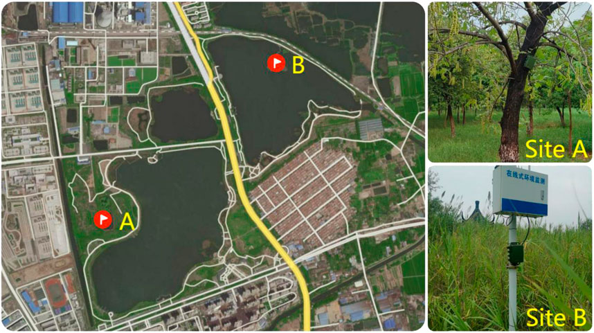
FIGURE 1. Locations of acoustic recorders in Jiuli Lake National Wetland Park, Xuzhou, Jiangsu Province, China. Site A represents a terrestrial sampling point, and site B is surrounded by the lake.
2.2 Data collection
Sound files were recorded at two locations in the park as shown in Figure 1. Site A (34°19′44″N - 117°6′17″E) was 50 m away from the trail and surrounded by trees whilst site B (34°20′18″N - 117°6′54″E) was located on an island in the middle of the lake.
In each of the two locations, we used a SongMeter digital recording device (model SM4, Wildlife Acoustics Inc., Concord, MA) to obtain bird sounds during three consecutive days in each month from June to August of 2022. The recorders were programmed to operate 24 h every day. Recordings were made in wav files (48 kHz sampling rate, 26 dB microphone gain, 16 bits) with 60-min duration each. In this way, for each location, we obtained 72 60-min recordings per month, corresponding to 144 h/month (2 locations × 72 h per point) and 432 h in total.
Figure 2 shows the spectrogram of a 30-s recording as a representative example collected in site A from 6:35:16 a.m. to 6:35:46 a.m. on 24 June 2022. The recording contains various bird sounds with mild winds, and there are almost no obvious anthropogenic sounds. Specifically, one can observe that frequencies below 400 Hz are filled by noise, and between 400 and 12,000 Hz exist rich biological sounds. Here, in line with our previous studies (Zhao et al., 2017; 2019; Zhang et al., 2018), we considered a call or a syllable as an acoustic event. We selected five common and widespread bird species in Xuzhou, of which the vocalizations correspond to five unique sound unit shapes. More specifically, these five sound unit shapes are constant frequency (CF), frequency modulated whistles (FM), broadband pulses (BP), broadband with varying frequency components (BVF), and strong harmonics (SH) (Brandes, 2008). The detailed description of the avian acoustic events used in this work is provided in Table 1. We extracted acoustic events using the same automatic segmentation procedure presented in Zhao et al. (2017). The duration of each event is less than 1 s, facilitating the following experiments.
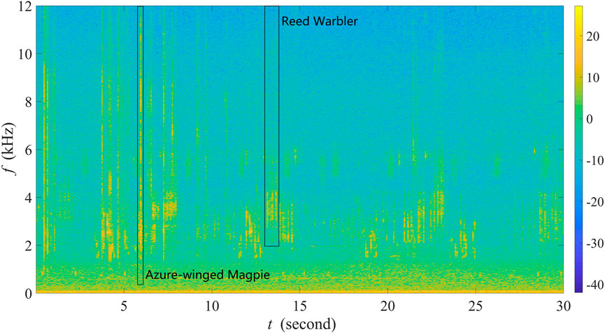
FIGURE 2. Spectrogram of a 30-s recording as a representative example collected in site A at Jiuli Lake National Wetland Park, Xuzhou, Jiangsu Province, China.
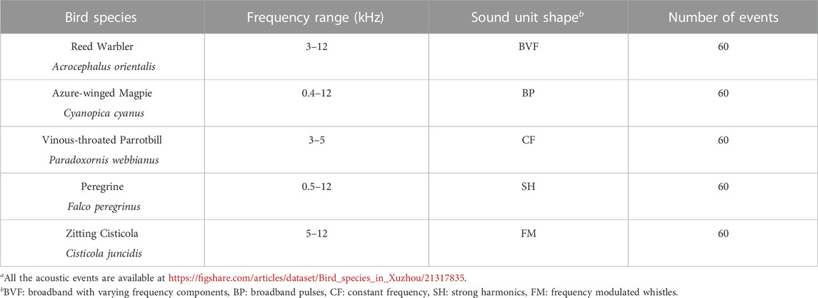
TABLE 1. Details of species and acoustic events used in this work. The five species are common and widespread in Xuzhou. All the acoustic eventsa were extracted from our field recordings.
2.3 Data analysis
We calculated four different indices, i.e., BIO, ACI, ADI, and AEI, using the R programming language version 3.4.2. More specifically, the above indices were computed using the bioacoustic_index, acoustic_complexity, acoustic_diversity, and acoustic_evenness functions, respectively, in the “soundecology” package (Villanueva-Rivera and Pijanowski, 2016). For BIO, the minimum frequency and maximum frequency were set to 0.4 kHz and 12 kHz, respectively. In the case of ACI, the maximum frequency was set to 12 kHz. ADI and AEI were calculated using 12 kHz as the maximum frequency and 1 kHz as the frequency bandwidth (−50 dBFS threshold was used). After all indices’ results were calculated, descriptive statistics (mean, standard deviation) were produced for each index in Experiment 1.
2.4 Experiments
2.4.1 Experiment 1—The effect of SNR
In order to inspect the influence of SNRs on AIs’ values, we focused on vocalization intensity options of acoustic events in this experiment. Using the five bird species listed above (Table 1), we randomly selected six acoustic events of each species, i.e., 30 events in total, and overlaid them on a 1-min background noise recording with each event within every non-overlapping 2 seconds. The background recording was obtained from 5:15 a.m. to 5:16 a.m. on Jun. 24, 2022, at Jiuli Lake National Wetland Park, Xuzhou, Jiangsu Province, China, and the corresponding spectrogram is shown in Figure 3. This recording contained almost no audible sounds but mild winds, providing an acoustic background in natural conditions similar to that in most field recordings. It is worth mentioning that the background noise contains most energy in low frequency range rather than equally distributed across the frequency spectrum.
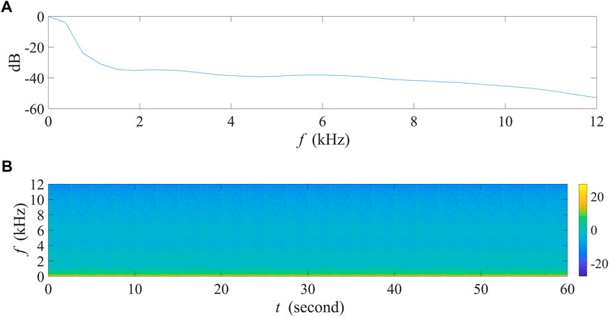
FIGURE 3. The 1-min background noise recording collected at site A in Jiuli Lake National Wetland Park, Xuzhou, Jiangsu Province, China. (A) The normalized power spectrum of the recording. (B) The spectrogram of the recording.
It is well known that the SNR is calculated by the ratio between the average power of the signal and noise. In this work, we multiplied the signal (i.e., the acoustic event) power by a factor a while maintaining the noise power constant, which would result in the desired SNR. Note that although all selected events have high SNRs, the Wiener filter (Arslan, 2006) was further employed upon each event to reduce background noise before constructing experimental recordings.
In this experiment, the SNR of each acoustic event was set to 11 different values, i.e., 35 dB, 30 dB, 25 dB, 20 dB, 15 dB, 10 dB, 5 dB, 0 dB, −5 dB, −10 dB, and −15 dB, resulting in 11 cases total. For each case, 300 random runs were conducted to obtain a statistically significant result, in which all events were set to the same SNR. In each run, we used a random selection of acoustic events without replacement. It is noteworthy that the place of each event within every non-overlapping 2 seconds was also random—that is, considering a certain event (viewed as a 1-s space) and a 2-s space (say, 0–2 s), the event could be placed within 0–1 s or 0.4 s –1.4 s, etc. Finally, each acoustic index was calculated based on the experimental recording. In this way, we conducted 3,300 random runs in total for each of the four acoustic indices.
2.4.2 Experiment 2—Influence mechanism analysis of SNR
In this experiment, we investigated the underlying influence mechanism of SNR on AIs. We selected six acoustic events from each of the 5 bird species listed in Table 1 and the SNR for each acoustic event was set to 35 dB and 0 dB, respectively, representing high and low SNR cases. Similar to experiment 1, the Wiener filter was also employed upon each event to reduce background noise before constructing experimental recordings. For each case, after the total 30 acoustic events were ready, they were overlaid on the same 1-min background recording with each event within every non-overlapping 2 s. It is important to remark that the place of each event within every non-overlapping 2 s was fixed in the two cases to assure that SNR was the only varying factor during the experiment, facilitating the influence mechanism analysis associated with SNR. Finally, for each of the four acoustic indices, the calculation results were based on the experimental recording.
3 Results and discussion
3.1 Experiment 1
As is shown in Figure 4, explicit influence from SNR can be observed on all four indices. Specifically, AEI values were in the opposite direction as SNR decreased. As for the other three indices, their values increased when the SNR was from low to high. Furthermore, when SNR was larger than 0 dB, only BIO values obviously tended towards a constant value.
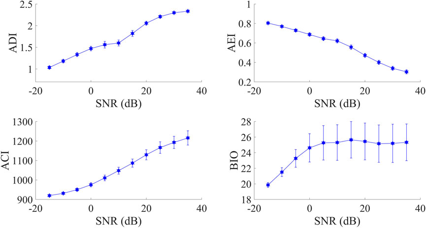
FIGURE 4. The relationship of four acoustic indices with varying SNR. The points represent the mean and the error-bars represent the standard deviation.
3.2 Experiment 2
3.2.1 ADI and AEI
The ADI is obtained from a matrix of frequency bins within a specified frequency range and their respective amplitude values. Then, the proportion of amplitude values above a certain threshold is calculated and the Shannon entropy index is applied to these values, i.e.,
where pi is the fraction of sound in each i-th frequency band in S frequency bands. As for AEI, when pi is ready, the Gini index is applied to the values, yielding
The threshold used for the above two indices is 50 dB below the peak value by default (Villanueva-Rivera et al., 2011). It is worth remarking that the peak value (i.e., the strongest time-frequency bin) is assumed to be dominated by biotic sound in the calculation. However, the peak value in the spectrogram may correspond to abiotic sound when SNR decreases to a certain extent, leading to erroneous results of the proportion of sound occurring in each frequency band when calculating ADI and AEI.
In order to provide an intuitionistic demonstration associated with the aforementioned SNR influence, Figures 5A, B present the signal waveforms under 0 dB and 35 dB SNR conditions, respectively. The corresponding spectrograms are also shown in Figures 5C, D, in which each red dot marks the position of the time-frequency bin with the strongest power.
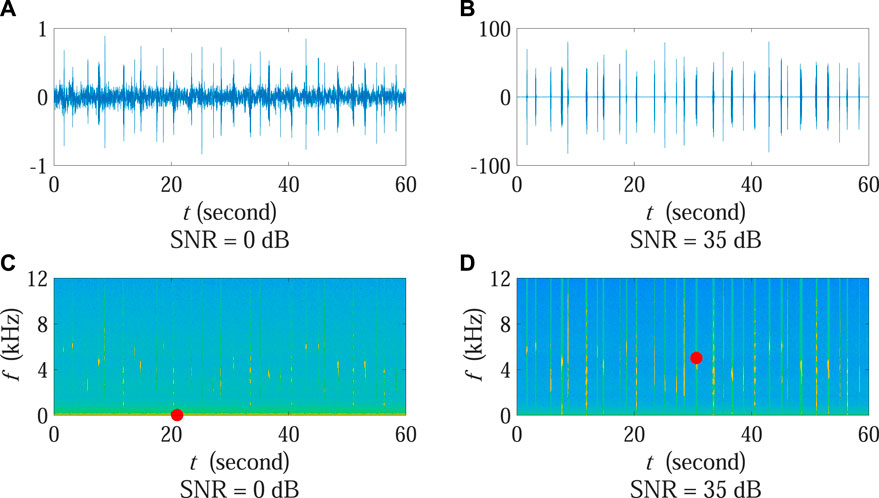
FIGURE 5. Waveforms and spectrograms under the two cases in Experiment 2 when calculating ADI and AEI. (A,B) present the signal waveforms under 0 dB and 35 dB SNR conditions, respectively. The corresponding spectrograms are shown in (C,D). Each red dot marks the position of the time-frequency bin with the strongest power. Note that the amplitude scale of (A) is different from (B).
It can be observed that the position of the time-frequency bin with the strongest power changed obviously at different SNR conditions. Specifically, when the SNR was high, the position was located at the time-frequency bin corresponding to birds (red dot in Figure 5D). Most of time-frequency bins stronger than the threshold were associated with biotic sound and can be correctly used for ADI and AEI computation. In such case, the ADI value was able to reflect the acoustic diversity of the monitoring area with the AEI value reporting the acoustic evenness situation. Nonetheless, under the low SNR condition, the position moved to a noise-dominated bin (red dot in Figure 5C) since the environmental noise in the low frequency zone became protruding as compared with relatively weak biotic sound. This implied that a large number of time-frequency bins corresponding to low frequency noise were selected for ADI and AEI calculation in which the number of bins associated with expected biotic sound considerably decreased at the same time. Consequently, the fraction values of sound within each frequency band across all frequency bands were more unbalanced in Eqs. 1, 2, leading to decreasing ADI and increasing AEI results as is shown in Figure 4.
3.2.2 BIO
BIO is calculated as the area under the curve defined as the difference between the sound level within each frequency band and the minimum sound level, i.e.,
where Si is the sound level of the i-th frequency band in dB, Smin is the minimum value of the sound level among all frequency bands, Δf is the width of frequency band, and N is the number of frequency bands ranging from the minimum frequency fmin to maximum frequency fmax.
Theoretically, Smin in Eq. 3 is expected to represent the sound level of the noise-dominated spectrum. As is shown in Figure 6, the sound level of the background noise spectrum gradually decreased with increasing frequency (black points). When the SNR was high, Smin corresponded to the sound level of the noise spectrum (purple dot) just as expected, and the difference between Si and Smin only contained biotic components. However, under the low SNR condition, Smin moved to the frequency band composed of much weak biotic sound plus noise (green dot), implying that a large amount of noise components were incorrectly included in the calculation. Furthermore, it is also worth mentioning that the value of Si dropped dramatically when the SNR declined (red points in Figure 6 as compared with blue points), so that the accumulation in Eq. 3 decreased accordingly, which could explain the BIO curve in Figure 4.
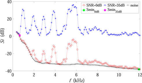
FIGURE 6. Influence mechanism analysis concerning BIO in Experiment 2. The red and blue points represent the sound level of each frequency band for the experimental recording under 0 dB and 35 dB SNR conditions, respectively. The green and purple dots mark the minimum values of the sound level in 0 dB and 35 dB SNR conditions, respectively. The black points denote the sound level of the background noise spectrum, which was fixed in Experiment 2.
3.2.3 ACI
In the ACI calculation, the recording is divided into several temporal steps. In a single temporal step, the summation of the differences between temporally adjacent amplitude values is first computed for each frequency bin and then divided by the total sum of those amplitude values. The ACI result of each temporal step is obtained by the accumulation across frequency bins, yielding
where
Conventionally, biological sound and noise are uncorrelated. The intensity registered in each time-frequency bin can be considered as a composition of two parts, i.e., biotic components and noise components. In this way, the sum of absolute difference, i.e., the numerator in Eq. 4, can be approximately considered to be composed of the biological intensity difference and the noise intensity difference, while the sum of intensity, i.e., the denominator in Eq. 4, can be regarded as the total sum of biological intensity and noise intensity. Note that when the background noise is stationary during the recording, the total difference between two adjacent values of noise intensity is eliminated theoretically. Meanwhile, the sum of the noise intensity is unchanged. However, the biotic sound intensity reduces with SNR decreasing (e.g., vocalizing organisms flying away from the recorder), implying that both the total difference of biotic sound intensity and the total sum of biotic sound intensity decrease accordingly.
In order to further demonstrate the influence mechanism associated with varying SNR on ACI, Figures 7A, B present the values of numerator and denominator at each frequency bin within a certain temporal step under 0 dB and 35 dB SNR conditions, respectively. The corresponding quotient at each frequency bin in Eq. 4 is also shown in Figure 7C, where the black and purple points denote the values in 0 dB and 35 dB SNR conditions, respectively.
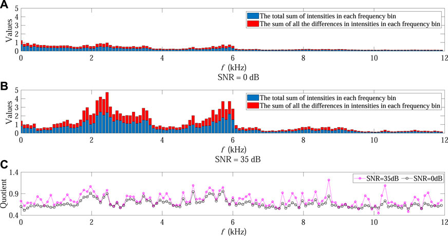
FIGURE 7. Influence mechanism analysis on ACI in Experiment 2. (A,B) present the values of the numerator and denominator at each frequency bin within a certain temporal step under 0 dB and 35 dB SNR conditions, respectively. The red bars represent the total differences in intensities at each frequency bin while the blue bars represent the total sum of intensities at each frequency bin. The corresponding quotient at each frequency bin is shown in (C), where the black and purple points denote the values in 0 dB and 35 dB SNR conditions, respectively.
It can be observed that when the SNR declined the sum of absolute difference in intensities decreased faster than the sum of intensities in almost all frequency bins (black points in Figure 7C as compared with purple points), leading to decreasing ACI value after the accumulation of all quotients along frequency bins in Eq. 4. This could also explain the ACI curve shown in Figure 4.
3.3 Future work
To date, many scholars have mentioned in their works that the AIs values were influenced by geophysical noise and anthropogenic noise (Depraetere et al., 2012; Fairbrass et al., 2017). In general, two simple ways have been employed to reduce the impact when using AIs. One is to use filters to remove low frequency sound from recordings (Depraetere et al., 2012; Towsey et al., 2014a; Pieretti et al., 2015; Bradfer-Lawrence et al., 2020), which could be problematic due to the empirically determined cutoff frequency. The other is to manually or semi-automatically identify and remove the recordings containing biasing sounds (Aide et al., 2013; Gasc et al., 2013b; Rodriguez et al., 2014; Gagne et al., 2022), which could be impractical considering the large volumes of data typically generated by ecoacoustic monitoring (Towsey et al., 2014b).
In practice, since both the background noise level and vocalization intensity may change in the recordings, variation in SNR is almost inevitable. For instance, given a stationary background noise during the monitoring period, vocalizing organisms may move away from the recorder, resulting in decreasing SNR. Alternatively, although vocalizations are produced with fixed intensity as well as the distance to the recorder, varying background noise level also leads to changes in SNR. According to experimental results in Subsection 3.1 that three indices (ADI, ACI, and BIO) decreased while the trend of AEI was in the opposite direction as SNR declined, it should be emphasized that in the context of rapid biodiversity assessment (RBA) that popularly relies on AIs, variation in SNR should be also taken into account when interpreting calculated AIs’ results.
In this work, we analyzed the influence mechanism of SNR on four commonly used AIs. The results presented in the previous section enlightened us with preliminary ideas to improve the robustness of certain AIs. For instance, for ADI and AEI, a fixed detection threshold is commonly used (−50 dBFS as default), which is inappropriate as SNR decreases. A possible improvement may be to use a floating threshold that is adaptive to the noise level to reduce the impact of noise, leading to a more robust detection of biotic sounds. When it comes to BIO, the ambient noise level in each frequency band could be estimated and then can be used to replace Smin in Eq. 3.
Moreover, another idea may be to incorporate microphone array signal processing technique. Theoretically, a microphone array consists of a set of microphones positioned in a way that the spatial information is well captured. Thus, conventional and/or adaptive beamforming methods for spatial filtering in the context of signal enhancement can be employed when the array and AIs are considered in noisy environments. For instance, when the geophysical noise (and/or anthropogenic noise) and biotic sounds concurrently come from different directions, this technique can attenuate noise while keeping the desired signal (i.e., biotic sounds) undistorted, which could be particularly useful in urban areas.
4 Conclusion
Autonomous sound recordings and acoustic indices are regarded as time-efficient assessment tools in the biodiversity conservation context. In this work, four indices (ADI, ACI, AEI, and BIO) were investigated concerning the potential associations between acoustic indices and SNR conditions. Controlled computational experiments were conducted using field recordings collected in a suburban park in Xuzhou, China, in which bird vocalizations were employed as typical biotic sounds. Experimental results suggested that, in addition to different sound unit shapes, variations in SNR also contributed to the differences in AIs values. Furthermore, we analyzed the corresponding influence mechanism of SNR on AIs, based on which we also provided some preliminary ideas for further improvement of AIs’ robustness.
Data availability statement
The datasets presented in this study can be found in online repositories. The names of the repository/repositories and accession number(s) can be found below: https://figshare.com/articles/dataset/Bird_species_in_Xuzhou/21317835.
Author contributions
LC carried out the fieldwork, analyzed the data, and completed the manuscript under guidance. ZX and ZZ conceived the ideas and designed the study. All authors have read and agreed to this submitted version.
Funding
This project was supported by Jiangsu Province Forestry Science and Technology Innovation and Promotion Project (grant number LYKJ-XuZhou[2021]1).
Conflict of interest
The authors declare that the research was conducted in the absence of any commercial or financial relationships that could be construed as a potential conflict of interest.
Publisher’s note
All claims expressed in this article are solely those of the authors and do not necessarily represent those of their affiliated organizations, or those of the publisher, the editors and the reviewers. Any product that may be evaluated in this article, or claim that may be made by its manufacturer, is not guaranteed or endorsed by the publisher.
References
Aide, T. M., Corrada-Bravo, C., Campos-Cerqueira, M., Milan, C., Vega, G., Alvarez, R., et al. (2013). Real-time bioacoustics monitoring and automated species identification. PeerJ 1, e103. doi:10.7717/peerj.103
Arslan, L. (2006). Modified wiener filtering. Signal Process. 86, 267–272. doi:10.1016/j.sigpro.2005.05.021
Boelman, N. T., Asner, G. P., Hart, P. J., and Martin, R. E. (2007). Multi-trophic invasion resistance in Hawaii: Bioacoustics, field surveys, and airborne remote sensing. Ecol. Appl. 17, 2137–2144. doi:10.1890/07-0004.1
Bradfer-Lawrence, T., Bunnefeld, N., Gardner, N., Willis, S. G., and Dent, D. H. (2020). Rapid assessment of avian species richness and abundance using acoustic indices. Ecol. Indic. 115, 106400. doi:10.1016/j.ecolind.2020.106400
Brandes, T. S. (2008). Automated sound recording and analysis techniques for bird surveys and conservation. Bird. Conserv. Int. 18, S163–S173. doi:10.1017/S0959270908000415
Brooks, T. M., Mittermeier, R. A., Da Fonseca, G., Gerlach, J., Hoffmann, M., Lamoreux, J. F., et al. (2006). Global biodiversity conservation priorities. Science 313, 58–61. doi:10.1126/science.1127609
Butchart, S., Walpole, M., Collen, B., van Strien, A., Scharlemann, J., Almond, R., et al. (2010). Global biodiversity: Indicators of recent declines. Science 328, 1164–1168. doi:10.1126/science.1187512
Ceballos, G., Ehrlich, P. R., Barnosky, A. D., García, A., Pringle, R. M., and Palmer, T. M. (2015). Accelerated modern human–induced species losses: Entering the sixth mass extinction. Sci. Adv. 1, e1400253. doi:10.1126/sciadv.1400253
Cifuentes, E., Vélez Gómez, J., and Butler, S. J. (2021). Relationship between acoustic indices, length of recordings and processing time: A methodological test. Biota Colomb. 22. doi:10.21068/c2021.v22n01a02
Deichmann, J. L., Acevedo Charry, O., Barclay, L., Burivalova, Z., Campos Cerqueira, M., D’Horta, F., et al. (2018). It’s time to listen: There is much to be learned from the sounds of tropical ecosystems. Biotropica 50, 713–718. doi:10.1111/btp.12593
Depraetere, M., Pavoine, S., Jiguet, F., Gasc, A., Duvail, S., and Sueur, J. (2012). Monitoring animal diversity using acoustic indices: Implementation in a temperate woodland. Ecol. Indic. 13, 46–54. doi:10.1016/j.ecolind.2011.05.006
Dröge, S., Martin, D. A., Andriafanomezantsoa, R., Burivalova, Z., Fulgence, T. R., Osen, K., et al. (2021). Listening to a changing landscape: Acoustic indices reflect bird species richness and plot-scale vegetation structure across different land-use types in north-eastern Madagascar. Ecol. Indic. 120, 106929. doi:10.1016/j.ecolind.2020.106929
Fairbrass, A. J., Rennett, P., Williams, C., Titheridge, H., and Jones, K. E. (2017). Biases of acoustic indices measuring biodiversity in urban areas. Ecol. Indic. 83, 169–177. doi:10.1016/j.ecolind.2017.07.064
Fuller, S., Axel, A. C., Tucker, D., and Gage, S. H. (2015). Connecting soundscape to landscape: Which acoustic index best describes landscape configuration? Ecol. Indic. 58, 207–215. doi:10.1016/j.ecolind.2015.05.057
Gagne, E., Perez-Ortega, B., Hendry, A. P., Melo-Santos, G., Walmsley, S. F., Rege-Colt, M., et al. (2022). Dolphin communication during widespread systematic noise reduction-a natural experiment amid Covid-19 lockdowns. Front. Remote Sens. 3. doi:10.3389/frsen.2022.934608
Gasc, A., Pavoine, S., Lellouch, L., Grandcolas, P., and Sueur, J. (2015). Acoustic indices for biodiversity assessments: Analyses of bias based on simulated bird assemblages and recommendations for field surveys. Biol. Conserv. 191, 306–312. doi:10.1016/j.biocon.2015.06.018
Gasc, A., Sueur, J., Jiguet, F., Devictor, V., Grandcolas, P., Burrow, C., et al. (2013a). Assessing biodiversity with sound: Do acoustic diversity indices reflect phylogenetic and functional diversities of bird communities? Ecol. Indic. 25, 279–287. doi:10.1016/j.ecolind.2012.10.009
Gasc, A., Sueur, J., Pavoine, S., Pellens, R., and Grandcolas, P. (2013b). Biodiversity sampling using a global acoustic approach: Contrasting sites with microendemics in New Caledonia. PLoS ONE 8, e65311. doi:10.1371/journal.pone.0065311
Gibb, R., Browning, E., Glover-Kapfer, P., and Jones, K. E. (2019). Emerging opportunities and challenges for passive acoustics in ecological assessment and monitoring. Methods Ecol. Evol. 10, 169–185. doi:10.1111/2041-210X.13101
Mammides, C., Goodale, E., Dayananda, S. K., Kang, L., and Chen, J. (2017). Do acoustic indices correlate with bird diversity? Insights from two biodiverse regions in yunnan province, south China. Ecol. Indic. 82, 470–477. doi:10.1016/j.ecolind.2017.07.017
Mittermeier, R. A., Myers, N., Thomsen, J. B., Da Fonseca, G. A. B., and Olivieri, S. (1998). Biodiversity hotspots and major tropical wilderness areas: Approaches to setting conservation priorities. Conserv. Biol. 12, 516–520. doi:10.1046/j.1523-1739.1998.012003516.x
Myers, D., Berg, H., and Maneas, G. (2019). Comparing the soundscapes of organic and conventional olive groves: A potential method for bird diversity monitoring. Ecol. Indic. 103, 642–649. doi:10.1016/j.ecolind.2019.04.030
Pereira, H. M., Ferrier, S., Walters, M., Geller, G. N., Jongman, R. H. G., Scholes, R. J., et al. (2013). Essential biodiversity variables. Science 339, 277–278. doi:10.1126/science.1229931
Pieretti, N., Duarte, M., Sousa-Lima, R. S., Rodrigues, M., Young, R. J., and Farina, A. (2015). Determining temporal sampling schemes for passive acoustic studies in different tropical ecosystems. Trop. Conservation Sci. 8, 215–234. doi:10.1177/194008291500800117
Pieretti, N., Farina, A., and Morri, D. (2011). A new methodology to infer the singing activity of an avian community: The acoustic complexity index (aci). Ecol. Indic. 11, 868–873. doi:10.1016/j.ecolind.2010.11.005
Pijanowski, B. C., Villanueva-Rivera, L. J., Dumyahn, S. L., Farina, A., Krause, B. L., Napoletano, B. M., et al. (2011). Soundscape ecology: The science of sound in the landscape. Bioscience 61, 203–216. doi:10.1525/bio.2011.61.3.6
Rajan, S. C., Athira, K., Jaishanker, R., Sooraj, N. P., and Sarojkumar, V. (2019). Rapid assessment of biodiversity using acoustic indices. Biodivers. Conservation 28, 2371–2383. doi:10.1007/s10531-018-1673-0
Rodriguez, A., Gasc, A., Pavoine, S., Grandcolas, P., Gaucher, P., and Sueur, J. (2014). Temporal and spatial variability of animal sound within a neotropical forest. Ecol. Inf. 21, 133–143. doi:10.1016/j.ecoinf.2013.12.006
Shamon, H., Paraskevopoulou, Z., Kitzes, J., Card, E., Deichmann, J. L., Boyce, A. J., et al. (2021). Using ecoacoustics metrices to track grassland bird richness across landscape gradients. Ecol. Indic. 120, 106928. doi:10.1016/j.ecolind.2020.106928
Sugai, L., and Llusia, D. (2019). Bioacoustic time capsules: Using acoustic monitoring to document biodiversity. Ecol. Indic. 99, 149–152. doi:10.1016/j.ecolind.2018.12.021
Tittensor, D. P., Walpole, M., Hill, S., Boyce, D. G., Britten, G. L., Burgess, N. D., et al. (2014). A mid-term analysis of progress toward international biodiversity targets. Science 346, 241–244. doi:10.1126/science.1257484
Towsey, M., Wimmer, J., Williamson, I., and Roe, P. (2014a). The use of acoustic indices to determine avian species richness in audio-recordings of the environment. Ecol. Inf. 21, 110–119. doi:10.1016/j.ecoinf.2013.11.007
Towsey, M., Zhang, L., Cottman-Fields, M., Wimmer, J., Zhang, J., and Roe, P. (2014b). Visualization of long-duration acoustic recordings of the environment. Procedia Comput. Sci. 29, 703–712. doi:10.1016/j.procs.2014.05.063
Villanueva-Rivera, L. J., and Pijanowski, B. C. (2016). Soundecology: Soundscape ecology. r package. version 1.3.2.
Villanueva-Rivera, L. J., Pijanowski, B. C., Doucette, J., and Pekin, B. (2011). A primer of acoustic analysis for landscape ecologists. Landsc. Ecol. 26, 1233–1246. doi:10.1007/s10980-011-9636-9
Zhang, S.-h., Zhao, Z., Xu, Z.-y., Bellisario, K., and Pijanowski, B. C. (2018). “Automatic bird vocalization identification based on fusion of spectral pattern and texture features,” in 2018 IEEE international conference on acoustics, speech and signal processing (ICASSP), 271–275. doi:10.1109/ICASSP.2018.8462156
Zhao, Z., Xu, Z.-y., Bellisario, K., Zeng, R.-w., Li, N., Zhou, W.-y., et al. (2019). How well do acoustic indices measure biodiversity? Computational experiments to determine effect of sound unit shape, vocalization intensity, and frequency of vocalization occurrence on performance of acoustic indices. Ecol. Indic. 107, 105588. doi:10.1016/j.ecolind.2019.105588
Keywords: acoustic index, rapid biodiversity assessment, passive acoustic monitoring, sound intensity, biodiversity
Citation: Chen L, Xu Z and Zhao Z (2023) Biotic sound SNR influence analysis on acoustic indices. Front. Remote Sens. 3:1079223. doi: 10.3389/frsen.2022.1079223
Received: 25 October 2022; Accepted: 19 December 2022;
Published: 17 January 2023.
Edited by:
Bryan Christopher Pijanowski, Purdue University, United StatesReviewed by:
Luane Stamatto Ferreira, Federal University of Rio Grande do Norte, BrazilGilberto Corso, Federal University of Rio Grande do Norte, Brazil
Copyright © 2023 Chen, Xu and Zhao. This is an open-access article distributed under the terms of the Creative Commons Attribution License (CC BY). The use, distribution or reproduction in other forums is permitted, provided the original author(s) and the copyright owner(s) are credited and that the original publication in this journal is cited, in accordance with accepted academic practice. No use, distribution or reproduction is permitted which does not comply with these terms.
*Correspondence: Zhao Zhao, emhhb3poYW9Abmp1c3QuZWR1LmNu