 Peng-Wang Zhai1*
 Meng Gao2,3
 Bryan A. Franz2
 P. Jeremy Werdell2
 Amir Ibrahim2
 Yongxiang Hu4
 Jacek Chowdhary5,6
- 1Department of Physics, University of Maryland Baltimore County, Baltimore, MD, United States
- 2Ocean Ecology Laboratory, NASA Goddard Space Flight Center, Greenbelt, MD, United States
- 3Science Systems and Applications, Inc., Greenbelt, MD, United States
- 4NASA Langley Research Center, Hampton, VA, United States
- 5NASA Goddard Institute for Space Studies, New York, NY, United States
- 6Department of Applied Physics and Applied Mathematics, Columbia University, New York, NY, United States
A radiative transfer simulator was developed to compute the synthetic data of all three instruments onboard NASA’s Plankton Aerosol, Cloud, ocean Ecosystem (PACE) observatory, and at the top of the atmosphere (TOA). The instrument suite includes the ocean color instrument (OCI), the Hyper-Angular Rainbow Polarimeter 2 (HARP2), and the Spectro-Polarimeter for Planetary Exploration 1 (SPEXone). The PACE simulator is wrapped around a monochromatic radiative transfer model based on the successive order of scattering (RTSOS), which accounts for atmosphere and ocean coupling, polarization, and gas absorption. Inelastic scattering, including Raman scattering from pure ocean water, fluorescence due to chlorophyll, and colored dissolved organic matter (CDOM), is also simulated. This PACE simulator can be used to explore the sensitivity of the hyperspectral and polarized reflectance of the Earth system with tunable atmosphere and ocean parameters, which include aerosol and cloud number concentration, refractive indices, and size distribution, ocean particle microphysical parameters, and solar and sensor-viewing geometry. The PACE simulator is used to study two important case studies. One is the impact of the significant uncertainty in pure ocean water absorption coefficient to the radiance field in the ultraviolet (UV) spectral region, which can be as much as 6%. The other is the influence of different amounts of brown carbon aerosols and CDOM on the polarized radiance field at TOA. The percentage variation of the radiance field due to CDOM is mostly for wavelengths smaller than 600 nm, while brown aerosols affect the whole spectrum from 350 to 890 nm, primarily due to covaried soot aerosols. Both case studies are important for aerosol and ocean color remote sensing and have not been previously reported in the literature.
1 Introduction
NASA’s Plankton, Aerosol, Cloud, and ocean Ecosystem (PACE) mission will carry the Ocean Color Instrument (OCI), which is a hyperspectral scanning radiometer with spectral coverage from the ultraviolet (340 nm) to near-infrared (890 nm) measured at 5 nm spectral resolution with 2.5-nm spectral sampling (Werdell et al., 2019). The 5-nm resolution will better resolve spectral features of some plankton species, as well as atmospheric gas absorption features such as the Oxygen-A band centered near 765 nm. OCI also includes seven shortwave infrared (SWIR) bands centered on 940, 1,038, 1,250, 1,378, 1,615, 2,130, and 2,260 nm, to be used for ocean color atmospheric correction and aerosol and cloud retrievals. In addition, PACE plans to carry two Multi-Angle Polarimeters (MAPs): the Hyper-Angular Rainbow Polarimeter 2 (HARP2) (McBride et al., 2020) and the Spectro-Polarimeter for Planetary Exploration 1 (SPEXone) (Hasekamp et al., 2019). HARP2 will measure the first three Stokes parameters (I, Q, and U) at four wavelengths (441, 549, 669, and 873 nm) and at multiple viewing angles (60 angles for 669 nm, and 10 angles for the other wavelengths) for each pixel. SPEXone will measure the radiance and the Degree of Linear Polarization (DoLP) from 385 to 770 nm with a variable spectral resolution of 2–5 nm for radiance and 10–40 nm for DoLP at five viewing angles, but with less swath coverage than OCI and HARP2. The combined dataset of OCI and the MAPs will provide a plethora of data that will significantly enhance our understanding of the Earth’s ocean, atmosphere, and land systems.
Satellite sensors such as OCI, HARP2, and SPEXone measure radiometric signals at the top of the atmosphere (TOA). Remote sensing algorithms infer environmental variables from the radiometric signals. Over oceans, the environmental variables may include the abundance of aerosols, cloud particles, and hydrosols (in-water particles) and their microphysical properties, many of which are used to infer biogeophysical properties. The radiative transfer model governs the relationship between the environmental variables and radiometric signals, which use the single-scattering properties of particles as inputs. It is imperative to build a satellite sensor simulator based on rigorous radiative transfer models, which conserves the transfer of energy and adequately simulates the interactions between the light and the medium. Rigorous models would allow for understanding the change of radiometric signals in response to variations in the environmental variables needed for developing and testing remote sensing algorithms. The simulator also needs to account for the radiometric characteristics of the sensors, such as the spectral response, so that it can be used as the best representation of the sensor measurements, and which maximizes the benefits of a satellite mission.
In this paper, we report a PACE simulator, which can simulate the hyperspectral radiance that OCI would measure and the polarized signals at multiple wavelengths and multiple viewing angles from HARP2 and SPEXone. The simulator is built around a vector radiative transfer model, which models light multiply scattered in the coupled atmosphere-ocean systems based on the successive order of scattering method (Zhai et al., 2009; Zhai et al., 2010). Plane-parallel geometry is assumed in the radiative transfer model, i.e., we only consider the vertical variation of the optical properties of the atmosphere and ocean. Scattering and absorption due to molecules, aerosols, clouds, and oceanic particles are accurately considered. Gas absorption due to H2O, CO2, O2, CH4, O3, and NO2 are adequately accounted for, which is essential for studying the photon path length distribution in the strong absorbing bands. The model can also simulate inelastic scattering in ocean waters, i.e., Raman scattering by pure waters and fluorescence due to chlorophyll and colored dissolved organic matter (CDOM) (Zhai et al., 2015; Zhai et al., 2017b; Zhai et al., 2018). The detailed system configuration and algorithm are described in Section 2.
Previously, the Global Ocean Physical-Biogeochemical Model (Gregg and Rousseaux, 2017) was developed, which can generate a proxy of global distributions of spectral water leaving radiances based on the spatial distribution of ocean components from the global ocean circulation model. As a result, approximations have been used in the radiative transfer process in the ocean. Our simulator aims to represent all properties of the radiation field in both the atmosphere and ocean as accurately as possible, which preserves both the angular dependence of the light field and the polarization properties.
Two applications of the PACE simulator are presented in the result section. One is a sensitivity study on the impacts of the uncertainty of the spectral absorption coefficient of pure seawater in the ultraviolet (UV) on the radiance field at TOA. The absorption coefficient of pure seawater in the UV is poorly characterized, with values that vary by two orders of magnitude within the literature (Lee et al., 2015; Mason et al., 2016; Twardowski et al., 2018). This uncertainty will significantly impact ocean color remote sensing in the UV once the OCI data is available. The other study is on the convoluted influences of aerosols and CDOM on both radiance and degree of linear polarization at TOA. In particular, both brown carbon and CDOM spectral absorption coefficients increase exponentially as wavelength decreases in the UV. The similarity of the spectral variation of these two components of the atmosphere and ocean system has created great challenges in quantifying their abundances. This paper reports our sensitivity study on different amounts of brown carbon aerosols (Mok et al., 2016) as well as CDOM (Twardowski et al., 2004) to the radiance field using our new PACE simulator, which is a novel contribution to the remote sensing field.
This paper is organized as the following: Section 2 describes the theoretical background of the various elements of this PACE simulator; Section 3 covers the two sensitivity studies in the UV we performed using the PACE simulator; Section 4 provides the discussion.
2 Theoretical Background
2.1 Atmospheric and Ocean Optical Properties
2.1.1 Atmospheric Components
The description of radiative transfer processes in the atmosphere needs vertical profiles of scattering and absorbing particles to be properly defined as inputs. The atmospheric particles include molecules, as well as aerosol, and cloud particles. The default profiles of molecules in the PACE simulator are based upon the US standard atmosphere (1976), but other profiles can easily be substituted by using input files with the same data format. The profile data include the total number density of atmospheric molecules and the volume mixing ratios of the significant absorbers (H2O, CO2, O2, CH4, O3, and NO2) in the UV-SWIR spectral range. The scattering cross-section and the depolarization ratio are a function of wavelength, temperature, and pressure, which we calculate using the algorithm of Tomasi et al. (2005). The molecular scattering cross-section is multiplied by the total number density and integrated over height to obtain the optical depths due to molecular scattering in each discretized vertical layer. We use the Rayleigh scattering matrix, which depends on the depolarization ratio for characterizing molecular scattering (Hovenier et al., 2004).
The scattering matrices of aerosols or clouds can be calculated by the Mie theory for spherical particles (Mishchenko et al., 2002) or other more flexible methods for non-spherical particles, for instance, the finite-difference time-domain method (Yang and Liou, 1996; Sun et al., 2017), the T-matrix method (Mishchenko et al., 2002; Bi and Yang, 2014), and discrete dipole approximation (Yurkin and Hoekstra, 2011). The scattering matrices from different components (molecules, aerosols, and cloud particles) can be weighted by their scattering optical depth in a discretized vertical layer, i.e.,:
where
where
The extinction optical depth
where
The gas absorption optical depth
2.1.2 Ocean Components
The ocean is bounded by the air-sea interface, with its surface roughness parameterized in terms of wind speed (Cox and Munk, 1954). The ocean body is assumed to be a mixture of pure seawater, phytoplankton particles, and their derivative non-algal particles, and CDOM. The Einstein–Smoluchowski phase function is adopted to represent scattering by pure seawater (Mobley, 1994). The scattering coefficient of seawater is a function of salinity and temperature based on Zhang and Hu (2009). In this paper we have used the salinity of 37‰ and temperature of 20
Figure 1 shows the absorption coefficient from the three sources between 300 and 550 nm. MCF is smaller than both IOC and LEE, especially in the UV. The shortest wavelength in the LEE dataset is 350 nm, below which we use the same values as in IOC. The large discrepancy we see in Figure 1 imposes significant uncertainties in ocean color remote sensing in the UV. Section 3 reports a sensitivity study of the TOA radiance due to this discrepancy, which helps quantify the error in future remote sensing algorithms of ocean color in the UV.
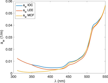
FIGURE 1. The absorption coefficients of pure water from the three sources: IOC, LEE, and MCF.
The spectral absorption coefficient
where
The spectral backscattering coefficient
where the free parameter
Another option to parameterize
The phase function of the phytoplankton particle is determined by the backscattering fraction
where
where
CDOM in our model is assumed to be absorbing only, i.e., the scattering coefficient of CDOM is zero. The absorbing coefficient of CDOM is modeled as:
where
Figure 2 shows the CDOM absorption coefficients as a function of wavelength for [Chla] = 0.03 mg/m3 and [Chla] = 0.1 mg/m3 calculated by using MG2009 and MAG2007 with
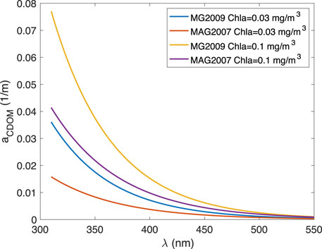
FIGURE 2. The absorption coefficient of CDOM as a function of wavelength for two [Chla] values: 0.03 mg/m3 and 0.3 mg/m3
We also have an option to include the scattering and absorption by sediments following Ibrahim et al. (2016) and Zhai et al. (2017a), which we will not emphasize in this paper.
2.2 Monochromatic Vector Radiative Transfer Model (RTSOS)
The core of the PACE simulator is a monochromatic radiative transfer model based on the successive order of scattering method (RTSOS) (Zhai et al., 2009; Zhai et al., 2010). This model was recently validated in a comprehensive comparison and testbed study (Chowdhary et al., 2020). The atmospheric and ocean optical properties as a function of wavelength is provided as input to RTSOS to calculate the polarized radiance field at user specified locations. The total radiance field is denoted by
where
For the scattering functions with a large forward peak, we implemented several truncation methods to increase the efficiency and maintain the accuracy, including the Delta-M method (Wiscombe, 1977),
To simulate inelastic scattering processes in ocean waters, the excitation radiation field is obtained by looping elastic RTSOS over the excitation wavelengths to evaluate the inelastic source function at the emission wavelength (Zhai et al., 2015; Zhai et al., 2017b). The chlorophyll fluorescence quenching processes can be modeled by allowing the quantum yield, and the fraction of photons reemitted in the total number of photons absorbed by chlorophyll molecules, to vary with the instantaneous photosynthetically available radiation (IPAR) (Morrison and Goodwin, 2010). For more details on how inelastic scattering is implemented in the radiative transfer model, readers are referred to Zhai et al. (2015), Zhai et al. (2017a).
2.3 Double-k Method for Simulating Intra-band Spectral Response
The PACE simulator calls RTSOS in each instrument channel to simulate the radiance field at the center wavelength at a specified location and viewing direction. For channels with little or weak gas absorption, an averaged gas absorption optical depth
where
In some strong absorption bands of gases, such as the Oxygen-A band centered at 765 nm, the absorption cross-section can vary by several orders of magnitude within the full width at half maximum (FWHM) of the considered channel. The approximation made in Eqs 10, 11 will introduce a significant error that cannot be tolerated. In this case, we adopt the philosophy of the double-k method (Duan et al., 2005) to model the monochromatic radiance in a channel by:
where
where the integration limit
where
3 Simulation Results
In this section we present two novel sensitivity studies to show the capabilities of our PACE simulator. The first one is the impact of the uncertainty of pure ocean water absorption coefficients on the radiance field at TOA. In ocean color remote sensing, this is the essential baseline knowledge needed before obtaining information on other constituents. As we showed in Section 2.1.2, there is a large discrepancy in pure water absorption coefficients in the UV. Understanding the variation of the TOA radiance field due to this uncertainty will help the remote sensing community better quantify and interpret derived biogeophysical and bio-optical products. In the second sensitivity study, we check the influences of different amounts of brown carbon aerosols in the atmosphere and CDOM in the ocean to the TOA polarized reflectance to explore how one can address the difficulty of separating the two signals. OCI and SPEXone will cover the UV spectral region, where both brown carbon aerosols and CDOM have increased absorption as wavelength decreases. Brown carbon aerosols are essential for evaluating the radiative forcing balance in the Earth system, while CDOM is critical for ocean carbon cycle studies. It is important to separate two signals and quantify them.
3.1 Variation of the TOA Radiance Field due to the Uncertainty of the Pure Water Absorption Coefficient in the UV
The PACE simulator is used to simulate the spectral TOA reflectance,
Figures 3A,B show the TOA reflectance at nadir as a function of wavelength for [Chla] = 0.03 mg/m3 and 0.1 mg/m3, respectively. FWHM of 5 nm is used in the simulation. Figure 3C shows the percentage differences of the reflectances calculated with LEE and IOC with respect to those with MCF for [Chla] = 0.03 mg/m3. Figure 3D is the same as Figure 3C except for [Chla] = 0.1 mg/m3. It can be seen that the impact of the different
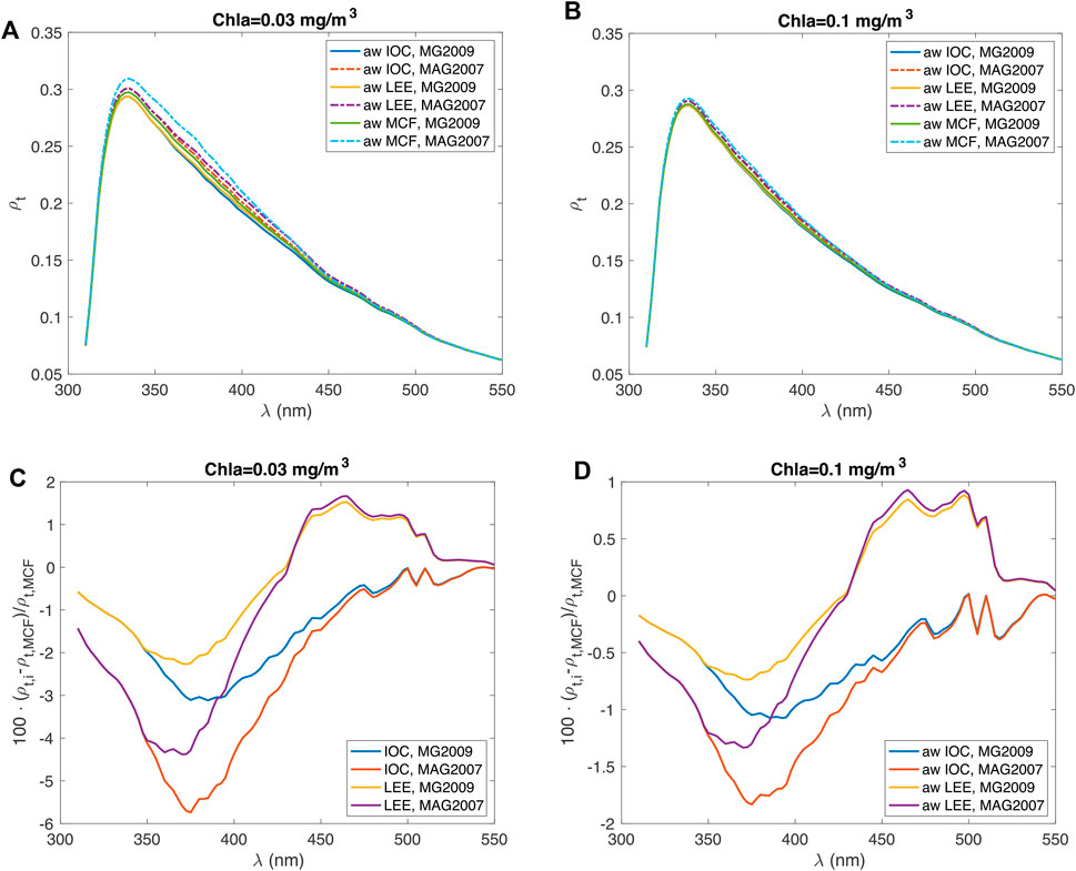
FIGURE 3. (A) the total reflectance at TOA for [Chla] = 0.03 mg/m3. Six curves are shown, corresponding to three sources of water absorption coefficients times two different CDOM absorption parameterization in [Chla]. (B) the same as Figure 3A, except for [Chla] = 0.1 mg/m3. (C) the percentage difference of the TOA reflectance compared to MCF, where the subscript
3.2 Impacts of brown Carbon Aerosols and CDOM to the Polarized Radiance Field at TOA
We used the PACE simulator to simulate polarized reflectance at the TOA for nine cases with different amounts of brown aerosol and CDOM in the coupled atmosphere and ocean system. The wind speed is 5 m/s. The ocean water is assumed to be a mixture of pure seawater, phytoplankton particles, and CDOM. The absorption coefficient of the phytoplankton particles follows the bio-optical model Eq. 4 with [Chla] = 1 mg/m3. The backscattering coefficient at 660 nm
The aerosol optical depth is 0.1 at 550 nm. The aerosol model is assumed to be a bio-modal lognormal distribution, with the fine and coarse modes to be 90 and 10% of the total volume, respectively. The coarse mode is assumed to be sea salt with the effective radius and variance of 2.0194

TABLE 1. The volume fractions of different components for the aerosol models used in the study.
The refractive indices of soot carbon, dust-like, water-soluble, and sea-salt are from Shettle and Fenn (1979). The real refractive index
where
Figure 4 shows the singe scattering albedo of the aerosol models with three different brown carbon volume fractions: 0.02, 0.04, and 0.06 in the fine mode. It shows that the single scattering albedo ranges between 0.915 and 0.965. It is smaller for smaller brown carbon fraction, primarily due to soot carbon which is ½ of brown carbon volume fraction. The separation between the three lines in the UV bands are slightly larger than other spectral region, indicating the influence of brown carbon. In addition, the DoLP signal has different sensitivity to single scattering albedo, which may be used to further differentiate the influence of CDOM and absorbing aerosols.
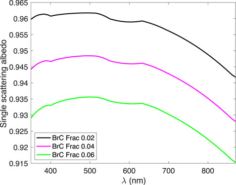
FIGURE 4. The single scattering albedo of the three aerosol models with the brown carbon volume factions of 0.02, 0.04, and 0.06 in the fine mode.
We calculate the percentage difference of the TOA signals for each case in comparison to a reference case, which is
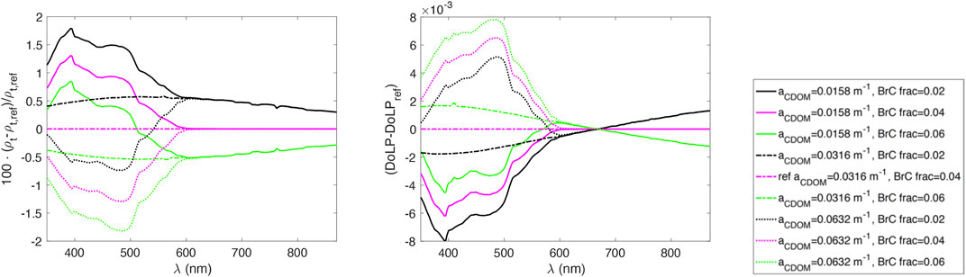
FIGURE 5. Left: the percentage difference of the TOA reflectance with respect to a reference case (ref), which corresponds to
The MAP instruments will measure the polarized radiance at different viewing angles, which can provide extra information on the aerosol and hydrosol microphysics. Figure 6 shows the dependence of DoLP in the principal plane as a function of viewing zenith angle. The principal plane is defined as the plane containing the direct solar ray and local vertical. Positive viewing zenith angles indicate the half plane with an azimuth angle of 0°, which contains the Sun glint, while negative viewing zenith angles are the half plane of an azimuth angle of 180°. Two HARP wavelengths, 441 and 669 nm, are chosen to show the angular dependence. At 441 nm, both the brown carbon fractions and the CDOM absorption coefficients have visible influences on the DoLP at TOA (see Figure 6A, the difference of DoLP with those of a reference case). At 669 nm, the influence due to CDOM absorption diminishes and only brown carbon aerosols would have influences on DoLP (See Figure 6B). The DoLP change at 441 nm is as large as 0.008. It is smaller at 669 nm for which the DoLP change is mostly smaller than 0.00015, which is hard to be differentiated by SPEXone. The angular dependence of DoLP at TOA at different wavelength can be used to differentiate the brown carbon fraction and CDOM absorption if a proper data fitting algorithm is implemented.
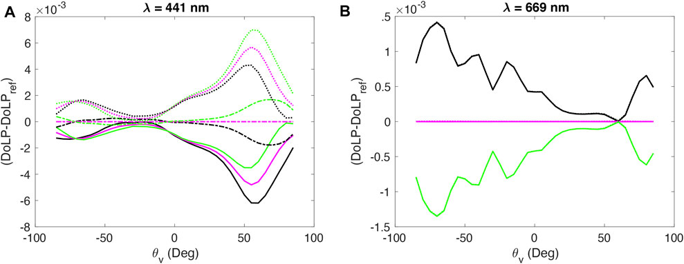
FIGURE 6. (A) DoLP-DoLPref in the principal plane as a function of viewing zenith angle at 441 nm, where ref is corresponds to the case of
4 Discussion
In this paper, we described a PACE simulator that is built upon rigorous radiative transfer models. The monochromatic radiative transfer model is based on the successive order of scattering method for coupled atmosphere and ocean systems. A series of periphery software packages were developed to set up the atmospheric and ocean optical properties as a function of wavelengths. In the atmosphere, the Rayleigh scattering matrix is used for molecular scattering, with the scattering cross-section and depolarization factor calculated based on the atmosphere’s vertical pressure and temperature profiles. The aerosol and cloud properties can be flexibly set. A number of commonly used aerosol models are built in the simulator for the convenience of users, including Shettle and Fenn (1979); Ahmad et al. (2010). Gas absorptions are considered by using a hyperspectral gas absorption cross-section look-up-table calculated with the HITRAN database and a few other suitable sources. In the ocean, a number of different bio-optical models are included to model the scattering and absorption of light by various components, including pure seawater, phytoplankton and their derivative non-algal particles, and CDOM. The model can use chlorophyll-a concentration as a sole parameter to parameterize the ocean water inherent optical properties, which represent the behaviors of open ocean waters. It can provide a number of options where the inherent optical properties of different components do not follow the global average behavior so that we can model the coastal and inland waters. Inelastic scattering of ocean waters, including Raman scattering, fluorescence due to chlorophyll and CDOM can be modeled. All three PACE instruments, OCI, HARP, and SPEXone, are considered. The PACE simulator generates the Stokes parameters (I, Q, U, and V) for a sensor at arbitrary locations in the atmosphere and ocean.
To show an application of the PACE simulator, we present two sensitivity studies in the UV. One is the variation of the TOA radiance field due to the uncertainty of the pure ocean water absorption coefficient. There are some large differences in pure water absorption coefficients in the UV among different sources. We choose the three most credible sources, and their differences are as large as a couple of orders of magnitude. Using a typical setting of the atmosphere and ocean system, we found that the variation of the TOA radiance field is largest for smaller chlorophyll concentrations, which ranges between −6–2% for [Chla] = 0.03 mg/m3 at different wavelengths. For [Chla] = 0.1 mg/m3, the difference reduces to −2–1%. In the second study, we present the influence of different brown carbon fraction and CDOM amount to the polarized radiance field at TOA. We found that the influence of CDOM on the reflectance is for wavelengths smaller than 600 nm, while brown carbon affects the whole spectrum, primarily due to covaried soot aerosols. The polarized signal has a different spectral trend from the reflectance. The angular dependence of DoLP at 441 nm is sensitive to both brown carbon fractions and the CDOM absorption, while the influence of CDOM is minimal at 669 nm. The percentage difference between the different values of the brown carbon fraction (0.02, 0.04, and 0.06) is of the order of 1–2%, which can be detected by the OCI instrument, whose goal is to achieve 0.5% calibration accuracy. The DoLP variation is around 0.008, which can also be detected by SPEXone whose DoLP accuracy requirement is 0.003. These properties can be used to design remote sensing algorithms which retrieve the brown carbon and CDOM abundance.
In summary, our PACE simulator can be used in a wide range of applications, including sensitivity studies of different atmosphere and ocean components, the generation of synthetic data for testing remote sensing algorithms, and building look-up tables for atmospheric correction of ocean color remote sensing.
Data Availability Statement
The original contributions presented in the study are included in the article/Supplementary Material, further inquiries can be directed to the corresponding author.
Author Contributions
P-WZ and YH developed the original radiative transfer concept. P-WZ implemented the simulation algorithm and generated the sensitivity study. BF and MG advised on the PACE instrument characteristics. PJW and AI provided bio-optical model used in the simulator. PJW advised on the ocean water absorption sensitivity study. YH provided advice on the data analysis. JC suggested on brown carbon microphysical properties. All authors contributed to the editing of the manuscript.
Funding
This research is partially supported by NASA Grants 80NSSC20M0227 and 80NSSC18K0345.
Conflict of Interest
Author MG was employed by Science Systems and Applications Inc.
The remaining authors declare that the research was conducted in the absence of any commercial or financial relationships that could be construed as a potential conflict of interest.
Publisher’s Note
All claims expressed in this article are solely those of the authors and do not necessarily represent those of their affiliated organizations, or those of the publisher, the editors and the reviewers. Any product that may be evaluated in this article, or claim that may be made by its manufacturer, is not guaranteed or endorsed by the publisher.
References
Ahmad, Z., Franz, B. A., McClain, C. R., Kwiatkowska, E. J., Werdell, J., Shettle, E. P., et al. (2010). New Aerosol Models for the Retrieval of Aerosol Optical Thickness and Normalized Water-Leaving Radiances from the SeaWiFS and MODIS Sensors over Coastal Regions and Open Oceans. Appl. Opt. 49, 5545–5560. doi:10.1364/ao.49.005545
Bi, L., and Yang, P. (2014). Accurate Simulation of the Optical Properties of Atmospheric Ice Crystals with the Invariant Imbedding T-Matrix Method. J. Quantitative Spectrosc. Radiative Transfer 138, 17–35. doi:10.1016/j.jqsrt.2014.01.013
Braslau, N., and Dave, J. V. (1973). Effect of Aerosols on the Transfer of Solar Energy through Realistic Model Atmospheres. Part I: Non-absorbing Aerosols. J. Appl. Meteorol. 12, 601–615. doi:10.1175/1520-0450(1973)012<0601:eoaott>2.0.co;2
Bricaud, A., Babin, M., Claustre, H., Ras, J., and Tièche, F. (2010). Light Absorption Properties and Absorption Budget of Southeast Pacific Waters. J. Geophys. Res. 115, C08009. doi:10.1029/2009jc005517
Bricaud, A., Morel, A., Babin, M., Allali, K., and Claustre, H. (1998). Variations of Light Absorption by Suspended Particles with Chlorophyllaconcentration in Oceanic (Case 1) Waters: Analysis and Implications for Bio-Optical Models. J. Geophys. Res. 103, 31033–31044. doi:10.1029/98jc02712
Buehler, S. A., Mendrok, J., Eriksson, P., Perrin, A., Larsson, R., and Lemke, O. (2018). ARTS, the Atmospheric Radiative Transfer Simulator - Version 2.2, the Planetary Toolbox Edition. Geosci. Model. Dev. 11 (4), 1537–1556. doi:10.5194/gmd-11-1537-2018
Burrows, J. P., Dehn, A., Deters, B., Himmelmann, S., Richter, A., Voigt, S., et al. (1998). Atmospheric Remote-Sensing Reference Data from Gome: Part 1. Temperature-dependent Absorption Cross-Sections of No2 in the 231-794 Nm Range. J. Quantitative Spectrosc. Radiative Transfer 60, 1025–1031. doi:10.1016/s0022-4073(97)00197-0
Chowdhary, J., Zhai, P.-W., Xu, F., Frouin, R., and Ramon, D. (2020). Testbed Results for Scalar and Vector Radiative Transfer Computations of Light in Atmosphere-Ocean Systems. J. Quantitative Spectrosc. Radiative Transfer 242, 106717. doi:10.1016/j.jqsrt.2019.106717
Cox, C., and Munk, W. (1954). Measurement of the Roughness of the Sea Surface from Photographs of the Sun's Glitter. J. Opt. Soc. Am. 44, 838–850. doi:10.1364/josa.44.000838
Duan, M., Min, Q., and Li, J. (2005). A Fast Radiative Transfer Model for Simulating High-Resolution Absorption Bands. J. Geophys. Res. 110, D15201. doi:10.1029/2004JD005590
Gordon, I. E., Rothman, L. S., and Hill, C. (2017). The HITRAN2016 Molecular Spectroscopic Database. J. Quant. Spectrosc. Radiat. Transf. 203, 3–69. doi:10.15278/isms.2017.tj09
Gregg, W. W., and Rousseaux, C. S. (2017). Simulating PACE Global Ocean Radiances. Front. Mar. Sci. 4, 1–19. doi:10.3389/fmars.2017.00060
Hasekamp, O. P., Fu, G., Rusli, S. P., Wu, L., Di Noia, A., Brugh, J. A. D., et al. (2019). Aerosol Measurements by SPEXone on the NASA PACE mission: Expected Retrieval Capabilities. J. Quantitative Spectrosc. Radiative Transfer 227, 170–184. doi:10.1016/j.jqsrt.2019.02.006
Hovenier, J. W., Van Der Mee, C., and Domke, H. (2004). Transfer of Polarized Light in Planetary Atmospheres. Basic concepts Pract. Methods 318. doi:10.1007/978-1-4020-2856-4
Hu, Y.-X., Wielicki, B., Lin, B., Gibson, G., Tsay, S.-C., Stamnes, K., et al. (2000). δ-Fit: A Fast and Accurate Treatment of Particle Scattering Phase Functions with Weighted Singular-Value Decomposition Least-Squares Fitting. J. Quantitative Spectrosc. Radiative Transfer 65, 681–690. doi:10.1016/s0022-4073(99)00147-8
Ibrahim, A., Gilerson, A., Chowdhary, J., and Ahmed, S. (2016). Retrieval of Macro- and Micro-physical Properties of Oceanic Hydrosols from Polarimetric Observations. Remote Sensing Environ. 186, 548–566. doi:10.1016/j.rse.2016.09.004
Lee, Z., Wei, J., Voss, K., Lewis, M., Bricaud, A., and Huot, Y. (2015). Hyperspectral Absorption Coefficient of "pure" Seawater in the Range of 350-550 Nm Inverted from Remote Sensing Reflectance. Appl. Opt. 54, 546–558. doi:10.1364/ao.54.000546
Lin, Z., Chen, N., Fan, Y., Li, W., Stamnes, K., and Stamnes, S. (2018). New Treatment of Strongly Anisotropic Scattering Phase Functions: The Delta-M+ Method. J. Atmos. Sci. 75 (1), 327–336. doi:10.1175/jas-d-17-0233.1
Mason, J. D., Cone, M. T., and Fry, E. S. (2016). Ultraviolet (250-550 Nm) Absorption Spectrum of Pure Water. Appl. Opt. 55, 7163–7172. doi:10.1364/ao.55.007163
McBride, B. A., Martins, J. V., Barbosa, H. M. J., Birmingham, W., and Remer, L. A. (2020). Spatial Distribution of Cloud Droplet Size Properties from Airborne Hyper-Angular Rainbow Polarimeter (AirHARP) Measurements. Atmos. Meas. Tech. 13, 1777–1796. doi:10.5194/amt-13-1777-2020
Mishchenko, M. I., Travis, L. D., and Lacis, A. A. (2002). Scattering, Absorption, and Emission of Light by Small Particles. Cambridge: Cambridge University Press.
Mobley, C. D., Gentili, B., Gordon, H. R., Jin, Z., Kattawar, G. W., Morel, A., et al. (1993). Comparison of Numerical Models for Computing Underwater Light fields. Appl. Opt. 32, 7484–7504. doi:10.1364/ao.32.007484
Mobley, C. D. (1994). Light and Water: Radiative Transfer in Natural Waters. San Diego, CA: Academic Press.
Mok, J., Krotkov, N. A., Arola, A., Torres, O., Jethva, H., Andrade, M., et al. (2016). Impacts of Brown Carbon from Biomass Burning on Surface UV and Ozone Photochemistry in the Amazon Basin. Sci. Rep. 6, 36940. doi:10.1038/srep36940
Morel, A., Claustre, H., Antoine, D., and Gentili, B. (2007). Natural Variability of Bio-Optical Properties in Case 1 Waters: Attenuation and Reflectance within the Visible and Near-UV Spectral Domains, as Observed in South Pacific and Mediterranean Waters. Biogeosciences 4, 913–925. doi:10.5194/bg-4-913-2007
Morel, A., and Gentili, B. (2009). A Simple Band Ratio Technique to Quantify the Colored Dissolved and Detrital Organic Material from Ocean Color Remotely Sensed Data. Remote Sensing Environ. 113, 998–1011. doi:10.1016/j.rse.2009.01.008
Morel, A., and Maritorena, S. (2001). Bio-optical Properties of Oceanic Waters: A Reappraisal. J. Geophys. Res. 106 (C4), 7163–7180. doi:10.1029/2000JC000319
Morrison, R. J., and Goodwin, D. S. (2010). Phytoplankton Photocompensation from Space Based Fluorescence Measurements. Geophys. Res. Lett. 37. doi:10.1029/2009gl041799
Pope, R. M., and Fry, E. S. (1997). Absorption Spectrum (380-700 Nm) of Pure Water II Integrating Cavity Measurements. Appl. Opt. 36, 8710–8723. doi:10.1364/ao.36.008710
Schuster, G. L., Dubovik, O., and Arola, A. (2016). Remote Sensing of Soot Carbon - Part 1: Distinguishing Different Absorbing Aerosol Species. Atmos. Chem. Phys. 16, 1565–1585. doi:10.5194/acp-16-1565-2016
Serdyuchenko, A., Gorshelev, V., Weber, M., Chehade, W., and Burrows, J. P. (2014). High Spectral Resolution Ozone Absorption Cross-Sections - Part 2: Temperature Dependence. Atmos. Meas. Tech. 7, 625–636. doi:10.5194/amt-7-625-2014
Shettle, E. P., and Fenn, R. W. (1979). Models for the Aerosols of the Lower Atmosphere and the Eects of Humidity Variations on Their Optical Properties, AFGL-TR-79-0214 U.S. Mass: Air Force Geophysics Laboratory, Hanscom Air Force Base.
Shi, C., Hashimoto, M., Shiomi, K., and Nakajima, T. (2021). Development of an Algorithm to Retrieve Aerosol Optical Properties over Water Using an Artificial Neural Network Radiative Transfer Scheme: First Result from GOSAT-2/CAI-2. IEEE Trans. Geosci. Remote Sensing 59, 9861–9872. doi:10.1109/TGRS.2020.3038892
Sumlin, B. J., Heinson, Y. W., Shetty, N., Pandey, A., Pattison, R. S., Baker, S., et al. (2018). UV-Vis-IR Spectral Complex Refractive Indices and Optical Properties of Brown Carbon Aerosol from Biomass Burning. J. Quantitative Spectrosc. Radiative Transfer 206, 392–398. doi:10.1016/j.jqsrt.2017.12.009
Sun, W., Hu, Y., Weimer, C., Ayers, K., Baize, R. R., and Lee, T. (2017). A FDTD Solution of Scattering of Laser Beam with Orbital Angular Momentum by Dielectric Particles: Far-Field Characteristics. J. Quantitative Spectrosc. Radiative Transfer 188, 200–213. doi:10.1016/j.jqsrt.2016.02.006
Tomasi, C., Vitale, V., Petkov, B., Lupi, A., and Cacciari, A. (2005). Improved Algorithm for Calculations of Rayleigh-Scattering Optical Depth in Standard Atmospheres. Appl. Opt. 44, 3320–3341. doi:10.1364/ao.44.003320
Twardowski, M., Röttgers, R., and Stramski, D. (2018). “Chapter 1: The Absorption Coefficient, an Overview, in Inherent Optical Property Measurements and Protocols: Absorption Coefficient,” in IOCCG Ocean Optics and Biogeochemistry Protocols for Satellite Ocean Colour Sensor Validation. Editors A. R. Neeley, and A. Mannino (Dartmouth, NS, Canada: IOCCG), 1.0.
Twardowski, M. S., Boss, E., Sullivan, J. M., and Donaghay, P. L. (2004). Modeling the Spectral Shape of Absorption by Chromophoric Dissolved Organic Matter. Mar. Chem. 89, 69–88. doi:10.1016/j.marchem.2004.02.008
U.S. (19761976). Standard Atmosphere. Washington, D.C.: U.S. Government Printing Office. https://ccmc.gsfc.nasa.gov/modelweb/atmos/us_standard.html.
Voss, K. J. (1992). A Spectral Model of the Beam Attenuation Coefficient in the Ocean and Coastal Areas. Limnol. Oceanogr. 37, 501–509. doi:10.4319/lo.1992.37.3.0501
Voss, K. J., and Fry, E. S. (1984). Measurement of the Mueller Matrix for Ocean Water. Appl. Opt. 23, 4427–4439. doi:10.1364/ao.23.004427
Werdell, P. J., Behrenfeld, M. J., Bontempi, P. S., Boss, E., Cairns, B., Davis, G. T., et al. (2019). The Plankton, Aerosol, Cloud, Ocean Ecosystem Mission: Status, Science, Advances. Advances, Bull. Am. Meteorol. Soc. 100 (9), 1775–1794. doi:10.1175/BAMS-D-18-0056.1
Whitmire, A. L., Boss, E., Cowles, T. J., and Pegau, W. S. (2007). Spectral Variability of the Particulate Backscattering Ratio. Opt. Express 15, 7019–7031. doi:10.1364/oe.15.007019
Wiscombe, W. J. (1977). The Delta-MMethod: Rapid yet Accurate Radiative Flux Calculations for Strongly Asymmetric Phase Functions. J. Atmos. Sci. 34, 1408–1422. doi:10.1175/1520-0469(1977)034<1408:tdmrya>2.0.co;2
Yang, P., and Liou, K. N. (1996). Finite-difference Time Domain Method for Light Scattering by Small Ice Crystals in Three-Dimensional Space. J. Opt. Soc. Am. A. 13, 2072–2085. doi:10.1364/josaa.13.002072
Yurkin, M. A., and Hoekstra, A. G. (2011). The Discrete-Dipole-Approximation Code ADDA: Capabilities and Known Limitations. J. Quantitative Spectrosc. Radiative Transfer 112, 2234–2247. doi:10.1016/j.jqsrt.2011.01.031
IOCCG (2006). “Remote Sensing of Inherent Optical Properties: Fundamentals, Tests of Algorithms, and Applications,” in Reports of the International Ocean-Colour Coordinating Group, No. 5. Editor Z. P. Lee (Dartmouth, Canada: IOCCG).
Zhai, P.-W., Boss, E., Franz, B., Werdell, P., and Hu, Y. (2018). Radiative Transfer Modeling of Phytoplankton Fluorescence Quenching Processes. Remote Sensing 10, 1309. doi:10.3390/rs10081309
Zhai, P.-W., Hu, Y., Chowdhary, J., Trepte, C. R., Lucker, P. L., and Josset, D. B. (2010). A Vector Radiative Transfer Model for Coupled Atmosphere and Ocean Systems with a Rough Interface. J. Quantitative Spectrosc. Radiative Transfer 111, 1025–1040. doi:10.1016/j.jqsrt.2009.12.005
Zhai, P.-W., Hu, Y., Josset, D. B., Trepte, C. R., Lucker, P. L., and Lin, B. (2013). Advanced Angular Interpolation in the Vector Radiative Transfer for Coupled Atmosphere and Ocean Systems. J. Quantitative Spectrosc. Radiative Transfer 115, 19–27. doi:10.1016/j.jqsrt.2012.09.018
Zhai, P.-W., Hu, Y., Josset, D. B., Trepte, C. R., Lucker, P. L., and Lin, B. (2012). “Exact First Order Scattering Correction for Vector Radiative Transfer in Coupled Atmosphere and Ocean Systems,” in Polarization: Measurement, Analysis, and Remote Sensing X, 8364. doi:10.1117/12.920767
Zhai, P.-W., Hu, Y., Trepte, C. R., and Lucker, P. L. (2009). A Vector Radiative Transfer Model for Coupled Atmosphere and Ocean Systems Based on Successive Order of Scattering Method. Opt. Express 17, 2057–2079. doi:10.1364/oe.17.002057
Zhai, P.-W., Hu, Y., Winker, D. M., Franz, B. A., and Boss, E. (2015). Contribution of Raman Scattering to Polarized Radiation Field in Ocean Waters. Opt. Express 23 (18), 23582–23596. doi:10.1364/oe.23.023582
Zhai, P.-W., Hu, Y., Winker, D. M., Franz, B. A., Werdell, J., and Boss, E. (2017b). Vector Radiative Transfer Model for Coupled Atmosphere and Ocean Systems Including Inelastic Sources in Ocean Waters. Opt. Express 25, A223–A239. doi:10.1364/oe.25.00a223
Zhai, P.-W., Knobelspiesse, K., Ibrahim, A., Franz, B. A., Hu, Y., Gao, M., et al. (2017a). Water-leaving Contribution to Polarized Radiation Field over Ocean. Opt. Express 25, A689–A708. doi:10.1364/oe.25.00a689
Keywords: PACE, radiative transfer, ocean color, ultraviolet, CDOM, Brown carbon aerosols
Citation: Zhai P-W, Gao M, Franz BA, Werdell PJ, Ibrahim A, Hu Y and Chowdhary J (2022) A Radiative Transfer Simulator for PACE: Theory and Applications. Front. Remote Sens. 3:840188. doi: 10.3389/frsen.2022.840188
Received: 20 December 2021; Accepted: 17 January 2022;
Published: 14 February 2022.
Edited by:
Feng Xu, University of Oklahoma, United StatesReviewed by:
Chong Shi, Aerospace Information Research Institute (CAS), ChinaBo-Cai Gao, United States Naval Research Laboratory, United States
Copyright © 2022 Zhai, Gao, Franz, Werdell, Ibrahim, Hu and Chowdhary. This is an open-access article distributed under the terms of the Creative Commons Attribution License (CC BY). The use, distribution or reproduction in other forums is permitted, provided the original author(s) and the copyright owner(s) are credited and that the original publication in this journal is cited, in accordance with accepted academic practice. No use, distribution or reproduction is permitted which does not comply with these terms.
*Correspondence: Peng-Wang Zhai, cHd6aGFpQHVtYmMuZWR1