Evaluating the effective resolution of enhanced resolution SMAP brightness temperature image products

The MEaSUREs Calibrated Enhanced-Resolution Passive Microwave Daily Equal-Area Scalable Earth Grid 2.0 Brightness Temperature (CETB) Earth System Data Record (ESDR) includes conventional- and enhanced-resolution radiometer brightness temperature (T_B) images on standard, compatible grids from calibrated satellite radiometer measurements collected over a multi-decade period. Recently, the CETB team processed the first 4 years of enhanced resolution Soil Moisture Active Passive (SMAP) L-band (1.41 GHz) radiometer T_B images. The CETB processing employs the radiometer form of the Scatterometer Image Reconstruction (rSIR) algorithm to create enhanced resolution images, which are posted on fine resolution grids. In this paper, we evaluate the effective resolution of the SMAP T_B image products using coastline and island crossings. We similarly evaluate the effective resolution of the SMAP L1C_TB_E enhanced resolution product that is based on Backus-Gilbert processing. We present a comparison of the spatial resolution of the rSIR and L1C_TB_E enhanced resolution products with conventionally-processed (gridded) SMAP data. We find that the effective resolution of daily CETB rSIR SMAP T_B images is slightly finer than that of L1C_TB_E and about 30% finer than conventionally processed data.

1 Introduction

The NASA MEaSUREs Calibrated Enhanced-Resolution Passive Microwave Daily Equal-Area Scalable Earth Grid 2.0 Brightness Temperature (CETB) Earth System Data Record (ESDR) is a single, consistently processed, multi-sensor ESDR of Earth-gridded microwave brightness temperature (T_B) images that span from 1978 to the present (Brodzik et al., 2018; Brodzik and Long, 2016). It is based on new fundamental climate data records (FCDRs) for passive microwave observations from a wide array of sensors (Berg et al., 2018). The CETB dataset includes both conventional- and enhanced-resolution T_B images on standard map projections and is designed to serve the land surface and polar snow/ice research communities in studies of climate and climate change (Long and Brodzik, 2016). Recently, T_B image products from L-band Soil Moisture Active Passive (SMAP) radiometer (Entekhabi et al., 2010; Piepmeier et al., 2017) data were added to the CETB dataset (Long et al., 2019; Brodzik et al., 2021).

Conventional-resolution CETB T_B images are created using standard drop-in-the-bucket (DIB) techniques, also known as gridding (GRD). To create finer resolution images, reconstruction techniques are employed (Long and Brodzik, 2016). The images are produced on compatible map projections and grid spacings (Brodzik and Long, 2016; Brodzik et al., 2021). Previous papers have used simulation to compare the resolution enhancement capabilities of the radiometer form of the Scatterometer Image Reconstruction (rSIR) algorithm and the Backus-Gilbert (BG) approach (Backus and Gilbert, 1967; Backus and Gilbert, 1968), where it was found that rSIR provides improved performance compared to BG with significantly less computation (Long and Brodzik, 2016; Long et al., 2019).

The CETB products combine multiple orbit passes, which increases the sampling density, into a twice-daily product. For rSIR, the increased sampling density permits the algorithm to extract finer spatial information. In contrast, the enhanced resolution SMAP L1C_TB_E product (Chaubell, 2016; Chaubell et al., 2016; Chaubell et al., 2018) is created from individual 1/2 orbits using a version of the BG interpolation approach (Backus and Gilbert, 1967, 1968; Poe, 1990). To reiterate, one important difference between the two products is multiple passes are combined in the rSIR processing to create hemisphere images, whereas only a single pass is used in BG processing of the swath-based L1C_TB_E product. Both rSIR and L1C_TB_E exhibit finer spatial resolution than conventional GRD processing as defined by the 3 dB width of the pixel spatial response function (PSRF).

In this paper, actual SMAP data are used to measure and compare the effective spatial resolution of the rSIR and L1C_TB_E enhanced resolution products. The results are compared to the effective resolution of conventional gridded processing. The paper is organized as follows: after some brief background in Sec. II, a discussion of the measurement and pixel spatial measurement response functions is provided in Sec. III. Section IV presents estimates of the response functions. A discussion of posting versus effective resolution is given in Sec. V, followed by a summary conclusion in Sec. VI.

2 Background

The SMAP radiometer operates at L-band (1.41 GHz) with a 24 MHz bandwidth, and collects measurements of the horizontal (H), vertical (V), and 3rd and 4th Stokes parameter polarizations with a total radiometric uncertainty of 1.3 K (Piepmeier et al., 2017; Piepmeier et al., 2014). The SMAP spacecraft was launched in January 2015 and flies in a 98.1° inclination sun-synchronous polar orbit at 685 km altitude. SMAP collects overlapping T_B measurements over a wide swath using an antenna rotating at 14.6 rpm. The nominal 3-dB elliptical footprint is 39 km by 47 km (Piepmeier et al., 2014; Piepmeier et al., 2017; Long et al., 2019).

2.1 Enhanced resolution SMAP T_B products

CETB products are created by mapping individual T_B measurements onto an Earth-based grid using standard Equal-Area Scalable Earth Grid 2.0 (EASE2) map projections (Brodzik et al., 2012; Brodzik et al., 2014). In the GRD conventional-resolution gridded CETB product, the center of each measurement location is mapped to a map-projected grid cell or pixel. All measurements within the specified time period whose centers fall within the bounds of a particular grid cell are averaged together (Brodzik and Long, 2016). The unweighted average becomes the reported pixel T_B value for that grid cell. Since measurement footprints can extend outside of the pixel, the effective resolution of GRD images is coarser than the pixel size. We call the spacing of the pixel centers the posting or the posting resolution, see Figure 1.

FIGURE 1

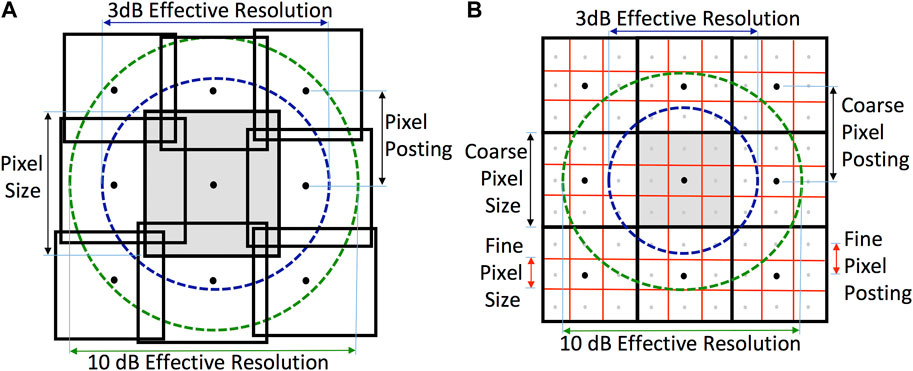
FIGURE 1. Pixel size versus posting illustrations. (A) Diagram showing irregularly sized and overlapping pixels posted on a uniform grid. Due to the processing used to compute the pixel value, the 3 dB contour of the pixel spatial response function (PSRF) is larger than the pixel area. A 10 dB contour of PSRF is shown for comparison. (B) Diagram of uniform grids showing both fine and coarse pixels. The effective resolution of the PSRF of both coarse and fine pixels is the same, with the fine pixels posted at finer spacing (resolution).

Finer spatial resolution CETB products are generated using reconstruction with the rSIR algorithm (Long and Daum, 1998; Long and Brodzik, 2016). The iterative rSIR algorithm employs regularization to tradeoff noise and resolution by limiting the number of iterations and thereby producing partial reconstruction (Long et al., 2019). The rSIR products are posted on fine resolution grids with an effective resolution that is coarser than the posting resolution; i.e., they are oversampled (Long and Brodzik, 2016). For SMAP the CETB generates global cylindrical equal-area T_B images using GRD at both 36 km and 25 km postings and rSIR-enhanced T_B images on nested EASE2-grids at 3, 3.125, and 8 km postings (Brodzik and Long, 2016). We note that the finest spatial frequency that can be represented in a sampled image is twice the posting resolution, though the effective resolution can be coarser than this (McLinden et al., 2015). The different postings in the CETB enable users to readily analyze data from multiple sensors (Brodzik and Long, 2016).

The SMAP L1C_TB_E product is also produced on standard EASE2 map projections, but only at a single posting resolution of 9 km (Chaubell, 2016; Chaubell et al., 2016). This product uses BG-based optimal interpolation to estimate T_B over the swath, interpolated to the grid pixels based on the instrument T_B measurements (Poe, 1990) on a per-orbit (single-pass) basis. The key differences between the CETB and L1C_TB_E products are how multiple passes are treated. The L1C_TB_E product is generated on a per pass basis with one image product per pass, while the CETB product combines multiple passes into twice-daily images, i.e., two images per day. The CETB product enables somewhat better effective spatial resolution with limited impact on the temporal resolution and few individual files.

2.2 Pixel and measurement response functions

The SMAP radiometer collects measurements over an irregular grid. As described below, each measurement has a unique spatial measurement response function (MRF) that describes the contribution of each point on the surface to the measured value. The measurements, possibly from multiple orbit passes, are processed into a uniform pixel grid. The value report for each grid element or pixel is a weighted sum of multiple measurements. The pixel spatial response function (PSRF) describes the contribution of each point on the surface to the reported pixel value, i.e., how much the brightness temperature at a particular spatial location contributes to the reported brightness temperature of the pixel. In effect, the PSRF is the impulse response of the measurement system for a particular pixel. The PSRF includes the image formation process as well as the effects of the sampling and the measurement MRFs that are combined into the reported pixel value. In contrast, the MRF is just the spatial response of a single measurement. Analysis of the PSRF defines the effective resolution of the image formation.

We note that in general, the extent of spatial response function of a pixel in a remote sensing image can be larger than its spacing (the posting resolution) so that the effective extent of the pixels overlap, as illustrated in Figure 1, i.e., the pixel size is greater than the posting resolution. This means that the effective resolution of the image is coarser than the posting resolution (Long and Brodzik, 2016). When the posting resolution is finer than the effective resolution, the signal is sometimes termed oversampled as illustrated in Figure 1. While in principle in such cases the image can be resampled to a coarser posting resolution with limited loss of information, deliberate oversampling provides flexibility in resampling the data and is the approach taken by CETB when it reports images on map-standard pixel sizes (posting resolutions).

2.3 Radiometer spatial measurement response function

This section provides a brief summary of the derivation of the MRF of the SMAP radiometer sensor and the algorithms used for T_B image construction from the measurements. The effective spatial resolution of the image products is determined by the MRF and by the image formation algorithm used. The MRF is determined by the antenna gain pattern, the scan geometry (notably the antenna scan angle), and the integration period. We note that for T_B image reconstruction, the MRF is treated as non-zero only in the direction of the surface.

The MRF for a general microwave radiometer is derived in (Long and Brodzik, 2016; Long et al., 2019). Microwave radiometers measure the thermal emission from natural surfaces (Ulaby and Long, 2014). In a typical satellite radiometer, an antenna is scanned over the scene of interest and the output power from the carefully calibrated receiver is measured as a function of scan position. The reported signal is a temporal average of the filtered received signal power. The observed power is related to receiver gain and noise figure, antenna loss, physical temperature of the antenna, antenna pattern, and scene brightness temperature (Ulaby and Long, 2014).

Because the antenna is rotating and moving during the integration period, the effective antenna gain pattern G_s is a smeared version of the instantaneous antenna pattern. The observed brightness temperature measurement z can be expressed as

$z=\int \int \mathrm{M}\mathrm{R}\mathrm{F}\left(x,y\right)T_B\left(x,y\right)dxdy(1)$

where MRF(x, y) is the measurement response function expressed in surface coordinates x, y (Long and Brodzik, 2016). It is the normalized effective antenna gain pattern,

$\mathrm{M}\mathrm{R}\mathrm{F}\left(x,y\right)=G_b^{-1}{G}_s\left(x,y\right)(2)$

where G_b is the integrated gain,

$G_b=\int \int G_s\left(x,y\right)dxdy.(3)$

In effect, the MRF describes to what extent the emissions from a particular location on the surface contribute to the observed T_B value. A typical SMAP MRF has an elliptical, nearly Gaussian shape that is centered at the measurement location (Long et al., 2019). Due to the varying observation geometry (orbit, oblate Earth, and azimuth scanning), the MRF varies between measurements.

2.4 Sampling considerations

The SMAP radiometer is conically scanning. Integrated T_B measurements are collected at fixed 17 ms intervals (Piepmeier et al., 2014), which yields an along-scan spacing of approximately 11 km. Due to the motion of the spacecraft between antenna rotations, the nominal along-track spacing is approximately 28 km. This yields a surface sampling density of approximately 11 km × 28 km, which according to the Nyquist criterion can unambiguously support wavenumbers (spatial frequencies) up to 1/22 km⁻¹ × 1/56 km⁻¹ when including data from a single pass. However, the MRF includes information from higher wavenumbers than this. This information can alias into lower wavenumbers (Skou, 1988; McLinden et al., 2015). Combining multiple passes increases the sampling density, which can support higher wavenumbers and avoid aliasing. The tradeoff of combining multiple passes is reduced temporal resolution.

2.5 Image formation

The image formation process estimates the surface brightness temperature map T_B(x, y) from the calibrated measurements z. This can be done on a swath-based grid (i.e., in swath coordinates) or on an Earth-based map projection grid (Brodzik and Long, 2016), as done in CETB and L1C_TB_E image production. This paper considers only an Earth-based map projection grid.

The simplest image formation algorithm is DIB (GRD), where the measurements whose centers fall within a map grid element (pixel) are averaged into that pixel. The effective resolution of GRD imaging is coarser than the effective resolution of a measurement since individual measurements included in the pixel value extend outside of the pixel area and their centers are spread out within the pixel; thus, the effective resolution is coarser than the posting resolution. Various inverse distance-weighting averaging techniques have been used to improve on DIB. The weighting acts like a signal processing window (McLinden et al., 2015).

Reconstruction techniques can yield finer effective resolution so long as the spatial sampling requirements are met (Skou, 1988; Early and Long, 2001). In the reconstruction algorithms, the MRF for each measurement is used in estimating the surface T_B on a fine-scale grid (Long and Brodzik, 2016; Long et al., 2019). The rSIR algorithm has proven to be effective in generating high resolution T_B images for SMAP (Long et al., 2019). The rSIR estimate approximates a maximum-entropy solution to an underdetermined equation and least-squares solution to an overdetermined system. rSIR provides results superior to the BG method with significantly less computation (Long and Brodzik, 2016). rSIR uses truncated iteration to enable a tradeoff between signal reconstruction accuracy and noise enhancement. Since reconstruction yields finer effective resolution, the image products are called ‘enhanced resolution.’ The enhancement at a particular location depends on the local input measurement density and the MRF, which can vary with each measurement. As discussed in (Long et al., 2019), in order to meet Nyquist requirements for the rSIR signal processing, the posting resolution in the images must be finer than the effective resolution by at least a factor of two.

An alternate approach to reconstruction is optimal interpolation. The BG optimal interpolation approach was introduced to radiometer measurements by Poe (1990), and used for the L1C_TB_E product (Chaubell, 2016; Chaubell et al., 2016). This approach estimates the pixel value on a fine grid as the weighted sum of nearby measurements (Long and Daum, 1998) where the weights are determined from the MRF. Solving for the weights involves a matrix inversion that includes a subjectively selected weighting between the antenna pattern contribution and the noise correlation function. The result has finer resolution than GRD processing, but somewhat less than rSIR (Long and Daum, 1998), which the results in Sec. IV confirm.

3 Pixel spatial response function

As noted previously, the MRF describes the spatial characteristics of an individual measurement, i.e., how much the brightness temperature at each spatial location contributes to the measurement, while PSRF describes the spatial characteristics of reported pixel values, i.e., how much the brightness temperature at a particular spatial location contributes to the reported brightness temperature of the pixel value. Analysis of the PSRF defines the effective resolution of the image formation.

The PSRF can be computed using the MRFs of the individual measurements combined into a particular pixel. For linear image formation algorithms such as GRD, the PSRF is the linear sum of the MRFs of the measurements included in the pixel (Long and Brodzik, 2016). Note, however, that the PSRF varies from pixel to pixel due to the differences in location of the measurement within the pixel area and variations of the measurement MRFs (Long et al., 2019). We further note that the variation in the MRFs between measurements precludes the use of classic deconvolution algorithms, which require a fixed response function. Typically, the PSRF is normalized to a peak value of 1.

While the pixel value in BG is linearly related to the measurements in BG optimal interpolation, the weights used in the interpolation vary non-linearly with pixel and measurement location. This complicates estimation of the PSRF for algorithms that employ BG. Similarly, the non-linearity in the rSIR algorithm complicates computing the PSRF. Prior studies have relied on simulation to compute the PSRF using simulated impulse function (Long and Brodzik, 2016; Long et al., 2019). In this paper we use actual SMAP data to estimate the PSRF for both L1C_TB_E and rSIR products.

Given the PSRF, the effective resolution of an image corresponds to the area of the PSRF greater than a particular threshold, typically −3 dB (Ulaby and Long, 2014; Long et al., 2019). We often express the resolution in terms of the square root of the area, which we call the “linear resolution” in this paper. For example, the ideal PSRF for a rectilinear image is a two-dimensional “rect” or “box-car” function that has a value of 1 over the pixel area and 0 elsewhere, see Figure 2. The ideal posting resolution of an image consisting of 36 km square pixels is 1296 km², which corresponds to a linear resolution of 36 km.

FIGURE 2

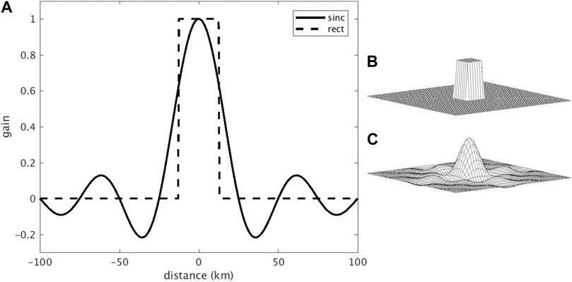
FIGURE 2. (A) A one-dimensional sinc function with a 36 km 3-dB mainlobe width compared to a rect function of the same width. Illustrations of two-dimensional (B) rect and (C) sinc functions.

Since only a finite number of discrete measurements are possible, we must unavoidably assume that the signal and the PSRF are bandlimited such that they are consistent with the sample spacing (Long and Franz, 2016). A bandlimited version of this ideal boxcar PSRF is a two-dimensional sinc function, as seen in Figure 2. For ideal 36 km sampling, this bandlimited PSRF is the best achievable PSRF that is consistent with the sampling. By the Nyquist criterion, signals with frequency higher than 1/2 the sampling rate (posting) cannot be represented without aliasing.

A common way to quantify the effective resolution is the value of the area corresponding to when the PSRF is greater than 1/2, known as the 3 dB PSRF size (Ulaby and Long, 2014). The effective resolution (the 3 dB PSRF size) is larger than the pixel size, and thus is larger than the posting resolution. Note that if we choose a smaller PSRF size threshold, e.g., −10 dB instead of −3 dB, the area is even larger. When the posting resolution is finer than the effective resolution (i.e., the image is oversampled as illustrated in Figure 1) the image can, in principle, be resampled to a coarser posting resolution with limited loss of information (Meier and Stewart, 2020). However, deliberate oversampling provides flexibility in resampling the data, and is the approach taken by CETB when it reports images on map-standard pixel grids with fine posting resolution. The finer posting preserves as much information as possible.

One way to determine the effective resolution is based on first estimating the step response of the imaging process. By assuming the PSRF is symmetric, the PSRF can be derived from the observed step response, greatly simplifying the process of estimating the effective resolution. Recall that the step response is mathematically the convolution of the PSRF with a step function. The PSRF can thus be computed from the step response by deconvolution with a step function. In this case the deconvolution product represents a slice of the PSRF. The effective linear resolution is the width of the PSRF above the −3 dB threshold.

4 Resolution estimation of actual data

In this section, we evaluate the effective linear resolution of SMAP image data from actual T_B measurements using SMAP L1C_TB_E 1/2 orbit data and CETB daily images at both conventional- and enhanced-resolution via estimation of the pixel step response. Our methodology for using a brightness temperature edge is similar to that of (Meier and Stewart, 2020). We note that polar CETB images are generated twice daily using a local time-of-day (ltod) criterion. At each pixel this combines measurements from different passes that occur within a short (4 h) ltod window for each of the two images (Long and Brodzik, 2016; Long et al., 2019). Since the L1C_TB_E products are swath-based, to create daily images from L1C_TB_E products, overlapping swaths during a particular local time of day interval (i.e., morning or evening time periods were separately averaged. This converts the single pass L1C_TB_E data files into multi-pass images. Note that the combination is only within the same few hour local time of day interval. Combining passes within the same local time of day only slightly degrades the temporal resolution, but also tends to reduce the noise level. The precise time intervals covered by the different image products are not quite the same, but are very close, resulting in similar images. Because the rSIR images are posted at 3 km spacing but are deliberately oversampled by at least a factor of two, we apply an ideal (brickwall) lowpass filter with a cutoff at 12 km.

To compute the step response, we arbitrarily select a small 200 km by 200 km region centered at approximately 69N and 49E in the Arctic Ocean, see Figure 3. (Results are similar for other areas.) The transitions between radiometrically cold ocean and warm land provide sharp discontinuities that can be simply modeled. Ostrov Kolguyev (Kolguyev Island) is a nominally flat, tundra-covered island that is approximately 81 km in diameter with a maximum elevation of ∼120 m. The island is nearly circular. Since there is noise and variability in T_B from pass to pass, average results over a 20-day time period are considered. Figure 4 shows individual CETB and L1C_TB_E subimages over the study period. The data time period is arbitrarily selected so that the image T_B values vary only minimally, i.e., they are essentially constant over the time period with high contrast between land and ocean.

FIGURE 3

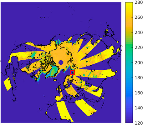
FIGURE 3. Example evening CETB SMAP radiometer vertically-polarized (v pol) T_B image processed with rSIR on an EASE2 map grid for day of year 091, 2015. Open ocean appears cold (low T_B) compared to land, glacial ice, and sea ice. The thick red box to the right of and below center outlines the study area.

FIGURE 4

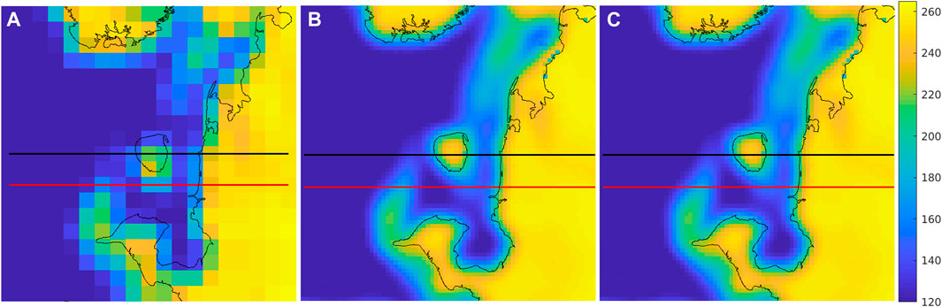
FIGURE 4. Average of daily SMAP vpol T_B images over the study area (see Figure 3) spanning days of year 91–100 with a coastline (Wessel and Smith, 2015) overlay. (A) 36 km GRD. (B) 9 km L1C_TB_E. (C) 3 km rSIR. Note the apparent offset of the island in the GRD, which results from the coarse pixels. The thick horizontal lines show the data transect locations where data is extracted from the image for analysis. The black line is the “island-crossing” case while the red line is the “coastline-crossing” case.

Two horizontal transects of the study region are considered in separate cases. One crosses the island and the coast, while the second crosses a patch of sea ice and the coast, see Figure 4. Due to the dynamics of the sea ice that is further from the shore, only the near-coast region is considered. For simplicity, we model the surface brightness temperature as essentially constant with different values over land and water.

Figure 4 compares 10-day averaged daily GRD, rSIR, and L1C_TB_E images of the study region. In these images, the cooler (darker) areas are open ocean. Land areas have high temperatures, with sea-ice covered areas exhibiting a somewhat lower T_B. The GRD images are blocky, while the high resolution images exhibit finer resolution and more accurately match the coastline. These images were created by averaging 10 days of daily T_B images in order to minimize noise-like effects due to (1) T_B measurement noise and (2) the effects of the variation in measurement locations within each pass and from pass to pass. The derived PSRF and linear resolution thus represent temporal averages. The derived PSRFs are representative of the single-pass PSRFs.

Examining Figure 4 we observe that the ocean and land values are reasonably modeled by different constants, with a transition zone at the coastline. It is evident that the GRD images are much blockier than the L1C_TB_E and rSIR images. This is due to the finer grid resolution of the enhanced resolution images and their better effective resolution. Due to the coarse quantization of the GRD image, the island looks somewhat offset downward, whereas the L1C_TB_E and rSIR images better correspond to the superimposed coastline map.

Figure 5 plots the image T_B value along the two study transects. Note that rSIR T_B values have sharper transitions from land to ocean than the GRD images, and that the GRD image underestimates the island T_B. The GRD values also have smoother transitions than L1C_TB_E and rSIR and overestimate T_B in the proliv Pomorskiy strait separating the island and coastline south (right) of the island. The rSIR curves appear to exhibit a small under- and over-shoot near the transitions compared to the L1C_TB_E images.

FIGURE 5

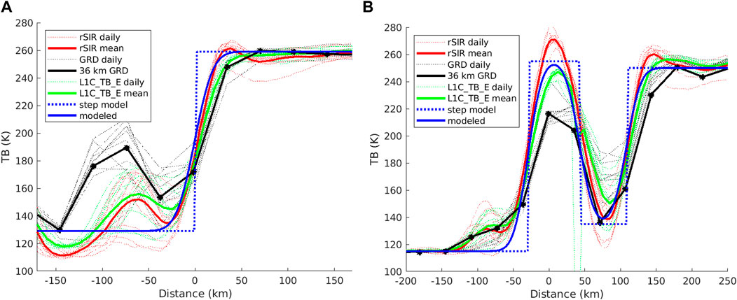
FIGURE 5. Plots of T_B along the two analysis case transect lines shown in Figure 4 for the (A) coastline-crossing and (B) island-crossing cases. Daily values over the study period are shown as thin lines. The curves from the average images are shown as thick lines. The discrete step and convolved Gaussian step models are also shown. The x-axis is centered on the coastline or island center for the particular case.

Lacking high resolution true T_B maps, it is difficult to precisely analyze the accuracy and resolution of the images. However, we can employ signal processing considerations to infer the expected behavior of the values and hence the effective resolution. For analyzing the expected data behavior along these transects we introduce a simple step model for the underlying T_B. Noting that the T_B variation over land near the coast for the coastline case is essentially constant with a variation of no more than a few K, we model the land as a constant. Similarly, the ocean T_B is modeled as a constant. This provides a simple step function model for T_B for the coastline. The island-crossing case is similarly modeled but includes a rect corresponding to the island. The modeled T_B is plotted in Figure 5 for comparison with the observed and reconstructed values. The modeled T_B is filtered with a 36 km Gaussian response filter, shown in blue, for comparison. The latter represents an idealized result, i.e., what can be achieved from the model assuming a Gaussian MSRF.

Examining Figure 5 we confirm that L1C_TB_E and rSIR images have sharper transitions than the GRD images and the GRD image underestimates the island T_B. The GRD images, which have longer ocean-side transitions than L1C_TB_E and rSIR, underestimate the island T_B, and overestimate T_B in the proliv Pomorskiy strait separating the island and coastline south (right) of the island. The ripple artifacts in the rSIR T_B transition from ocean to land in both examples are the result of the implicit low-pass filtering in the reconstruction. The pass-to-pass variability in the T_B observations is approximately the same for all cases in most locations, suggesting that there is not a significant noise penalty when employing rSIR reconstruction or L1C_TB_E optimal interpolation for SMAP.

Insight can be gained by examining the spectra of the signal. Figure 6 presents the wavenumber spectra of the key signals in Figure 7. The spectra were computed by zero padding the data. For simplicity, only the Fourier transforms of the average curves are shown. The spectra of the modeled signal are shown in blue. Peaking at 0 wavenumber, they taper off at higher wavenumbers. The filtered model signal, shown in dark blue, represents the best signal that can be recovered. The GRD signal closely follows the ideal until it reaches the 1/72 km⁻¹ cutoff frequency permitted by the grid, beyond which it cannot represent the signal further. L1C_TB_E and rSIR follow the ideal signal out to about 1/36 km⁻¹ then track each other out to the 1/18 km⁻¹ cutoff for the L1C_TB_E sampling. The rSIR continues out to the 1/12 km⁻¹ cutoff. Details of high wavenumber response differ between the coastline-crossing and island-crossing cases, but the same conclusions apply.

FIGURE 6

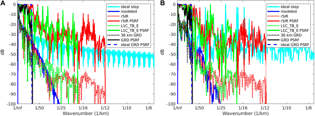
FIGURE 6. Wavenumber spectra of the T_B slices, the model, and the PSRF. (A) Coastline-crossing case. (B) Island-crossing case. See text.

FIGURE 7

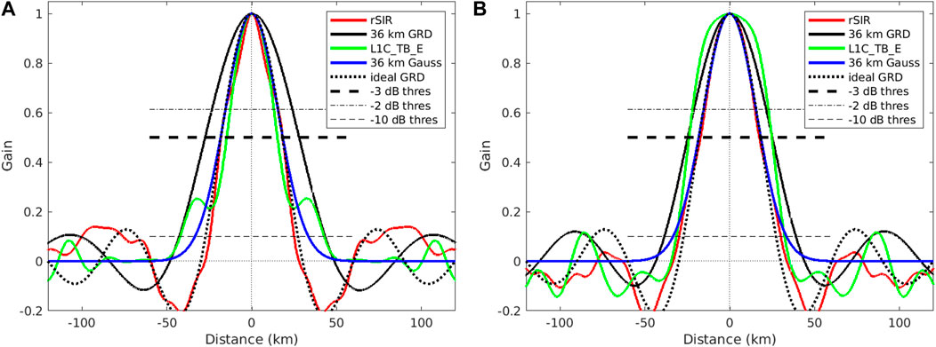
FIGURE 7. Derived single-pass rSIR and GRD PSRFs from the (A) coastline-crossing and (B) island-crossing cases. Shown for comparison are a 36 km wide Gaussian window and a 36 km wide sinc function, which represents the ideal GRD pixel PSRF. The horizontal dashed lines correspond to various thresholds, with the thick dashed line indicating the −3 dB threshold. The effective 3-dB linear resolution is the width of the PSRF at this line.

Deconvolution of the step response is accomplished in the frequency domain by dividing the step response by the spectra of the modeled step function, with care for how zeros and near-zeros in the modeled step function are handled in the inverse operation. The ideal GRD PRSF (blue dashed line) is a rect that cuts off at 1/36 km⁻¹. The estimated GRD PSRF spectrum closely matches the ideal. The rSIR and L1C_TB_E PSRF spectra match the ideal in the low frequency region, but also contain additional information at higher wavenumbers, which gradually rolls off. This additional spectral content provides the finer resolution of rSIR compared to the GRD result.

Finally, the estimated one-dimensional PSRFs are computed as the inverse Fourier transform of the PSRF spectra in Figure 6 as shown in Figure 7. Table 1 shows the linear resolution for each case, computed as the width of the PSRF at the −3 dB point. For comparison, the linear resolutions using both −2 dB and −10 dB thresholds are shown. In all cases the resolution of rSIR is better than the observed GRD resolution.

TABLE 1

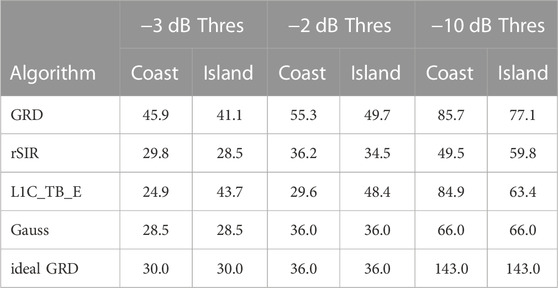
TABLE 1. Inferred linear resolutions from Figure 7 for various algorithms and thresholds.

A key observation is that the effective resolution, as defined by the 3-dB width of the derived PSRFs, is very similar for both analysis cases. As expected, the observed GRD PSRF results are coarser than the ideal GRD PSRF due to the extension of the SMAP MRF outside of the pixel area. rSIR closely follows the ideal GRD and provides a significant improvement over the actual 36 km grid. rSIR is better than L1C_TB_E for the island, but slightly less than L1C_TB_E for the coastline crossing. L1C_TB_E also shows improvement over GRD for the coastline-crossing case, but is slightly worse than GRD for the island-crossing case. The L1C_TB_E PSRF matches the Gaussian-filtered model over the main lobe with small shoulders on the sides of the mainlobe in the coastline case. The rSIR resolution represents a linear resolution improvement of nearly 30% from the observed GRD resolution with a slight improvement over the idealized model resolution. We conclude that rSIR provides finer effective resolution than GRD products, with a resolution improvement of nearly 30%. The resolution enhancement of L1C_TB_E can be similar in some cases, but not all. rSIR provides more consistent effective resolution improvement than L1C_TB_E for the studied cases.

5 Discussion

Regardless of the posting resolution (the image pixel spacing), the effective resolution of the reconstructed T_B image is defined by the PSRF. To avoid aliasing, the posting resolution must be smaller (finer) than the effective resolution. We note that as long as this requirement is met, the posting resolution can be arbitrarily set. Thus the pixel size can be arbitrarily determined based on the pixel size of a standard map projection such as the EASE2 system (Brodzik et al., 2012; Brodzik and Long, 2016).

There are advantages of a finer posting resolution. For example, since the effective resolution can vary over the image due to the measurement geometry, the PSRF is not spatially constant, and to ensure uniform pixel sizes, the image may be over-sampled in some areas. Fine posting ensures all information is preserved and that the Nyquist sampling criterion is met. Furthermore, finer posting provides optimum (in the bandlimited sense) interpolation of the effective information in the image. This interpolation can be better than bi-linear or bi-cubic schemes often used for interpolation in many applications. We also note that fine posting resolution is required by the reconstruction signal processing to properly represent the sample locations and measurement response functions. On the other hand, oversampled images produce larger files and there is potential confusion among users in understanding the effective resolution and adjacent pixel correlation.

When creating the original CETB dataset, Long and Brodzik wanted to ensure that while the different frequency channels have different resolutions which necessitates using different grid resolutions, the grid resolutions are easily related to each other (i.e., by powers of 2) to simplify comparison and the use of the data (Long and Brodzik, 2016). Hence, grid sizes were chosen such that, based on careful simulation, the RMS error in the reconstructed T_B images was minimized subject to choosing from a small set of possible sizes. This analysis is one reason that particular channels are on particular resolution posting grids while their effective resolutions may be coarser–the finer grid provides better error reduction in the reconstruction (Long and Brodzik, 2016).

As previously noted, the ideal PSRF is 1 over the pixel and 0 elsewhere, i.e., a small box car function. However, since we are representing the surface T_B on a discrete grid, we must assume that the signal is bandlimited so that the samples can represent the signal without aliasing. Thus, the bandlimited ideal PSRF is a low-pass filtered rect function, which is a two-dimensional sinc function (Figure 2), though in practice the real PSRF has a wider main lobe and smaller side lobes. Because the PSRF is non-zero outside of the pixel area, signal from outside of the pixel area “leaks” into the observed pixel value. For example, consider a PSRF that is −10 dB at adjacent pixels. If there is an open ocean pixel where the ocean T_B is 160 K adjacent to a land pixel where T_B is 250 K, the PSRF permits the land T_B signal to contribute approximately 9 K to the observed ocean value, essentially raising the observed value to 169 K from its ideal value of 160 K.

As evident in Figure 5, sharp transitions in the surface T_B are under-estimated in all the products. The high resolution products better localize the edge transitions, but may have fluctuations (over- and under-shoot) near the edges, a result of Gibb’s phenomena. The fluctuations can be minimized by filtering or smoothing the data at the expense of the effective spatial resolution but are not entirely eliminated even for the low resolution GRD data. These error values result in errors in geophysical values inferred from the estimated T_B. The error tolerance is dependent of the application of the estimated geophysical values and may vary by user and application. Fine resolution requires tolerance to fluctuations near sharp edges.

The fact that the PSRF is non-zero outside of the pixel area also means that nearby pixels are statistically correlated with each other–they are not independent even in the ideal case. The correlation is even stronger when the effective resolution is coarser than the posting resolution. This effect may need to be considered when doing statistical analysis of adjacent pixels.

6 Conclusion

This paper considers the effective resolution of conventional- and enhanced-resolution SMAP T_B image products available from the NASA-sponsored CETB ESDR project (Brodzik et al., 2021) and the SMAP project L1C_TB_E product (Chaubell et al., 2016; Chaubell et al., 2018). These products include conventionally processed (GRD) gridded images and rSIR and BG optimal interpolation enhanced-resolution images. To evaluate and compare the resolutions of the two products the step function response is derived from coastline and island transects in SMAP T_B images. From these, the effective resolution is determined by computing the average PSRF. As expected, the effective resolution is coarser than the pixel posting (spacing) in all cases. From Tab. 1, the effective 3-dB resolution of conventionally processed (GRD) data, which is posted on a 36 km grid, is found to be approximately 45.9 km, while the effective resolution of the rSIR daily enhanced-resolution images is found to be 29.8 km, which is nearly a 30% improvement. The resolution improvement of L1C_TB_E can be nearly as high at times but is less consistent. The results verify the improvement in resolution possible for daily SMAP T_B images using the rSIR algorithm.

Data availability statement

The datasets presented in this study can be found in online repositories. The names of the repository/repositories and accession number(s) can be found in the article/Supplementary Material.

Author contributions

DL was responsible for the conception and design of the study. MB arranged for funding. DL wrote the first draft of the manuscript. MB and MH edited the manuscript. All authors contributed to manuscript revision, read, and approved the submitted version.

Funding

The funding for this research was provided under NASA grants NXX16AN02G and 80NSSC20K1806 at University of Colorado at Boulder and NNX16AN01G at Brigham Young University.

Conflict of interest

The authors declare that the research was conducted in the absence of any commercial or financial relationships that could be construed as a potential conflict of interest.

Publisher’s note

All claims expressed in this article are solely those of the authors and do not necessarily represent those of their affiliated organizations, or those of the publisher, the editors and the reviewers. Any product that may be evaluated in this article, or claim that may be made by its manufacturer, is not guaranteed or endorsed by the publisher.

References

Backus, G., and Gilbert, J. (1967). Numerical applications of a formalism for geophysical inverse problems. Geophys. J. R. Astronomy Soc. 13, 247–276. doi:10.1111/j.1365-246x.1967.tb02159.x

CrossRef Full Text | Google Scholar

Backus, G., and Gilbert, J. (1968). The resolving power of gross earth data. Geophys. J. R. Astronomy Soc. 16, 169–205. doi:10.1111/j.1365-246x.1968.tb00216.x

CrossRef Full Text | Google Scholar

Berg, W., Kroodsma, R., Kummerow, C., and McKague, D. (2018). Fundamental climate data records of microwave brightness temperatures. Remote Sens. 10, 1306. doi:10.3390/rs10081306

CrossRef Full Text | Google Scholar

Brodzik, M., Billingsley, B., Haran, T., Raup, B., and Savoie, M. (2014). Correction: M.J. brodzik, et al., EASE-Grid 2.0:incremental but significant improvements for Earth-gridded data sets. ISPRS Int. J. Geo-Information 3, 1154–1156. doi:10.3390/ijgi3031154

CrossRef Full Text | Google Scholar

Brodzik, M., Billingsley, B., Haran, T., Raup, B., and Savoie, M. (2012). EASE-Grid 2.0:incremental but significant improvements for Earth-gridded data sets. ISPRS Int. J. Geo-Information 1, 32–45. doi:10.3390/ijgi1010032

CrossRef Full Text | Google Scholar

Brodzik, M., and Long, D. (2016). Calibrated passive microwave daily EASE-Grid 2.0 brightness temperature ESDR (CETB): Algorithm theoretical basis document. Boulder, CO: National Snow and Ice Data Center NSIDC.

Google Scholar

Brodzik, M., Long, D., Hardman, M. A., and Armstrong, R. (2018). MEaSUREs calibrated enhanced-resolution passive microwave daily EASE-Grid 2.0 brightness temperature ESDR. version 1. doi:10.5067/MEASURES/CRYOSPHERE/NSIDC-0630.001

CrossRef Full Text | Google Scholar

Brodzik, M., Long, D., Hardman, M. A., and Armstrong, R. (2021). SMAP radiometer twice-daily rSIR-enhanced EASE-Grid 2.0 brightness temperatures. version 2.0. doi:10.5067/YAMX52BXFL10

CrossRef Full Text | Google Scholar

Chaubell, J., Chan, S., Dunbar, R., Peng, J., and Yueh, S. (2018). SMAP enhanced L1C radiometer half-orbit 9 km EASE-Grid brightness temperatures. version 2. doi:10.5067/0DGGEWUC6MLY

CrossRef Full Text | Google Scholar

Chaubell, J. (2016). SMAP algorithm theoretial basis document: Enhanced L1B radiometer brightness temperature product. Pasadena, CA: Jet Propulsion Laboratory.

Google Scholar

Chaubell, J., Yueh, S., Entekhabi, D., and Peng, J. (2016). “Resolution enhancement of SMAP radiometer data using the Backus Gilbert optimum interpolation technique,” in IEEE International Geoscience Remote Sensing Symposium, Beijing, China, 10-15 July 2016 (IEEE), 284–287.

CrossRef Full Text | Google Scholar

Early, D., and Long, D. (2001). Image reconstruction and enhanced resolution imaging from irregular samples. IEEE Trans. Geoscience Remote Sens. 39, 291–302. doi:10.1109/36.905237

CrossRef Full Text | Google Scholar

Entekhabi, D., Njoku, E., O’Neill, P., Kellogg, K., Crow, W., and Edelstein, W. (2010). The soil moisture active passive (smap) mission. Proc. IEEE 98, 7040716. doi:10.1109/JPROC.2010.2043918

CrossRef Full Text | Google Scholar

Long, D., Brodzik, M., and Hardman, M. (2019). Enhanced resolution SMAP brightness temperature image products. IEEE Trans. Geoscience Remote Sens. 57, 4151–4163. doi:10.1109/TGRS.2018.2889427

CrossRef Full Text | Google Scholar

Long, D., and Brodzik, M. (2016). Optimum image formation for spaceborne microwave radiometer products. IEEE Trans. Geoscience Remote Sens. 54, 2763–2779. doi:10.1109/tgrs.2015.2505677

PubMed Abstract | CrossRef Full Text | Google Scholar

Long, D., and Daum, D. (1998). Spatial resolution enhancement of SSM/I data. IEEE Trans. Geoscience Remote Sens. 36, 407–417. doi:10.1109/36.662726

CrossRef Full Text | Google Scholar

Long, D., and Franz, R. (2016). Band-limited signal reconstruction from irregular samples with variable apertures. IEEE Trans. Geoscience Remote Sens. 54, 2424–2436. doi:10.1109/tgrs.2015.2501366

CrossRef Full Text | Google Scholar

McLinden, M., Wollack, E., Heymsfield, G., and Li, L. (2015). Reduced image aliasing with microwave radiometers and weather radar through windowed spatial averaging. IEEE Trans. Geoscience Remote Sens. 53, 6639–6649. doi:10.1109/tgrs.2015.2445100

CrossRef Full Text | Google Scholar

Meier, W., and Stewart, J. (2020). Assessing the potential of enhanced resolution gridded passive microwave brightness temperatures for retrieval of sea ice parameters. Remote Sens. 12, 2552. doi:10.3390/rs12162552

CrossRef Full Text | Google Scholar

Piepmeier, J., Focardi, P., Horgan, K., Knuble, J., Ehsan, N., Lucey, J., et al. (2017). SMAP L-band microwave radiometer: Instrument design and first year on orbit. IEEE Trans. Geoscience Remote Sens. 55, 1954–1966. doi:10.1109/TGRS.2016.2631978

PubMed Abstract | CrossRef Full Text | Google Scholar

Piepmeier, J., Mohammed, P., Amici, G. D., Kim, E., Pen, J., and Ruff, C. (2014). Algorithm theoretical basis document: SMAP calibrated, time-ordered brightness temperatures L1B_TB data product algorithm theorecial basis document: Enhanced L1B radiometer brightness temperature product. Pasadena, CA: Jet Propulsion Laboratory.

Google Scholar

Poe, G. (1990). Optimum interpolation of imaging microwave radiometer data. IEEE Trans. Geoscience Remote Sens. 28, 800–810. doi:10.1109/36.58966

CrossRef Full Text | Google Scholar

Skou, N. (1988). “On the sampling in imaging microwave radiometers,” in IEEE International Geoscience Remote Sensing Symposium, Edinburgh, UK, 12-16 September 1988 (IEEE), 17–18.

Google Scholar

Ulaby, F., and Long, D. (2014). Microwave radar and radiometric remote sensing. Ann Arbor, Michigan: University of Michigan Press.

Google Scholar

Wessel, P., and Smith, W. (2015). A global, self-consistent, hierarchical high–resolution geography database. J. Geophys. Res. Atmos. 3, 4. doi:10.1029/96JB00104

CrossRef Full Text | Google Scholar