 Vanessa Lucieer
 Emma Flukes
 John P. Keane
 Scott D. Ling
 Amy W. Nau
 Victor Shelamoff
- 1Institute for Marine and Antarctic Studies, University of Tasmania, Hobart, TAS, Australia
- 2Commonwealth Scientific and Industrial Research Organisation, Hobart, TAS, Australia
Robust definition of the spatial extent of seafloor habitats and how they may be changing through time is a holy grail for ecosystem management, particularly if an ecosystem is approaching a tipping point beyond which irreversible changes may occur. Here we generate and explore a new data set for the management of warming reefs in eastern Tasmania, Australia that will significantly improve the baseline maps required for fine-scaled spatial modelling and management that is, both robust at regional scales and is highly resolved within the water column. This procedure enabled the relative density of kelp vegetation to be identified in a region that is being overwhelmed by the range extension of a destructive grazer, the Longspined Sea Urchin, Centrostephanus rodgersii. We present a new online tool to visualize multibeam water column acoustic data as surfaces of kelp density at high resolution (50 cm) scale over seafloor terrain maps (spanning a total straight-line distance of 594 km and a total area of 29.14 km2) to reveal the types of reef structure on the East Coast of Tasmania where abalone habitat is threatened by kelp loss.
Introduction
Kelp beds are among the most productive ecosystems on earth and support high levels of marine biodiversity and valued fisheries (Steneck et al., 2002; Pessarrodona et al., 2022). At a global scale they are increasingly threatened by catastrophic phase shifts to poorly productive sea urchin barrens largely devoid of seaweed cover (Ling et al., 2015) or to turf algae assemblages dominated by low-growing filamentous or branching algal species (Strain et al., 2014). The proliferation of either degraded state (barrens or turfs) would result in a decline in reef fisheries productivity and biodiversity of coastal reef systems and compromise the associated ecosystem services (Ling, 2008). Thus, the ability to map and predict changes in kelp cover is critically important in coastal management. In eastern Tasmania, Australia, a catastrophic shift of kelp bed habitats (dominated by Ecklonia radiata) to Longspined Sea Urchin (Centrostephanus rodgersii) barrens is underway, and is one of the most significant threats to the integrity of rocky reef ecosystems that support valuable rock lobster and abalone fisheries (Johnson et al., 2005). This range-extending destructive grazer of kelp beds has invaded eastern Tasmania via increasing southerly incursions of the East Australian Current (EAC), creating ecologically and fisheries depauperate barrens for ∼15% of reef (5–40 m depth) along the east coast of Tasmania (Ling and Keane, 2018). Effective management of this problem is contingent on highly resolved spatial data defining the extent and type of reef systems currently impacted by urchins, including areas vulnerable to future overgrazing (Ling and Keane, 2021; Keane et al., 2022).
The reef systems on the east coast of Tasmania were first mapped at low resolution using single beam sonar acoustics (>50 m scale) between 2001 and 2009 by the Seamap Tasmania project (Lucieer et al., 2007; Lucieer et al., 2009). These interpolated maps define the reef and sand boundaries and the extent of the reef systems, but not the fine scale internal physical structure which has been identified as a key element in the susceptibility of reef systems to recruitment and establishment of Centrostephanus (Ling and Johnson, 2012). Currently marine managers rely on these low resolution, interpolated habitat maps and kelp cover maps derived from a series of spatially nested diver and video transects downscaling from ∼25 km to 2 km along the coast of Tasmania (Ling and Keane, 2018). Traditional diver and video based transect methods for surveying habitat coverage are laborious, expensive, and more spatially limited in mapping the underwater environment compared to acoustic surveys nor are they at sufficiently high resolution to map fine-scale reef structure. Nevertheless, diver and video-based techniques have been used to document the broad-scale decline in the cover of canopy-forming kelp along the east coast of Tasmania associated with the dramatic expansion of Centrostephanus barrens (Ling and Keane, 2018) and notably remain the only way to effectively track growing populations of urchins within kelp beds (Ling et al., 2016). Appropriate integration of these two approaches—high resolution acoustics and diver-and-video-based surveying—can provide much needed and valuable information to managers, e.g., defining the influence of vegetation loss on catch rates of commercially important species (Young et al., 2016). Furthermore, it could optimise the use of limited resources and permit the opportunity to identify where targeted surveillance of urchins and kelp with intensive diver surveys should be conducted.
Multibeam acoustic methods can be employed to survey the seabed at high resolution (<1 m scale) and also collect coincident water column data, that is comparable in scales to diver-based video surveys. The water column acoustic record enables the identification of ecological features that extend into the water column. This improved spatial resolution of water column data collected from acoustic multibeam systems has only become possible because of availability of complex computing power that this method relies on, but also in new acoustic methods being developed (Schimel et al., 2020; Nau et al., 2022; Porskamp et al., 2022). One of these developments includes new filtering algorithms to reduce the feature space of acoustic targets in the water column and refine the analysis to the features of interest such as isolating those points that are within 1 m distance of the seafloor, similar to the methods identified by Porskamp et al. (2022). This provides us with a means to be able to differentiate reef that hosts vegetation from reef that is barren—presenting us with a method to map urchin barrens over a greater area than is viable from video diver transects alone (Porskamp et al., 2022). In this study the seafloor acoustic signal was processed at 50 cm resolution and classified using the Seamap Australia classification scheme (Lucieer et al., 2019)—into pavement reef, megaclast reef, mixed hard substrata and sand. To cross-calibrate the water column signal of macroalgae and to establish a baseline of the size-frequency of barrens patches across eastern Tasmania we conducted video surveys simultaneously alongside acoustic mapping. Video footage was annotated at the scale of individual barrens and kelp patches to quantify their current patchiness, and importantly identify the earliest stages detectable for incipient barrens (barrens <5 m in diameter).
We present a new water column mapping method that has been operationalized for management surveys of reef systems in <20 m depth to create a spatially continuous dataset of rocky reef structure, extent and coverage of reef associated vegetation using multibeam sonar water column data. This dataset presents a stepwise improvement on video transect survey methods because there are no “gaps” in the survey data, eliminating the potential for under or over representation of barrens from systematic spacing of sites every ∼20 km. This data provides a resource for describing, modelling, and predicting the distribution of kelp habitat and, through the absence of kelp, indicate where urchin barrens may be present along Tasmania’s climate change impacted east coast. The unprecedented high resolution (50 cm) maps of the reef structure will improve the ongoing management of Tasmania’s kelp bed habitat and the associated fisheries by underpinning stock assessments and providing a high-resolution data set that can be used in prediction modelling of where kelp habitat may be at risk-ultimately improving the spatial knowledge of these reefs for key species.
Materials and methods
Multibeam acoustic data and coincident video transects were sampled along the East Coast of Tasmania covering seven of fifteen fishing blocks (blocks 22 to 30, excluding blocks 25 and 26) most heavily impacted by Centrostephanus in the Eastern Zone of the Tasmanian Abalone Fishery (Ling and Keane, 2018; Mundy and McAllister, 2021). The fishing blocks geographically delineate the regions open for fishing for commercial harvest. Abalone harvest from the Eastern Zone peaked at 1,500 t in 1998, but has decreased to 220 t in 2020 with stressors on stock including overfishing, climate change, marine heat waves, as well as habitat loss from urchins (Mundy and McAllister, 2021).
Acoustic acquisition and seafloor data processing
Field surveys to collect multibeam acoustic data were conducted between Eddystone Point to Tasman Island between the 17th and 21st of April 2021, when we expected seasonally high kelp canopy cover (Layton et al., 2020). The extent of the survey spanned abalone management blocks 22, 23, 24, 27, 28, 29, and 30 which are further divided into sub blocks as shown in Figure 1A. A Kongsberg Maritime EM2040 multibeam sonar was pole mounted on the RV Abyss (Marine Solutions) vessel. The multibeam sonar collected swath data at an average width of 50 m across the surveyed depth range of 10–20 m. CARIS HIPS and SIPS software was used to process the bathymetric data into a bathymetric gridded surface at 50 cm resolution. The bathymetric surface was analysed in ArcGIS 10.8.1 to produce spatial derivatives of seabed slope, planform curvature, and topographic position index.
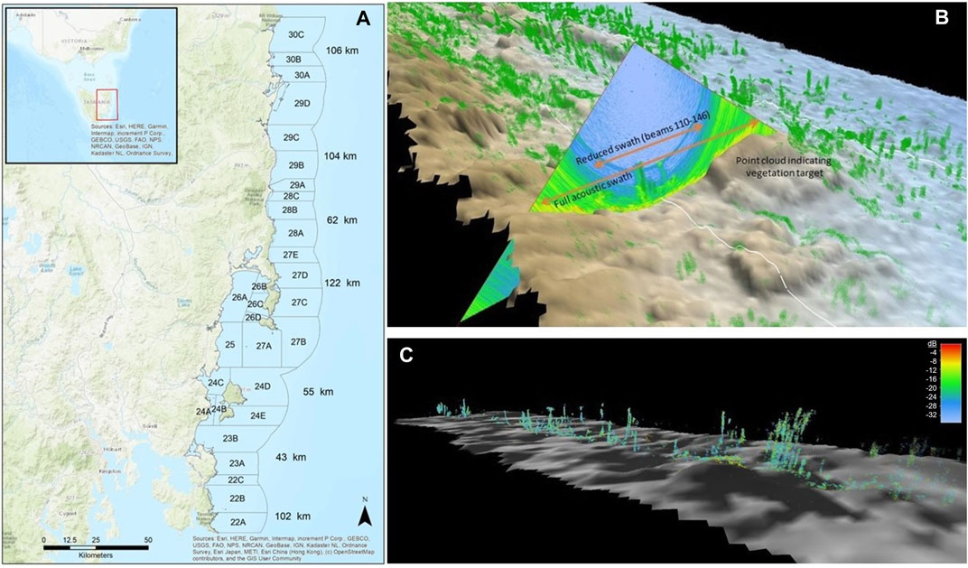
FIGURE 1. (A) Numbered fisheries management blocks for the abalone industry on the east coast of Tasmania. Each block shows linear distance of survey transect in <20 m water depth. (B) Multibeam acoustic swath visualised over the benthic terrain model. Green point cloud indicates features that were extracted from the water column. (C) The remaining point cloud could be filtered by dB to extract estimates of signal strength which relates to vegetation density.
The bathymetric surface of the seafloor was analysed to generate habitat maps depicting reef type. Substratum type was inferred using an unsupervised classification approach based on a raster stack of depth, slope (calculated on a neighbourhood of 4), planform curvature (based on a scale factor of 9), a zero corrected topographic position index (based on a circular window scale of 5) and a non-zero corrected topographic position index (based on a circular window scale of 9). These derived bathymetric products were calculated using Raster package in R (https://cran.r-project.org/web/packages/raster/index.html). The ‘unsuperClass()’ function in the RStoolbox package in R (https://www.rdocumentation.org/packages/RStoolbox/versions/0.2.6) was used to classify each management reporting block into 5 classes based on “MacQueen” algorithm drawn from 10,000,000 random samples and run over 10,000 iterations. The five classes represented pavement reef, megaclast reef (boulder reef), mixed hard substrata and two depth strata of sand (<15 m and >15 m). This assisted in better defining the mixed hard substrata category. The final habitat classification consolidated the two sand categories into one-resulting in 4 classes in total.
Acoustic water column feature extraction
The water column data from the multibeam data record (all and.wcd format) were read into Matlab using the open-source CoFFee toolbox (https://github.com/alexschimel/CoFFee). The water column samples were filtered using subsequent custom Matlab scripts based on Nau et al. (2022) to eliminate most of the unwanted noise while retaining targets likely to be signal from vegetation (Figure 1B). Figure 1C shows that the filtering algorithm permitted the assessment of ‘targets’ close to the seafloor to be retained limiting only those points within 1 m of the seafloor.
The first steps were to remove the high amplitude signals from the seafloor using a model to estimate the spreading of the seafloor signal across all beams, as well as an amplitude threshold to remove residual spreading from sharp rocky features. The across-track sidelobe noise was filtered using a threshold calculated from the raw sample amplitudes (dB) from each sample range equal to the mean plus two times the standard deviation of all samples along that sample range (Figure 2A) (Nau et al., 2022). A final threshold filter of −30 dB was applied to remove remaining low amplitude noise (Figure 2B). Only targets within 1 m of the seafloor were retained to eliminate mid-water targets. An along-track sidelobe filter was used to remove any signal below the modelled spreading of along-track sidelobe interference due to rocky seafloor features using the methods described in (Nau et al., 2018). This step removes data surrounding large rocky features. Final analysis was limited to the inner 36 beams (beams 110–146) due to the high signal noise created by rocky reef environments in the outer beams.
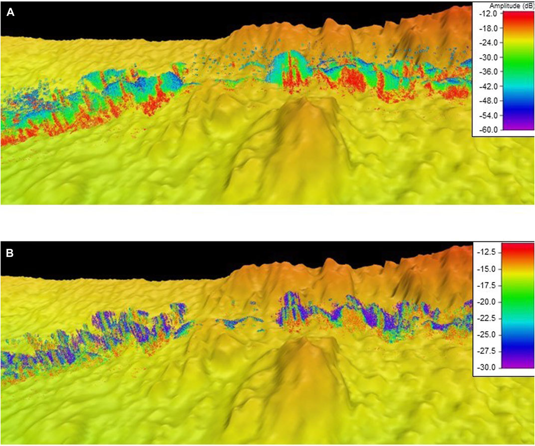
FIGURE 2. (A) Kelp (in red) can be seen in the acoustic swath (no threshold). (B) When a threshold is applied to the signal it removes excess “noise” and permits higher resolution of the vegetation to be detected, improving the accuracy of the classification.
The remaining signals were gridded by calculating the average signal within 50 cm grid cells and exporting as point features at 50 cm spacing (Figure 2B). In ArcGIS, these points were re-gridded to 1 m resolution using the mean signal within 1 m blocks. The Block Statistic tool was run using a 3 × 3 neighbourhood and calculating the mean value to create a surface representing 9 m2, which we deemed to be a relevant scale for managers to enact management decisions (e.g., enact urchin control before collapse to extensive barrens occurs). The presence of small barrens patches (1–10 s square metres) within kelp beds is not problematic for fisheries production or biodiversity more generally but are seen as early warning signs for more extensive barren formation (Ling and Keane, in prep). Urchin barrens become problematic when the sea urchin’s abundance builds towards the tipping-point of overgrazing (approx. 2.0 urchins per m2) across hectares to hundreds of hectares of the reef, when collapse to extensive barrens occurs (Ling et al., 2015; Ling and Keane, 2018).
The raster layer “block statistic” was then reclassified using a threshold to make a “traffic light” quick reference map with three classes representing-bare (no signal in the water column), patchy (medium level signal) and dense signal (lots of vegetation). The thresholds for the three classes were −64 (minimum) to −60 db as bare, −60 to −50 as patchy vegetation, and >−50 as dense vegetation. The geotiff layers were uploaded onto the Seamap data portal as three different files: the 1 m mean signal, the raw “block statistic layer” of mean dB (9 m2), and the threshold ‘traffic light’ layer. The water column data was then analysed in relation to the reef classes using a raster statistic (Figure 3).
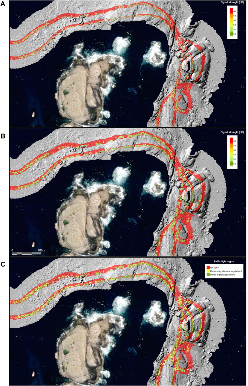
FIGURE 3. Water Column Data (WCD) overlaid on 50 cm hillshade at Governor Island Marine Reserve. Panels show: (A) WCD 1 m2 continuous surface; (B) WCD 9 m2 mean signal; and (C) thresholded vegetation likelihood “traffic light signal.”
Video data collection and analysis
Video collection and annotation
At sites within key abalone blocks (Blocks 22/23 –Tasman, Block 24—Maria, Block 27—Freycinet, Blocks—29/30 St Helens) acoustic mapping was supplemented with the simultaneous deployment of towed underwater video. GPS positions for the towed video system were acquired using a TrackLink 1500 USBL tracking system with a spatial accuracy of less than 1 m. These blocks were chosen as prior diver and towed-video surveys revealed a range of urchin densities and overgrazing impacts from metre-scale incipient barrens up to barrens 100 sm in length (Ling and Keane, 2018).
The video footage was annotated at the scale of individual kelp and urchin barren patches, whereby the start and end points of discrete patches of canopy-forming kelp and urchin barren were recorded as precisely as possible with the assistance of Biigle video analysis software (https://biigle.de). Three different types of barren patch were identified based on the percentage of barren reef within the camera’s field of view (∼3–4 m). Dense, middle, and sparse barren categories represented barrens with >85%, 40%–85%, and <40% cover respectively. Different types of kelp patches were identified based on the species composition and density of the canopy strata. The different kelp density categories (also assessed relative the camera’s field of view) identified were dense: representing >60% cover, middle: representing 20%–60% cover, sparse: representing <20% cover. The start and end points of regions of sand and uncategorisable sections of video (sections of poor visibility of the benthos or titled camera angles) were also annotated so that these sections could be excluded from subsequent analyses. The position of the start and end points of the annotations in the video were determined based on the time-calibrated position of the towed camera, allowing for the distance across all barren patches to be calculated.
Barren patch-sizes and cover estimates
The percentage of reef distance covered by different kelp and barren patches was determined by summing the distance of the algal and barren patch types and dividing by the total distance of reef (i.e., total video distance per transect—all uncategorisable/sandy sections). The percentage of reef covered by complete barren was then estimated by multiplying the percentages of each barren type by the mid-point of its density range i.e., the proportion of reef covered by dense barren was multiplied by 92.5% (the midpoint of 85%–100% cover), consistent with the approach used by Ling and Keane (2018). These percentages were then compared to equivalent data determined by the multibeam survey. The mean size of continuous barren patches and the size spectrum of the different barren patches were plotted to provide a baseline assessment of urchin barren patch dynamics across the variously impacted abalone management sub blocks.
Results
Acoustic water column results
Seafloor habitat data at 50 cm resolution was collected for the abalone blocks 22 to 30 (excluding blocks 25 and 26) consisting of a survey line of 594 km, resulting in 29.14 km2 of high-resolution habitat data. Acoustic bathymetry data derivatives, which describe the characteristics of the reef system, have been extracted and made publicly available on the IMAS Data Repository: https://doi.org/10.25959/AHR1-Q718. These data include the multibeam bathymetry, spatial derivatives of the bathymetry data (seabed slope, curvature, rugosity, and associated contour information), classified benthic habitat maps, point-based video validation data, and acoustic water column data (WCD). The WCD data is supplied in three formats: the first is a continuous surface at 1 m2 resolution that illustrates the range of dB values for targets detected within the water column. Those targets that were not within range of 1 m of the seafloor were removed from the point cloud on the assumption that they were either bubbles or fish. The dB values are displayed as a continuous range from −10 to −64 dB with the lower values showing low signal and the higher values showing greater signal. The 9 m2 resampled version of the product reflects the scale at which the accuracy of the video data was collected and was used for the “traffic light” vegetation density thresholded product. An example for the seafloor from Governor Island Marine Reserve is shown in Figure 3. The entirety of the survey data can be visualised on the Seamap Australia data portal at https://tiny.cc/mappingwarmingreefs.
Table 1 shows that, at the shallowest sampling depth of ∼3 m, the occurrence of no signal, moderate signal, and dense WCD signal strengths were approximately equal. By excluding sand (and analysing the acoustic signal on hard substrate only) we can examine different vegetation density classes on reefs and infer the likelihood of low vegetation density (Table 2). In deeper waters, “no vegetation” (low signal) was the most prevalent acoustic signal with a maximum depth of 53.1 m, almost 10 m deeper than for ‘vegetation’ acoustic signals (44.9 and 45.1 m for medium and dense signals, respectively). The mean depth for the unvegetated signal was 21.3 m—more than 2m deeper than patchy (19.1 m) and densely vegetated (17.6 m) signals, respectively - and within the range 5–35 m in which empirical observations have indicated urchin barrens to be present. Depth variation in the occurrence of different reef classes may affect vegetation density and likelihood of low acoustic signal strength; Table 3. Table 4 shows the summary results of the likelihood of a vegetation class (bare reef, patchy vegetated reef and dense vegetated reed) by different reef classes (sand excluded).
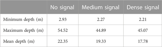
TABLE 1. Depth summaries of WCD signal strength (all substratum types).

TABLE 2. Depth summaries of vegetation density likelihood classes on hard substratum (sand excluded).

TABLE 3. Depth summaries of hard substratum types (sand excluded).
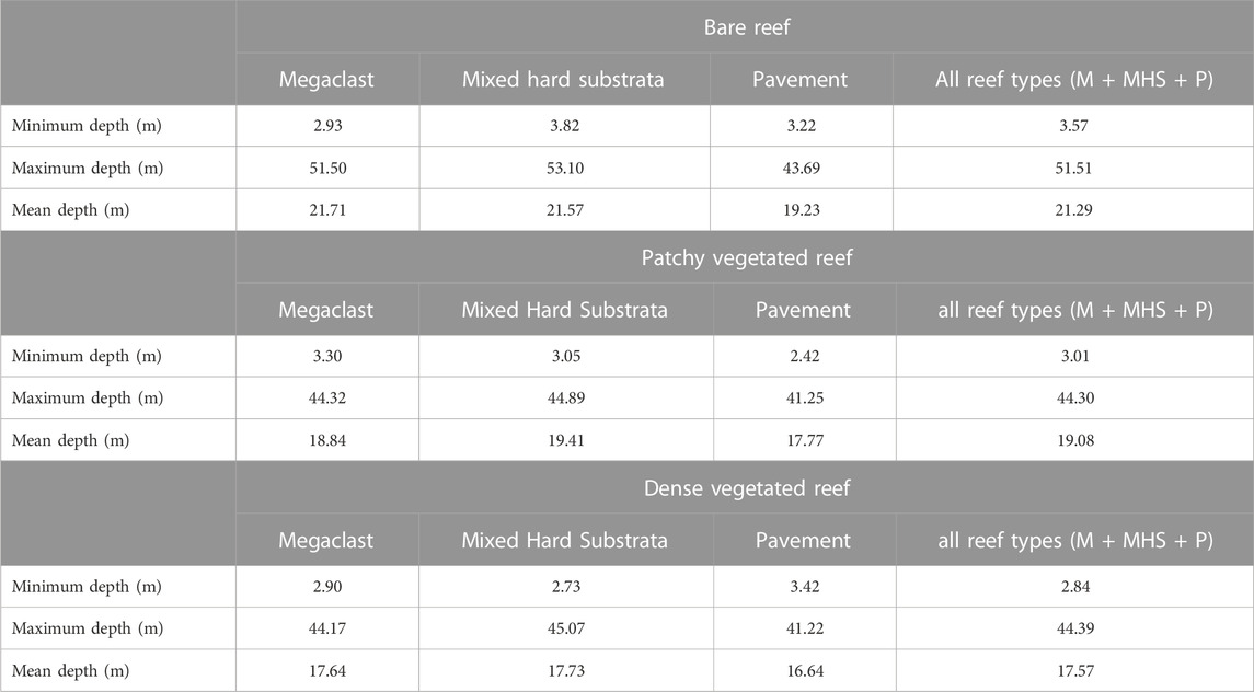
TABLE 4. Depth summaries of vegetation density likelihood classes by reef types.
Figure 4, Table 5 depicts vegetation density and infers the likelihood of urchin barrens occurring depth (in 5 m intervals) and type of hard substratum. If we are to assume that vegetation density reduces at 25 m water depth due to light attenuation and transitions into reef-associated benthic invertebrate communities, a focal depth to examine sea urchin overgrazing of kelp is nominally between 5 and 25 m. Within this range, the highest proportion of likely barrens occurred on mixed hard substrata (73% unvegetated reef within the 20–25 m depth range).
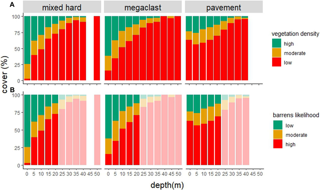
FIGURE 4. Percent cover of (A) different vegetation densities, and (B) inferred barrens likelihood, at different depths (5 m intervals) across different hard substratum types (mixed hard = mixed hard substratum). Lighter shading in b represents depths >25 m for which vegetation density cannot be used to reliably infer the barrens likelihood.
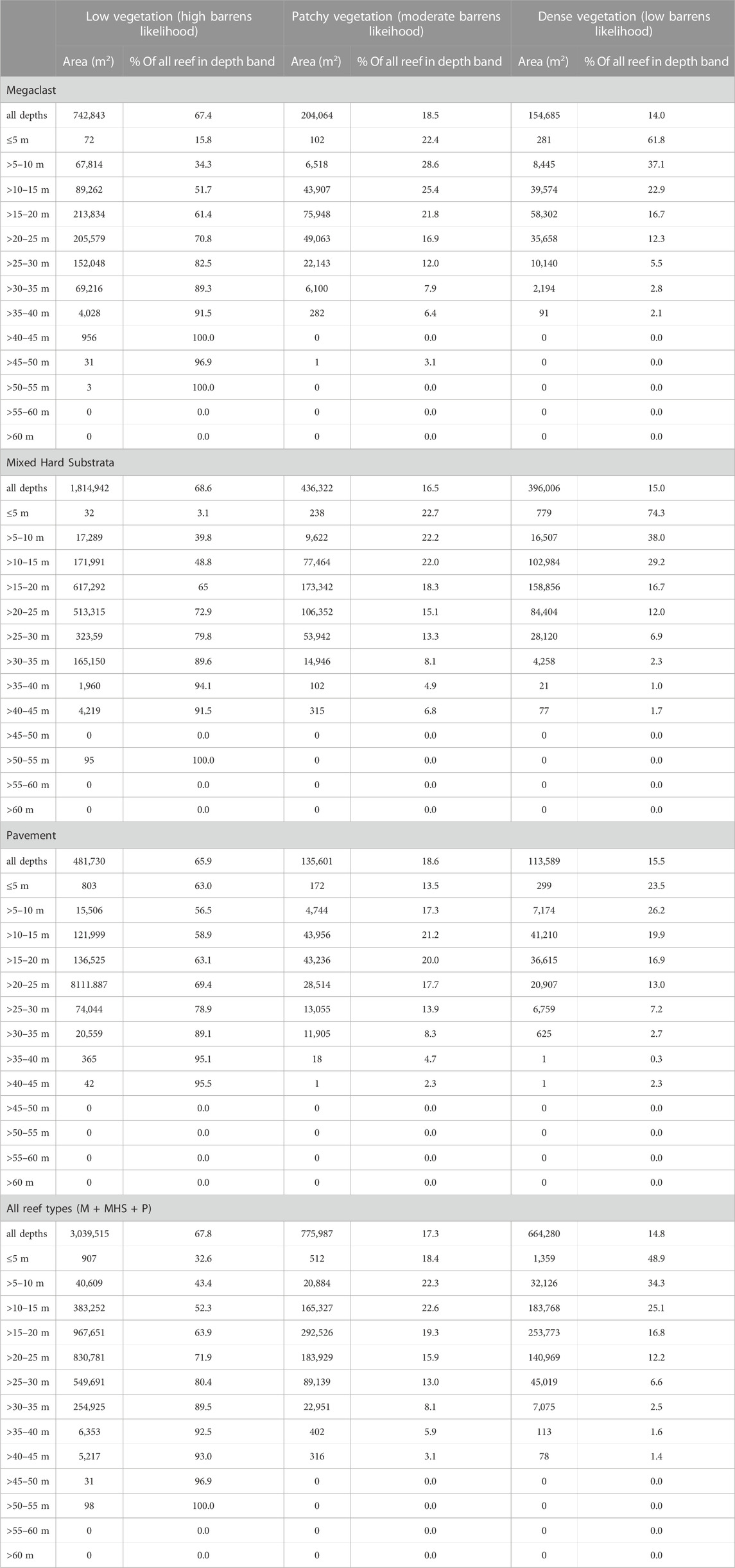
TABLE 5. Occurrence of barrens likelihood classes, by depth (5 m intervals) and hard substratum type (sand excluded).
Video results of barren area and algal canopy cover
Barren and algal canopy cover across sub blocks
The cover of Centrostephanus barrens increased markedly from the less impacted southern sites (sub-blocks 22A, 23B) to the more impacted northern sites (sub-blocks 30A and 30B) from ∼5% complete barren cover to >70% complete barren cover (Figure 5). Conversely, the algal canopy cover transitioned from being relatively complete (although not necessarily dense), to being sparse and very patchy moving from the sites less impacted by Centrostephanus barrens in the south to the more impacted northern sites (Figures 5, 6). This trend was supported by both video (Figure 7A) and acoustic water column (Figure 7B) results. Ecklonia and mixed Ecklonia—Phyllospora beds featured predominantly in the mid-density category dominated reef areas in sub blocks 22A and 23B (Figure 6). These algal canopy types were also a feature of central blocks (blocks 27 and 29) but diminished in extent due to the presence of completely bare (barren) areas of reef. Sub-blocks 27C and 27D also featured some emergent Cystophora growing above the canopy of Ecklonia and Phyllospora, but only rarely. Block 30 was dominated by bare reef substratum (∼70%) and also contained occasional small patches of Ecklonia and mixed Ecklonia and Phyllospora. Across all algal canopy species, dense cover was relatively rare at sub blocks 22A and 23B, despite the absence of bare reef (Figure 6). With the exception of sub-block 27C, dense vegetation comprised a relatively minor (<25%) component of the total area covered by vegetation.
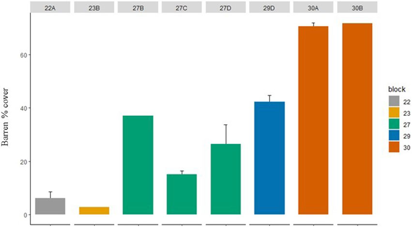
FIGURE 5. Mean (±SE)% of reef estimated to be covered by “complete” barren across abalone management blocks.
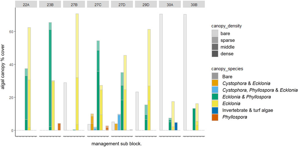
FIGURE 6. Mean% cover of different algal canopy species at different densities across abalone management sub blocks. Bare = no algae, sparse = 0–20%, middle 20%–60%, dense = >60% cover.
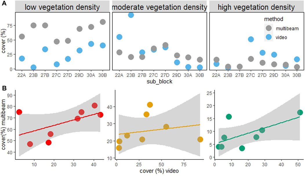
FIGURE 7. % of reef 5–25 m covered by three algal canopy densities across species determined by video and acoustic water column data. (A) is % cover across fisheries management subblocks and (B) is the correlation plots comparing estimates derived from the two survey methods. Low, moderate, and high algal densities represent algal cover of 0–20, 20–60, and >60% respectively determined by video analysis, and signal strengths of −64 to −60 db, −60 to 50, and >−50 respectively determined by the acoustic water column (multibeam) data.
Barren patch size and density across sub blocks
The patch size of Centrostephanus barrens increased markedly from the southern sites (in blocks 22 and 23) to the more impacted northern sites (in block 30) with an approximate 10-fold increase in the mean size of barrens (i.e., 10 m–100 m) (Figure 8A). There was a comparatively low density of barrens at the severely impacted northern sites (sub blocks 30A and 30B), but these barrens tended to be larger in size (i.e., in the 40 m + distance bin). Whilst in the southern sites (sub bocks 22A and 23B) and central sites (sub blocks 27 A, C and D), barrens were more numerous, but they were largely in the <5 m distance bin, although there was a more even spread of barren sizes in the central sites (Figure 8B).
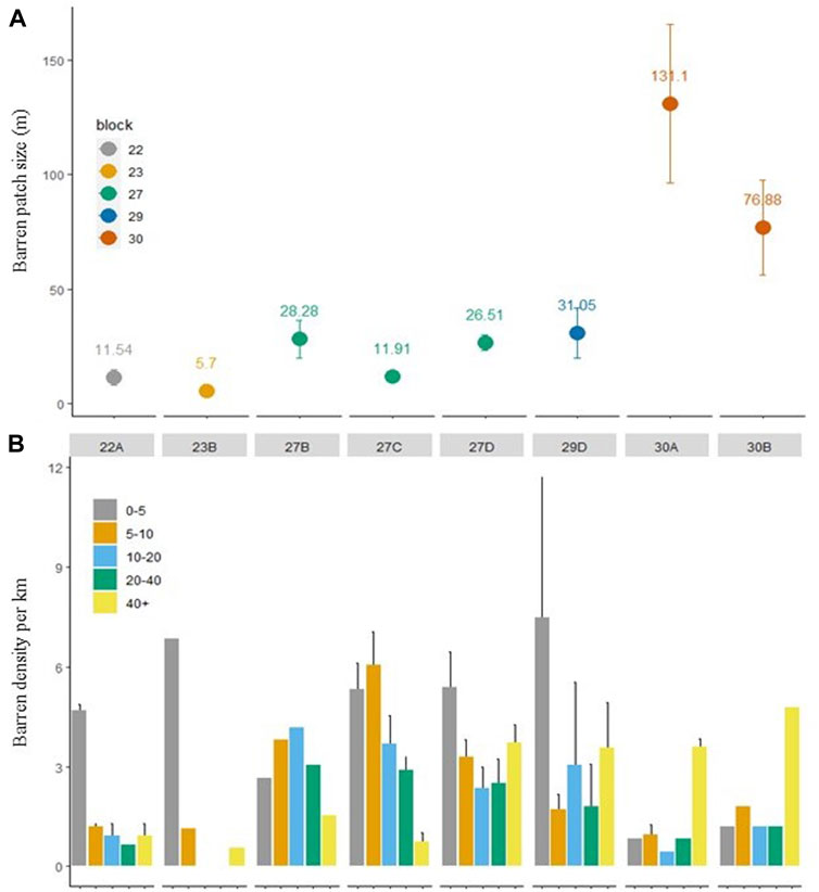
FIGURE 8. Urchin barren patch size and density dynamics. (A) Mean (±SE) of urchin barren patch size (m) based on the length of each barren across abalone management sub-blocks. Numbers above plotted points show the mean patch size in meters. Means and standard errors were generated from the total number of barrens recorded within each sub block. (B) Mean (±SE) density of urchin barrens (number per kilometer of reef) belonging to different size bins (m) grouped by abalone management sub-block based on video surveys in 2020–21. Means and standard errors were generated from n = 1–5 sites within each sub-block.
Discussion
This research has demonstrated an application of acoustic water column data to create a baseline for the extent and condition of kelp vegetation on shallow reef systems in depths <25 m that can be used as a tool for management to monitor vegetation change within abalone fishing administration blocks. The results presented here showing the probability of vegetation on the reef system are useful for rapid assessment of reef vulnerability and have a spatial coverage far greater than is possible from traditional visual surveys. The unprecedented high resolution (50 cm) maps of the reef structure will improve the ability of management to respond to specific kelp bed habitats that are imminently under threat and assist in the triage of allocating resources (for example, urchin management) at an appropriate time. These data will critically underpin spatially explicit “tailored modelling” of changes in kelp habitat and urchin barren development along the east coast of Tasmania as it is impacted by climate change. These data will be of upmost value to decision support tools employed by commercial reef associated fisheries to manage stock assessments, assessing the regional risk of kelp habitat loss and improving knowledge of the function of these reefs for key species.
The results of the video analysis support our ongoing understanding of the extent of the urchin barrens across the Tasmania’s east coast (Ling and Keane, 2018; Ling and Keane, 2021) and additionally provides a detailed description of the spatially dynamic nature of kelp bed and urchin barren patches. In particular, it has documented site-to-site variability in the density of kelp and Centrostephanus barren patches across a spectrum of barren patch-size ranges. The broad-scale pattern in the extent of barren cover, with increasing cover moving from southern sites (blocks 22, 23) to more northern sites (block 30) is consistent with results from 2001 to 2017 survey data presented in Ling and Keane (2018). However, the present estimates of reef occupied by complete barren are up to ∼20% higher than for those estimated in 2017 for the same range of depths (10–20 m) and the same sub blocks. This difference could reflect an increase in the extent of barrens over the 5-year interval between the surveys; however, this notion should be viewed with caution given that different reef areas were surveyed, this survey was not spatially structured, and different video analysis methodologies were used (see Ling and Keane, 2018). A more robust current comparison in the impact of Centrostephanus on east coast reefs would involve the continuation of the sampling/analysis protocol outlined in Ling and Keane (2018); such surveys are due for completion in 2023 (Keane, pers. comm.).
Underwater imagery can be used to map the extent of urchin impact, and through space and time, can be used to gain insights into the patch dynamics of urchin barrens formation within kelp beds (Ling et al., 2016; Williams et al., 2016). Currently though, imagery-based mapping has only focused on defining percentage cover of barrens in broad categories (Ling and Keane, 2018) whereas a full assessment of barrens patch-size distributions as a continuous variable, spanning small (<5 m) to larger (1000 ms) barrens features, has not been conducted. This type of assessment will not only enable patch dynamics to be determined in space and time but will also enable identification of the earliest spatial warnings of impending kelp bed collapse. While useful for identifying broad-scale trends in the extent of kelp beds and urchin barrens, this study revealed a high density of urchin barrens at intermediate patch sizes (5—40 m length) across blocks 27 and 29 (Figure 8A) which is indicative of likely expansion to larger scale barrens in the future as multiple sizeable barrens coalesce (Ling and Keane, 2021). Management intervention at this stage, through targeted harvesting and/or culling, of these areas is paramount before collapse to extensive barrens occurs at which point recovery becomes exceedingly difficult (Ling et al., 2015; Ling et al., 2016; Johnson et al., 2017; Ling and Keane, 2021).
The comparatively low prevalence of dense canopy algae in sub blocks 22A, 23B, and 27B (Figure 6), despite the low abundance of urchin barrens, warrants further exploration, but could be influenced by water temperature, exposure to rough coastal conditions, or differences in substratum type (which is now possible to determine at the sub-block or smaller scale using the high-resolution acoustic data collected by this project). The higher prevalence of dense algal cover at more impacted sites may also be a result of dense localised remnant patches being more resilient to environmental stress and/or grazing by urchins, e.g., on the tops of large boulders or where sand gutters provide barriers to sea urchin movement (Ling pers. obs.). It should also be noted that the greatest difference between the estimated cover from the video surveys and the multibeam survey occurred at blocks 22 and 23, where dense vegetation (>60% cover) was rare, but total cover was 100%; where the reefs were extensively covered in kelp, but predominantly at the lower densities. This may indicate that small macroalgal species (e.g., red and green seaweeds), sponge and macro invertebrate communities, and turf algal communities may not have been detected by the water column acoustics (red and green algae are prevalent in block 22A). This suggests that the multibeam was less able to detect sparse cover kelp compared to mid/dense kelp, which could mean that adjustments in the sensitivity/thresholds used in the data processing are warranted. Given the speed at which the coastline was surveyed using multibeam acoustics (∼3–5 days), this method controls for seasonal variation in sparseness of kelp beds which can impact some diver-based monitoring programs whereby the time taken to survey many sites across >250 km of coastline abridges multiple seasons (or years) given the workload involved.
Through applying a new acoustic water column mapping method, we have been able to assess the effectiveness of hydroacoustics for determining kelp distribution over large scales, and inversely areas of likely urchin barrens (inferred by absence of vegetation). The acoustic water column data analysis illustrates an increasing likelihood of “no vegetation” with depth, which is expected given the natural decrease in vegetation density on temperate reefs with increasing light attenuation. This concurs with empirical observations of kelp communities diminishing and benthic invertebrate communities beginning to dominate with increasing depth for the surveyed region. The high resolution at which the acoustic data was collected enables us to additionally resolve relationships between vegetation density and substratum type that have not previously been possible at such a large spatial scale from visual surveys alone. For example, the presence of “no vegetation” (high likelihood of barrens habitat) occurs, on average, shallower (relative to the mean depth of occurrence of that reef type) on mixed hard substrata compared to other reef types (mean depth of MHS = 23.6 m, mean depth of barrens on MHS = 21.7 m). This supports the observation that barrens occur more readily on complex reef substratum (compared with pavement reef) in which urchins can locate shelter in rocky interstices and feed more readily in rough sea conditions (Flukes et al., 2012; Ling and Keane, 2018). Similarly, patchy vegetation (moderate acoustic signal) becomes less likely in the sub-10 m bracket specifically on pavement substrata. This aligns with our understanding that it is difficult for urchins to initiate forming barrens on flat featureless rock surfaces in shallower areas where water movement is greater. The average depth occurrence of the three reef types however is also different: pavement occurs at shallower depths than megaclast and mixed hard substrata, so caution must be applied in interpreting depth trends by substratum type. This may also be biased by the fact that pavement reef is more prevalent in the north of the extended Centrostephanus range in Tasmania (fishing block 30).
The thresholded “traffic light” data layer indicating the likelihood of the reef system being bare of canopy-forming macroalgae was created by applying three dB thresholds (−64 to −60, −60 to −50 and >−50 as bare, patchy and dense vegetation, respectively) to the continuous 1 m2 layer. These thresholds will require further analysis to determine whether the ranges selected are appropriate for use on different types of reef habitat, and if they can be applied consistently across depths. When examining the point clouds there are quite a few areas where the ringing around the rocks is getting picked up as “kelp,” even though the reef is barren. This is likely due to the ship turning and the along-track noise filter not being able to adequately model the noise pattern around the rocks. We applied the same dB threshold for data on megaclast reef as well as pavement reef or mixed hard substrata. It may be reasonable to assume that the topography affects the water column signal and therefore different thresholds may be more appropriate for different structural complexity. Further research might explore the links between the dB values of the water column with the Vector Ruggedness Measure (VRM) surface to correlate the signal strength against how rugose or flat the reef substratum is. VRM data created from this analysis is available from https://doi.org/10.25959/AHR1-Q718.
This study would benefit from additional high precision video data to improve the ability to resolve the densities in vegetation from the water column data signal. The positioning uncertainty (∼5 m) of the GPS on the video transects impeded our ability to be able to match the acoustic point cloud estimates directly to the imagery which was needed to be able to resolve the density of vegetation. In a preliminary pilot study for this survey, we employed a high precision USBL acoustic positioning system (Sonardyne Mini-Ranger 2 USBL System with Nano Transponder, accurate to within 0.5 m) hired from STR. The cost of the hire of the high precision USBL was not budgeted for this project and therefore could not be employed for the full survey. For future research we recommend only a high precision USBL positioning system be used on the video transects for validation of the water column signal. This has implications for the current data sets and must be considered when interpreting the acoustic data result. The video transect data indicate that there are <5% barrens cover in blocks 22/23, - yet the water column acoustic data reports no signal from 60%–70% of the reef systems. One of the aims of this study was to determine if incipient barrens can be detected. At the scale that incipient barrens occur (<9 m2) we advise that further research would be required to resolve this question. To be able to map low vegetation densities we need a better understanding of the target strength in dB to the biomass of the kelps present on different seafloor rugosities. Although we can detect individual kelp thalli in the acoustic signal in the inner beams, it is difficult to assess, without further study, how the target strength reduces across the swath and what the impact of a rugose (i.e., megaclast) reef habitat has on the water column signal.
Figure 3 shows clear changes in detectability across the acoustic swath, with vegetation (shown in green) largely occurring in the centre of the swath, yellow on the sides of the nadir line (centre line), and red most frequently on the edges of the swath. One of the limitations of this survey has been understanding the angles of dependence across the swath for which the water column results are reliable. As the swath angle increases from nadir (directly beneath the vessel) the volume of water above the seabed decreases. Although all data was recorded, we extracted the water column data only from beams 110 to 146. This will be the focus of ongoing research so as to improve the extraction of targets within a less limited swath width (increased number of beams). The cost effectiveness of the multibeam high resolution seafloor data, however, is a significant improvement over single beam acoustic surveys as were conducted over 10 years ago in this region (Lucieer et al., 2009). It is evident from the data visualisations that it is now possible to characterise the reef habitat at the scale of individual rocks (at 50 cm resolution). This data will be invaluable as a resource to the abalone and Centrostephanus management communities for future research that unlocks the resilience or vulnerability of different reef structures to environmental pressures.
Future research should focus on improving the data collected in abalone habitat in shallower waters <10 m which was limited in this study due to operational restrictions (draft of vessel; risk of vessel running aground) as well as the narrow footprint of acoustic operations in these depths. Recent advances in Satellite-Derived Bathymetry (SDB) and benthic habitat mapping services for shallow waters could infill data gap on this margin of the coast critical to abalone harvesting activities (Wilson et al., 2022). Very high-resolution mapping (2 m horizontal grid) using the DigitalGlobe WorldView-2 satellite sensor and high-resolution mapping (10 m horizontal grid) using the European Space Agency’s (ESA) Sentinel-2 sensor should be further investigated (Purkis et al., 2019). Satellite mapping depths along the Tasmanian coastline will likely be around 10 m, with localised variation between ∼5 m and ∼15 m due to turbidity. Steep cliffs, heavy sea state and clouds in available satellite imagery may also pose some limitations. The cost of SDB data for Tasmania is in the range of $10K AU (local area) to $500K AU (state-wide). Acquisition of satellite derived bathymetry and habitat data would provide productive shallow water (<10 m) abalone habitat data and compliment data collected within this project (10–255 m).
Mapping of macroalgal cover using water column acoustics is an emerging technique in the seafloor mapping discipline. This research demonstrates that further empirical data are necessary to determine key model parameters in order to refine measures of canopy cover/density that more closely match those acquired by traditional visual surveys, which are relatively restricted in spatial and temporal coverage and further validation of various water column processing methods would be beneficial. Notably, more research is required to improve the interpretation of the water column acoustic data as an overlay to the seafloor data before it can reliably provide a cost-effective means of monitoring climate change impacts on kelp cover beyond what is achievable using towed-video surveys of reef habitats. Lessons from this study will guide the further development and future use of this technology.
Data availability statement
The datasets presented in this study can be found in online repositories. The names of the repository/repositories and accession number(s) can be found below: Spatial survey data and derivatives, maps and video records have been made publicly available through the IMAS Data Repository (https://doi.org/10.25959/AHR1-Q718). These data are licenced under Creative Commons by Attribution (CC-BY 4.0 International) and are free for use by research and industry. The bathymetry data has been published to the AusSeabed Marine Data Portal (https://portal.ga.gov.au/persona/marine). Benthic habitat data classified from this survey has been published to the Seamap Australia spatial data portal (https://seamapaustralia.org/map) for use in marine spatial planning and fisheries resource assessment modelling. All data are available for interactive visualisation and download from https://tiny.cc/mappingwarmingreefs.
Author contributions
Conceptualization—all coauthors. Methodology, VL, JK, SL, and AN. Validation data analysis VS. Acoustic analysis and statistics VL, AN, and EF. Data curation EF. Writing of original draft—all coauthors. Visualization AN and EF. Project administration VL and JK. Funding acquisition VL, JK, and SL. All authors contributed to the article and approved the submitted version.
Funding
Co-funded by the Abalone Industry Reinvestment Fund (AIRF)—Department of Natural Resources and Environment at the Tasmanian Government (project number AIRF 2020/50), and the Department of Premier and Cabinet—Tasmanian Climate Change Office (project number T1F 115581/L0028037).
Acknowledgments
This research was completed in collaboration with the CSIRO Geophysical Mapping and Survey (GSM) team. We are grateful to the crew of the RV Abyss from Marine Solutions Pty Ltd for their support during the field surveys. The habitat classification results were completed with the GIS support of Jacquomo Monk (UTas). We acknowledge the support of the Sustainable Marine Research Collaboration Agreement (SMRCA) between the State Government and the University of Tasmania.
Conflict of interest
The authors declare that the research was conducted in the absence of any commercial or financial relationships that could be construed as a potential conflict of interest.
Publisher’s note
All claims expressed in this article are solely those of the authors and do not necessarily represent those of their affiliated organizations, or those of the publisher, the editors and the reviewers. Any product that may be evaluated in this article, or claim that may be made by its manufacturer, is not guaranteed or endorsed by the publisher.
References
Eger, A. M., Layton, C., McHugh, T. A., Gleason, M., and Eddy, N. (2022). Kelp restoration Guidebook: Lessons Learned from kelp projects around the World. The nature Conservancy, Arlington, VA, USA. In: A. M. EGER, C. LAYTON, T. A. MCHUGH, M. GLEASON, and N. EDDY (ed.) Kelp Restoration Guidebook: Lessons Learned from kelp projects around the World. Arlington, VA, USA: The Nature Conservancy.
Flukes, E. B., Johnson, C. R., and Ling, S. D. (2012). Forming sea urchin barrens from the inside out: An alternative pattern of overgrazing. Mar. Ecol. Prog. Ser. 464, 179–194. doi:10.3354/meps09881
Johnson, C. R., Chabot, R. H., Marzloff, M. P., and Wotherspoon, S. (2017). Knowing when (not) to attempt ecological restoration. Restor. Ecol. 25, 140–147. doi:10.1111/rec.12413
Johnson, C. R., Ling, S. D., Ross, J., Shepherd, S., and Miller, K. (2005). Establishement of the long-spined sea urchin (Centrostephanus rodgersii) in Tasmania: First assessment of potential threats to fisheries. Hobart: School of Zoology and the Tasmanian Aquaculture and Fisheries Institute, University of Tasmania.
Layton, C., Cameron, M. J., Tatsumi, M., Shelamoff, V., Wright, J. T., and Johnson, C. R. (2020). Habitat fragmentation causes collapse of kelp recruitment. Mar. Ecol. Prog. Ser. 648, 111–123. doi:10.3354/meps13422
Ling, S. D., and Johnson, C. R. (2012). Marine reserves reduce risk of climate-driven phase shift by reinstating size-and habitat-specific trophic interactions. Ecol. Appl. 22, 1232–1245. doi:10.1890/11-1587.1
Ling, S. D., Mahon, I., Marzloff, M. P., Pizarro, O., Johnson, C. R., and Williams, S. B. (2016). Stereo-imaging AUV detects trends in sea urchin abundance on deep overgrazed reefs. Limnol. Oceanogr. 14, 293–304. doi:10.1002/lom3.10089
Ling, S. D. (2008). Range expansion of a habitat-modifying species leads to loss of taxonomic diversity: A new and impoverished reef state. Oecologia 156, 883–894. doi:10.1007/s00442-008-1043-9
Ling, S., and Keane, J. P. (2021). Decadal resurvey of long-term lobster experimental sites to inform Centrostephanus control. Hobart, Tasmania. Hobart: Institute for Marine and Antarctic Studies Report. University of Tasmania.
Ling, S., and Keane, J. 2018. Resurvey of the Longspined Sea Urchin (Centrostephanus rodgersii) and associated barren reef in Tasmania. Hobart, Tasmania: Institute for Marine and Antarctic Studies, University of Tasmania.
Ling, S., Scheibling, R., Rassweiler, a., Johnson, C., Shears, N., Connell, S., et al. (2015). Global regime shift dynamics of catastrophic sea urchin overgrazing. Philos. Trans. R. Soc. Lond. B. Biol. Sci. 370, 20130269.
Lucieer, V., Barrett, N., Butler, C., Flukes, E., Ierodiaconou, D., Ingleton, T., et al. (2019). A seafloor habitat map for the Australian continental shelf. Sci. Data 6, 120. doi:10.1038/s41597-019-0126-2
Lucieer, V., Lawler, M., Morffew, M., and Pender, A. (2007). Hobart: Tasmanian Aquaculture and fisheries Insititute. Hobart: University of Tasmania.Mapping of inshore marine habitats in the Cradle coast region; from west Head to Robbins PassageNHT/NAP Proj. No.CEM22
Lucieer, V., Lawler, M., Pender, A., and Morffew, M. 2009. SeaMap Tasmania- mapping the gaps. Hobart, Tasmania: Tasmanian Aquaculture and Fisheries Institute, University of Tasmania.
Mundy, C., and Mcallister, J. (2021). Tasmanian abalone Fishery assessment 2021. Hobart. Australia: Institute for Marine and Antarctic Studies, University of Tasmania.
Nau, A. W., Lucieer, V., and Schimel, C. A. (2018). Modeling the along-track sidelobe interference artifact in multibeam sonar water-column data. OCEANS 2018 MTS/IEEE Charleston, 1–5.
Nau, A. W., Scoulding, B., Kloser, R. J., Ladroit, Y., and Lucieer, V. (2022). Extended detection of shallow water gas seeps from multibeam echosounder water column data. Front. Remote Sens. 3, 1–18. doi:10.3389/frsen.2022.839417
Pessarrodona, A., Assis, J., Filbee-Dexter, K., Burrows, M. T., Gattuso, J.-P., Duarte, C. M., et al. (2022). Global seaweed productivity. Sci. Adv. 8, eabn2465. doi:10.1126/sciadv.abn2465
Porskamp, P., Schimel, A. C., Young, M., Rattray, A., Ladroit, Y., and Ierodiaconou, D. (2022). Integrating multibeam echosounder water-column data into benthic habitat mapping. Limnol. Oceanogr. 67, 1701–1713. doi:10.1002/lno.12160
Purkis, S. J., Gleason, A. C. R., Purkis, C. R., Dempsey, A. C., Renaud, P. G., Faisal, M., et al. (2019). High-resolution habitat and bathymetry maps for 65,000 sq. km of Earth’s remotest coral reefs. Coral Reefs 38, 467–488. doi:10.1007/s00338-019-01802-y
Schimel, A. C., Brown, C. J., and Ierodiaconou, D. (2020). Automated filtering of multibeam water-column data to detect relative abundance of giant kelp (Macrocystis pyrifera). Remote Sens. 12, 1371. doi:10.3390/rs12091371
Steneck, R. S., Graham, M. H., Bourque, B. J., Corbett, D., Erlandson, J. M., Estes, J. A., et al. (2002). Kelp forest ecosystems: Biodiversity, stability, resilience and future. Environ. Conserv. 29, 436–459. doi:10.1017/s0376892902000322
Strain, E. M. A., Thomson, R. J., Micheli, F., Mancuso, F. P., and Airoldi, L. (2014). Identifying the interacting roles of stressors in driving the global loss of canopy-forming to mat-forming algae in marine ecosystems. Glob. Change Biol. 20, 3300–3312. doi:10.1111/gcb.12619
Williams, S. B., Pizarro, O., Steinberg, D. M., Friedman, A., and Bryson, M. (2016). Reflections on a decade of autonomous underwater vehicles operations for marine survey at the Australian Centre for Field Robotics. Annu. Rev. Control 42, 158–165. doi:10.1016/j.arcontrol.2016.09.010
Wilson, K. L., Wong, M. C., and Devred, E. (2022). Comparing Sentinel-2 and WorldView-3 imagery for coastal Bottom habitat mapping in Atlantic Canada. Remote Sens. 14, 1254. doi:10.3390/rs14051254
Keywords: multibeam acoustics, water column acoustics, urchin barrens, kelp, seafloor mapping
Citation: Lucieer V, Flukes E, Keane JP, Ling SD, Nau AW and Shelamoff V (2023) Mapping warming reefs—An application of multibeam acoustic water column analysis to define threatened abalone habitat. Front. Remote Sens. 4:1149900. doi: 10.3389/frsen.2023.1149900
Received: 23 January 2023; Accepted: 24 March 2023;
Published: 17 April 2023.
Edited by:
Craig John Brown, Dalhousie University, CanadaReviewed by:
Elias Fakiris, University of Patras, GreeceMary Alida Young, Deakin University, Australia
Copyright © 2023 Lucieer, Flukes, Keane, Ling, Nau and Shelamoff. This is an open-access article distributed under the terms of the Creative Commons Attribution License (CC BY). The use, distribution or reproduction in other forums is permitted, provided the original author(s) and the copyright owner(s) are credited and that the original publication in this journal is cited, in accordance with accepted academic practice. No use, distribution or reproduction is permitted which does not comply with these terms.
*Correspondence: Vanessa Lucieer, dmFuZXNzYS5sdWNpZWVyQHV0YXMuZWR1LmF1