A singular value decomposition approach for detecting and delineating harmful algal blooms in the Red Sea

Harmful algal blooms (HABs) have adverse effects on marine ecosystems. An effective approach for detecting, monitoring, and eventually predicting the occurrences of such events is required. By combining a singular value decomposition (SVD) approach and satellite remote sensing observations, we propose a remote sensing algorithm to detect and delineate species-specific HABs. We implemented and tested the proposed SVD algorithm to detect HABs associated with the mixed assemblages of different phytoplankton functional type (PFT) groupings in the Red Sea. The results were validated with concurrent in-situ data from surface samples, demonstrating that the SVD-model performs remarkably well at detecting and distinguishing HAB species in the Red Sea basin. The proposed SVD-model offers a cost-effective tool for implementing an automated remote-sensing monitoring system for detecting HAB species in the basin. Such a monitoring system could be used for predicting HAB outbreaks based on near real-time measurements, essential to support aquaculture industries, desalination plants, tourism, and public health.

1 Introduction

Harmful algal blooms (HABs) are characterized by excessive algae growth and/or the occasional release of toxins by certain species of algae (Anderson et al., 2002). HABs are often linked with environmental and socio-economic issues, including impacts on fisheries, aquaculture, and tourism (Anderson 2009; Gokul et al., 2020). The global concern of HABs and their socio-economic and environmental effects have highlighted a pressing need to develop an efficient approach for detecting, monitoring, and eventually predicting these events (Anderson et al., 2012; Berdalet et al., 2016).

Several studies have suggested that satellite remote sensing provides a comprehensive approach to detect and monitor HABs over large spatiotemporal scales, not possible with traditional in-situ techniques (Subramaniam et al., 2001; Zhao et al., 2015; Gokul et al., 2019). Numerous satellite remote-sensing algorithms have been established using ecological and bio-optical techniques for detecting and discriminating marine HABs (Alvain et al., 2005; Hu et al., 2005; Stumpf and Tomlinson, 2007; Bracher et al., 2009; Shen et al., 2012; Dwivedi et al., 2015). These algorithms are primarily based on second-order derivative (SOD) of remote sensing reflectance (R_rs) spectra, band-difference/ratio R_rs spectra, chlorophyll-based absorption spectra, photosynthetically active radiation (PAR), wind stress, and sea surface temperature (SST) anomalies. For instance, Devred et al. (2018) presented a novel approach based on the satellite observations of SST and a semi-analytical reflectance algorithm for detecting the diatom-dominated HABs in the Bay of Fundy, Canada; Gokul et al. (2019) recently developed a remote-sensing algorithm by combining the SOD technique and R_rs band-difference/ratio method for detecting and mapping the Red Sea HABs. Although these algorithms have yielded promising results for detecting and classifying different phytoplankton functional types (PFTs) (such as diatoms, dinoflagellates, cyanobacteria, and raphidophytes) from the remotely-sensed data, they have also pointed out some limitations, the most important of which is their limited ability to detect the HABs composed of mixed assemblages of different PFTs (Sathyendranath et al., 2014; Dwivedi et al., 2015; Gokul and Shanmugam, 2016; Gokul et al., 2019). To address this, we propose a remote sensing algorithm that uses the spectral features of different PFTs extracted using a singular value decomposition (SVD) approach for detecting and delineating HAB species in the Red Sea.

SVD is an effective numerical method for scrutinizing multivariate data (Danaher and O'Mongain, 1992). A major advantage of using SVD to detect and classify PFTs from remotely-sensed data is its potential to produce a higher detection and classification accuracy compared to other algorithms (e.g., Gokul and Shanmugam, 2016; Moisan et al., 2017; Correa-Ramirez et al., 2018; Liu et al., 2019). Moisan et al. (2017) applied an SVD algorithm to satellite-derived chlorophyll (Chl-a) measurements and an absorption spectra model to examine the spatial distribution of different PFTs off the eastern coast of the United States in the Atlantic Ocean. Gokul and Shanmugam (2016) designed an optical system using a radiative transfer analysis to infer the phytoplankton signal from simulated reflectance data, which were processed with the SVD technique to provide the spatial extent of two PFTs (cyanobacteria and dinoflagellates) in the Indian waters. The SVD-based remote-sensing algorithm we propose here utilizes the spectral magnitude information contained in all available bands, for the detection and delineation of Red Sea HABs associated with mixed assemblages of different PFTs.

We utilized the SVD algorithm with the satellite-derived R_rs measurements and available in-situ observations to develop a remote sensing model for accurate detection and delineation of HABs in the Red Sea. The proposed SVD model was then applied on several MODIS-Aqua satellite observations and validated using concurrent in-situ data from surface samples recorded during various sampling campaigns in the Red Sea in the last two decades.

2 Materials and methods

2.1 Satellite datasets

Moderate Resolution Imaging Spectroradiometer (MODIS) data collected by the Aqua satellite were acquired through NASA’s ocean color archive. We utilized several daily MODIS-Aqua images available at 1 km spatial resolution. These were selected according to the time periods of observed Noctiluca scintillans/miliaris, Skeletonema costatum, Trichodesmium erythraeum, Pyrodinium bahamense, Kryptoperidinium foliaceum, and Ostreopsis blooms during various field sampling programs in the Red Sea (Alkershi and Menon, 2011; Alkawri et al., 2016a; Alkawri, 2016; Alkawri et al., 2016b; Catania et al., 2017). MODIS-Aqua datasets were acquired to train and validate the SVD-model (Table 1). An atmospheric correction method of Singh and Shanmugam (2014) was first applied for pre-processing the MODIS-Aqua Level 1A to Level 2 data. This atmospheric correction scheme was primarily established for optically complex and turbid coastal waters (case II water) dominated by chromophoric dissolved organic matter (CDOM) and non-phytoplankton particles (such as sediment). We then extracted the data products from MODIS-Aqua Level 2 files, which included R_rs observations and Chl-a concentrations derived from the algal bloom index (ABI) algorithm. Satellite-derived Chl-a measurements in shallow coastal waters could be hindered by the presence of non-phytoplankton particles and CDOM (Raitsos et al., 2013; Gittings et al., 2018). However, previous studies have revealed that the remotely sensed Chl-a measurements show a reasonable agreement with in-situ Chl-a observations in the Red Sea basin (Brewin et al., 2013; Brewin et al., 2015; Racault et al., 2015), suggesting that the remotely sensed Chl-a dataset is suitable for supporting the detection and delineation of species-specific HABs in this basin.

TABLE 1

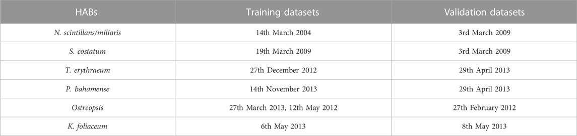
TABLE 1. MODIS datasets (time periods) to train and validate the SVD-model for detecting and delineating different HAB types in the Red Sea.

2.2 In-situ datasets

We examined in-situ datasets from different sampling HAB campaigns. Alkawri et al. (2016a) conducted a field sampling program over the period of June 2012 to September 2013 and reported the occurrence of dinoflagellate P. bahamense and cyanobacteria T. erythraeum in the Al-Hodeidah coastal waters. In addition, several other HAB species including the toxic dinoflagellates K. foliaceum and Protoperidinium quinquecorne have also been identified in the Al-Hodeidah coastal waters during this sampling HAB campaign (Alkawri, 2016; Alkawri et al., 2016b). In-situ studies conducted in the fish landing center of Al-Hodeidah city reported a mixed-species HAB assemblage that was composed of dinoflagellate N. scintillans/miliaris and diatom S. costatum in March 2009 (Alkershi and Menon, 2011). We further utilized in-situ datasets from Catania et al. (2017) who reported the presence of the toxic dinoflagellate Ostreopsis sp. during February 2012, May 2012, and March 2013 off the Thuwal coast (Saudi Arabia). We finally analyzed in-situ datasets from previous studies that reported toxic dinoflagellate P. bahamense blooms and N. scintillans/miliaris in Thuwal and Al Shuqaiq coastal waters (Saudi Arabia) during November 2013 and March 2004, respectively (Mohamed and Mesaad, 2007; Banguera-Hinestroza et al., 2016). These detailed survey datasets included oceanographic measurements such as temperature, salinity, and cell counts, and are documented by different studies (see Supplementary Tables S1, S2) (Alkawri, 2016; Alkawri et al., 2016a; b; Alkershi and Menon, 2011; Catania et al., 2017). Although these are the most comprehensive in-situ datasets on HABs available in the Red Sea, we acknowledge this is still an under-sampled region. The daily spatial matchups between MODIS-Aqua observations and the in-situ measurements were attained by selecting the nearest 1 km pixel (closest longitude and latitude) to the field sampling location.

2.3 Training dataset and SVD approach

A training dataset was established by collecting samples from daily MODIS-Aqua images concurrently collected alongside available in-situ datasets on HABs in the Red Sea (see Supplementary Table S2). The training dataset included measurements of R_rs spectra for the different HAB species that were documented in the basin (Figure 1). A total of 770 samples were collected from HAB-dominated areas in the Red Sea basin for the training dataset. We utilised a median filter with tolerance to remove extreme outliers from the class distributions. The tolerance of the median filter for the training data was determined based on the standard deviation of the distribution. The tolerance (ζ_tol) was used to maintain spectral variation for each HAB class while eliminating extreme outliers from the upper and lower bounds. Thus, the training data for the model can be expressed as

$\mathrm{m}\mathrm{e}\mathrm{d}\left(R_{rs}\right)-{\zeta }_{\mathrm{t}\mathrm{o}\mathrm{l}}\le R_{rs}\le \mathrm{m}\mathrm{e}\mathrm{d}\left(R_{rs}\right)+{\zeta }_{\mathrm{t}\mathrm{o}\mathrm{l}}(1)$

FIGURE 1

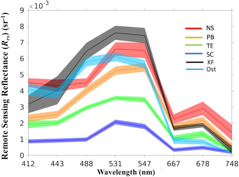
FIGURE 1. MODIS-derived R_rs spectra of N. scintillans/miliaris (NS), P. bahamense (PB), T. erythraeum (TE), S. costatum (SC), K. foliaceum (KF), and Ostreopsis (Ost) blooms in the Red Sea.

By applying the median filter, the number of HAB samples in the training dataset was reduced to 523 samples. For instance, the number of training data was reduced to 241 samples for T. erythraeum, 152 samples for P. bahamense, 49 samples for N. scintillans/miliaris, 40 samples for S. costatum, 21 samples for K. foliaceum, and 20 samples for Ostreopsis. We then developed an algorithm based on the SVD technique for detecting and delineating the species-specific HABs. The steps of the proposed SVD-model for detecting and delineating Red Sea HABs are outlined in Figure 2. The first step was to generate a training data matrix A from the R_rs spectra of these HABs defined as,

$A=\left|\begin{array}{c}{R}_{11}{R}_{12}{R}_{13}\dots .R_{1n}\\ R_{21}{R}_{22}{R}_{23}\dots .R_{2n}\\ R_{31}{R}_{32}{R}_{33}\dots .R_{3n}\\ .....\\ .....\\ .....\\ R_{m1}{R}_{m2}{R}_{m3}\dots .R_{mn}\end{array}\right|(2)$

FIGURE 2

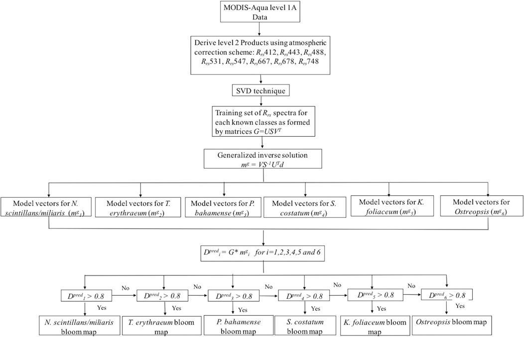
FIGURE 2. Flow diagram of an SVD model for detecting and delineating HABs in the Red Sea.

where A is a MxN matrix, with M and N the MODIS-Aqua pixels and wavelengths, respectively, and R is the R_rs observations of these HAB species. The SVD technique was then used to decompose the training data-matrix A as,

$A=U\Lambda V^T(3)$

where Λ is a diagonal matrix, U and V are the orthogonal matrices (Danaher and O'Mongain, 1992).

In the second step, the generalized inverse model (m^g) was computed based on the SVD as,

$m^g=U^T\Lambda \mathrm{V}{D}^{obs}(4)$

where m^g is a Nx1 vector and D^obs is the data observation vector of size Mx1. If the in-situ sampling pixels denote the presence of HABs, then the element of D^obs is 1, and 0 otherwise.

3 Results and discussion

Based on the SVD analysis, all the reported HABs in the Red Sea were efficiently classified and distinguished as shown in Figure 3. To achieve this, the predicted data values (D^pred_i) were computed for all HABs as Am^g_i of respective species (for i = 1,2,3,4,5, and 6). By specifying a threshold value of 0.8 to the computed D^pred_i values of all classes, the SVD approach was capable of classifying the HAB species in the Red Sea waters. For example, the D^pred₁ and D^pred₂ values of all classes were computed with respect to “m^g₁” and “m^g₂” for N. scintillans/miliaris and T. erythraeum blooms, respectively. By defining a threshold value of 0.8, all N. scintillans/miliaris and T. erythraeum bloom classes were accurately classified (Figures 3A, B). Similarly, all P. bahamense and S. costatum samples were delineated using the same threshold (Figures 3C, D). In Figures 3E, F, K. foliaceum and Ostreopsis samples were also accurately classified using D^pred₅ > 0.8 and D^pred₆ > 0.8, respectively. We then applied the proposed SVD-model to MODIS-Aqua satellite observations and assessed its performance against the standard SOD approach that has been previously implemented for detecting and mapping the Red Sea HABs (Gokul et al., 2019).

FIGURE 3

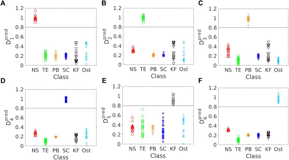
FIGURE 3. Results of the SVD analysis. (A–F) Predicted data Values (D^pred_i) > 0.8 delineate the HAB pixels. NS- N. scintillans/miliaris; TE- T. erythraeum; PB- P. bahamense; SC- S. costatum; KF- K. foliaceum; Ost-Ostreopsis.

We first investigated the daily MODIS-Aqua image on 3^rd March 2009 for detecting the dinoflagellate N. scintillans/miliaris and the diatom S. costatum over the southern Red Sea (SRS) region. In the false color composite (FCC) MODIS image, the dark red features suggested the presence of HABs that were characterized by enhanced reflectance at the red bands (Figures 4A, B). In Figure 4C, an aggregation of elevated Chl-a values (>2 mg m⁻³) was identified in the open and coastal waters of the SRS. It was also observed that the high Chl-a observations appear to coincide spatially with the HABs detected by the SOD approach (Figure 4D). However, the SOD approach is limited for distinguishing some mixed HAB classes such as diatoms with dinoflagellates, as reported in Gokul et al. (2019). In contrast, the SVD-model has the capability of detecting the patterns of these two different HAB species, and distinguishing between them (Figure 4E). The prevailing south-easterly winds seemed to be responsible for transferring these water masses hundreds of kilometers away, while re-distributing the HAB event (>5000 km²) in the open Red Sea waters (Gokul et al., 2020). As shown in Figure 4E, the proposed SVD-model also mapped the large-scale spatial distributions of this mixed-species HAB assemblage over the SRS. The presence of dinoflagellate N. scintillans/miliaris and diatom S. costatum blooms detected by the SVD-model was found to match markedly well with the in-situ observations recorded along the Al-Hodeidah coastal waters during March 2009 (Figures 4E, F).

FIGURE 4

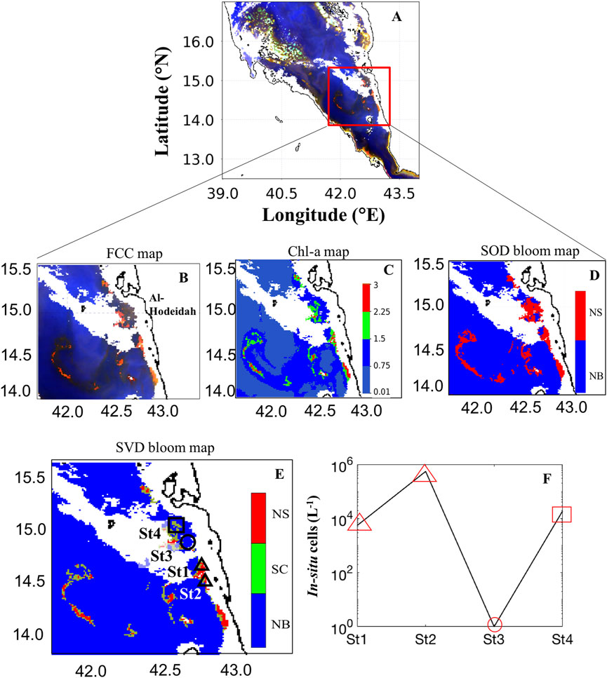
FIGURE 4. Remotely sensing HABs over the southern Red Sea (SRS) on 3^rd March 2009. (A, B) False color composite (FCC) map of the SRS [FCC map is processed using the R_rs measurements at wavelengths of 748, 555, 412 nm]. (C) ABI-derived Chl-a map. (D) Bloom map based on the Second-order derivative technique of Gokul et al. (2019). (E) Bloom map based on the singular value decomposition technique [In (D) and (E) NS- N. scintillans/miliaris; SC- S. costatum; NB- Non-bloom waters. In (E) the black square, triangles and circle indicate in-situ sampling points for the presence of SC, NS and absence of HABs, respectively]. (F) Variations of in-situ cell counts for HABs associated with two different PFTs including dinoflagellate N. scintillans/miliaris observed in the stations “St1” and “St2”, and the diatom S. costatum recorded from the station “St4” in the Yemeni coastal waters, SRS on 3rd March 2009. We note that NS and SC blooms were not detected from the station “St3” along the Al-Hodeidah coast [The SVD-model detection of SC, NS, and absence of HABs were indicated by a red square, triangles and circle, respectively].

Similarly, the daily MODIS image acquired on 29th April 2013 was analyzed for detecting the dinoflagellate P.bahamense and cyanobacteria T. erythraeum blooms in the Al-Hodeidah coastal waters. The spatial coverage of these blooms based on FCC imagery was very low due to the high suspended sediments and bottom reflection along the coast of Al-Hodeidah (bright features in the area outlined with the red box in Figure 5A). This suggests some limitations in the use of the FCC map to identify the water discoloration due to HABs. However, high Chl-a values identified along the coast of Al-Hodeidah and noticeable patches of those elevated Chl-a concentrations were spatially consistent with the presence of HABs, as depicted by bloom map images from the SOD and SVD approaches (Figures 5B–D). In Figure 5D, the SVD-approach was able to detect and delineate the dinoflagellate P.bahamense and cyanobacteria T. erythraeum blooms in the Al-Hodeidah coastal waters. The SVD-model results were in agreement with an in-situ measurement of T. erythraeum, which was collected at the station “St1” in the Al-Hodeidah coastal waters (Figures 5E, F). Besides, the distribution of P.bahamense detected by the SVD-model was found to be consistent with the in-situ observations recorded at the stations “St2” and “St3” in the coastal areas of Al-Hodeida City (SRS) (Figures 5E, F).

FIGURE 5

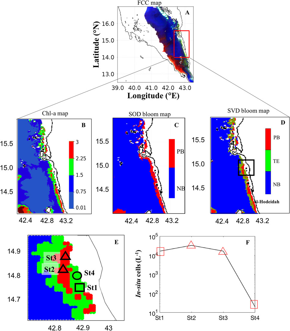
FIGURE 5. Remotely sensing HABs in the Al-Hodeidah coastal waters on 29 April 2013. (A) False color composite (FCC) image [FCC map is processed using the R_rs measurements at wavelengths of 748, 555, 412 nm]. (B) ABI-derived Chl-a map. (C) Bloom map based on the Second-order derivative technique of Gokul et al. (2019). (D, E) Bloom map based on the singular value decomposition technique [In (C) and (D) PB- P. bahamense; TE- T. erythraeum; NB- Non-bloom waters. In (E) the in-situ sampling points of PB, TE, and the absence of HABs are indicated by the black triangles, square and circle, respectively]. (F) Variations of in-situ cell counts for HABs associated with two different PFTs including the cyanobacteria T. erythraeum recorded from the station “St1” and the dinoflagellate P. bahamense recorded from the stations “St2” and “St3” along the Al-Hodeidah coastal waters. We note that no HAB species were observed from the station “St4” along the Al-Hodeidah coast [red triangles and squares denote SVD-model detection of PB and TE, respectively].

Some limitations were also noticed in the SVD-model’s accuracy along the Al-Hodeidah coastal waters in particular at Station “St4” in Figures 5E, F. For instance, during 29th April 2013, the SVD-model falsely identified T. erythraeum blooms at the station "St4" along the Al-Hodeidah coast where the in-situ data indicated the absence of HAB species (Figures 5E, F). Previous studies have suggested that enhanced radiance caused by shallow bathymetry, and certain combinations of CDOM and non-algal particles (such as sediments) could mimic the T. erythraeum blooms reflectance pattern (Subramaniam et al., 1999; Subramaniam et al., 2001; Hu et al., 2010). Under such conditions, satellite ocean color measurements are limited to discriminate T. erythraeum blooms from other non-phytoplankton features (Subramaniam et al., 1999; Subramaniam et al., 2001; Gokul et al., 2019). One way to address this limitation may be to consider additional remotely-sensing datasets such as SST, PAR and wind, which were used to efficiently discriminate T. erythraeum blooms from other highly reflective features in the coastal waters (Subramaniam et al., 1999; Subramaniam et al., 2001; Raitsos et al., 2008).

We finally analyzed the daily MODIS-Aqua image on 29th June 2015 to investigate the HAB species that were associated with different PFT groupings over the south-central Red Sea (SCRS). Gokul et al. (2020) demonstrated that the HABs were detected as large-scale events (>5000 km²) in the SCRS region during summer 2015. In Figure 6A, these large-scale HABs were identified as dark red features in the FCC map, because of enhanced radiance at red bands over the SCRS region. This is consistent with Hu et al. (2005) who suggested that FCC imagery can discriminate the dark features due to high light absorption associated with the presence of phytoplankton biomass (including HABs), from other bright features due to non-algal substances such as bottom reflection and suspended sediments. As evident in Figure 6B, the patches of elevated Chl-a (>2 mg m-3) were identified in the SCRS waters. It concurs with Li et al. (2017) who observed a high Chl-a event on 29^th June 2015 over the SCRS region. Furthermore, the SOD and SVD models were able to map the HAB event that was associated with these elevated Chl-a concentrations over the SCRS region (Figures 6C, D). The SVD approach further has the ability to detect and delineate the HABs associated with the mixed assemblages of three different PFTs including dinoflagellates, cyanobacteria, and diatoms in the open and coastal waters of SCRS during 29th June 2015 (Figure 6D). It is important to note that no in-situ observations were recorded during this HAB event over the SCRS region, although their presence was detected during June 2015 and reported by Gokul et al. (2020).

FIGURE 6

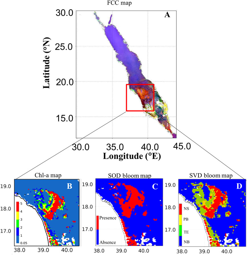
FIGURE 6. Remotely sensing HAB over the south-central Red Sea (SCRS) on 29^th June 2015. (A) False color composite (FCC) image [FCC map is processed using the R_rs measurements at wavelengths of 748, 555, 412 nm]. (B) ABI-derived Chl-a map. (C) Bloom map based on the Second-order derivative technique of Gokul et al. (2019). (D) Bloom map based on the singular value decomposition technique [In (D) NS- N. scintillans/miliaris; SC- S. costatum; TE- T. erythraeum; NB- Non-bloom waters].

We further assessed the overall accuracy of the SVD-model against the SOD-model for detecting and delineating the six different Red Sea HABs (see Supplementary Figures S2, S3 for the SVD and SOD models derived K. foliaceum and Ostreopsis blooms). An error matrix was constructed for each of the two models from the spatial matchups between satellite-derived HAB observations and in-situ measurements (Table 2; Table 3), including the following metrics: producer’s accuracy, overall accuracy, user’s accuracy, and the Kappa coefficient (see footnote “a” and “b” of Tables 2, 3, respectively). Based on the in-situ datasets available for validation (18 samples), we compared the overall accuracy of the SOD and SVD approaches. Our results suggested that the SVD-model has a better agreement with the in-situ datasets with an overall accuracy of 94.4%, compared to 83.3% from the SOD-model. The SOD and SVD approaches were both trained using the shape (curvature) of R_rs spectra across the entire visible wavelengths for detecting and delineating the HAB species associated with different PFT groupings. For instance, the SOD approach was used to assess the R_rs spectral shapes of different HAB species and identify the local troughs and peaks of R_rs across the entire visible region for detecting species-specific Red Sea HABs (Gokul et al., 2019). Although the SOD approach was able to identify the Red Sea HABs from R_rs data, it is limited to distinguishing some mixed HAB species exhibiting similar spectral shapes but varying magnitudes. This is due to the fact that the SOD approach was trained solely on spectral shape information. The success of the present approach could be attributed to the fact that the SVD technique exploits both spectral magnitude and spectral shape information across the entire visible wavelengths to detect and delineate species-specific Red Sea HABs. We also acknowledge a limitation regarding the satellite ocean color observations used in this study. For example, MODIS-Aqua observations over the SRS region in the summer (June-August) are severely limited by the persistent cloud cover, sensor saturation over sand, and sun-glint (Steinmetz et al., 2011; Brewin et al., 2015; Racault et al., 2015; Raitsos et al., 2015; Dreano et al., 2016; Gokul et al., 2020). This limited the ability of the SVD-model to investigate the HABs composed of toxic dinoflagellate P. quinquecorne and cyanobacteria T. erythraeum that were reported by Alkawri et al. (2016a,b) along the Al-Hodeidah coast on 12^th June 2012. In addition, the Red Sea is a severely under-sampled region, despite being substantially impacted by HABs (Mohamed 2018; Gokul et al., 2019; Gokul et al., 2020). Due to the lack of adequate in-situ HAB observations in the Red Sea region, it is difficult to evaluate the proposed SVD model’s ability to map mixed-species HAB assemblages over large spatiotemporal scales in the basin. The availability of greater numbers of regional in-situ measurements in the future would enable further assessment of the capacity of the SVD-model to map multi-species HABs in the Red Sea.

TABLE 2

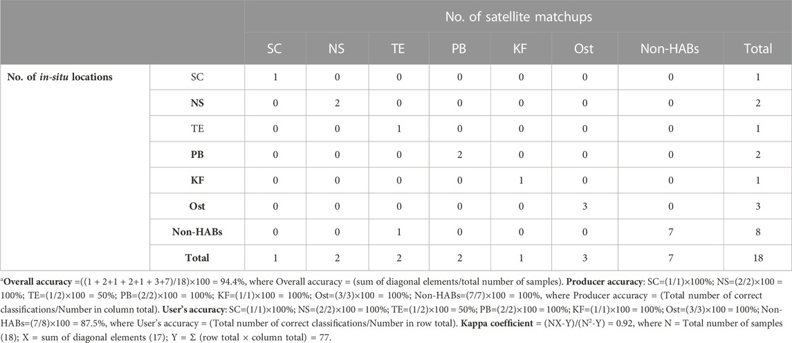
TABLE 2. Accuracy assessment of SVD model for detecting S. costatum (SC), N. scintillans/miliaris (NS), T. erythraeum (TE), P. bahamense (PB), K. foliaceum (KF), and Ostreopsis (Ost) blooms^a.

TABLE 3

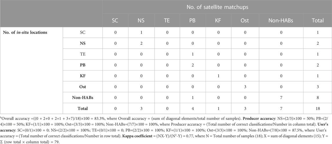
TABLE 3. Accuracy assessment of SOD model for detecting S. costatum (SC), N. scintillans/miliaris (NS), T. erythraeum (TE), P. bahamense (PB), K. foliaceum (KF), and Ostreopsis (Ost) blooms^b.

4 Conclusion

In summary, combining satellite-derived R_rs observations and the SVD technique for detecting and delineating HABs in the Red Sea appears promising. The SVD-model’s performance was validated with the concurrent field observations and further assessed against the SOD-model that was implemented by Gokul et al. (2019) for detecting and mapping the Red Sea HABs. Our results suggested that the SVD model has a better agreement with the available in-situ datasets, in comparison to the SOD-model. We showed that the SVD-model can separate the desired phytoplankton signal from the spectral distributions of different PFTs and produce spatial maps of mixed-species HAB assemblages. We also acknowledge the SVD model’s limitations of falsely detecting Trichodesmium blooms in the shallow coastal waters of the Red Sea, where high bottom reflections and non-algal substances could mimic the reflectance pattern of these blooms. The SVD algorithm’s capacity at detecting and mapping multi-species HABs is currently limited to the Red Sea basin. Consequently, future efforts could focus on including additional training datasets to enhance the model’s ability to detect and monitor these events in other oceans. The SVD model could be further retrained using other multi-spectral satellite sensors such as Sentinel-3 (at a 300 m spatial resolution), to scrutinize its adaptability as a remote sensing tool to investigate mixed-species HAB events at a higher spatial resolution. The SVD model’s versatility in utilizing available satellite remote sensing data makes it suitable for mapping the spatiotemporal distributions of species-specific HABs in the Red Sea. Such information will assist policymakers in implementing integrated management strategies for predicting, mitigating, controlling, and preventing HABs to ensure the economic sustainability of the Red Sea coastal zone.

Data availability statement

The raw data supporting the conclusions of this article will be made available by the authors, without undue reservation.

Author contributions

EG designed the study, analyzed the data, validated the data, and drafted the work. DR, RB, and IH contributed to the writing, reviewing and editing of this manuscript.

Funding

This work was supported by the Office of sponsored Research (OSR) at King Abdullah University of Science and Technology (KAUST) under the virtual Red Sea Initiative (Grant # REP/1/3268-01-01). RB was supported by a UKRI Future Leader Fellowship (MR/V022792/1).

Acknowledgments

We acknowledge the Ocean Biology Processing Group of NASA for distributing the MODIS-Aqua data and developing and supporting SeaDAS software. We thank Abdulsalam Alkawri for providing the in-situ dataset of HABs in the Red Sea. We thank the reviewers for their constructive comments that helped improve an earlier version of the manuscript.

Conflict of interest

The authors declare that the research was conducted in the absence of any commercial or financial relationships that could be construed as a potential conflict of interest.

Publisher’s note

All claims expressed in this article are solely those of the authors and do not necessarily represent those of their affiliated organizations, or those of the publisher, the editors and the reviewers. Any product that may be evaluated in this article, or claim that may be made by its manufacturer, is not guaranteed or endorsed by the publisher.

Supplementary material

The Supplementary Material for this article can be found online at: https://www.frontiersin.org/articles/10.3389/frsen.2023.944615/full#supplementary-material

References

Alkawri, A., Abker, M., Qutaei, E., Alhag, M., Qutaei, N., and Mahdy, S. (2016a). The first recorded bloom of Pyrodinium bahamense var bahamense plate in Yemeni coastal waters off Red Sea, near Al Hodeida City. Turk. J. Fish. Aquat. Sci. 16 (2), 275–282. doi:10.4194/1303-2712-v16_2_07

CrossRef Full Text | Google Scholar

Alkawri, A., Al Areeki, M., and Alsharaby, K. (2016b). The first recorded bloom of Protoperidinium quinquecorne and its link to a massive fish kill in Yemeni coastal waters. Plankton Benthos Res. 11 (2), 75–78. doi:10.3800/pbr.11.75

CrossRef Full Text | Google Scholar

Alkawri, A. (2016). Seasonal variation in composition and abundance of harmful dinoflagellates in Yemeni waters, southern Red Sea. Mar. Pollut. Bull. 112 (1-2), 225–234. doi:10.1016/j.marpolbul.2016.08.015

PubMed Abstract | CrossRef Full Text | Google Scholar

Alkershi, A., and Menon, N. (2011). Phytoplankton in polluted waters of the Red Sea coast of Yemen. J. Mar. Biol. Assoc. India 53 (2), 161–166. doi:10.6024/jmbai.2011.53.2.01630-01

CrossRef Full Text | Google Scholar

Alvain, S., Moulin, C., Dandonneau, Y., and Bréon, F. M. (2005). Remote sensing of phytoplankton groups in case 1 waters from global SeaWiFS imagery. Deep-Sea Res. I Oceanogr. Res. Pap. 52 (11), 1989–2004. doi:10.1016/j.dsr.2005.06.015

CrossRef Full Text | Google Scholar

Anderson, D. M. (2009). Approaches to monitoring, control and management of harmful algal blooms (HABs). Ocean. Coast. Manag. 52 (7), 342–347. doi:10.1016/j.ocecoaman.2009.04.006

PubMed Abstract | CrossRef Full Text | Google Scholar

Anderson, D. M., Cembella, A. D., and Hallegraeff, G. M. (2012). Progress in understanding harmful algal blooms: Paradigm shifts and new technologies for research, monitoring, and management. Annu. Rev. Mar. Sci. 4, 143–176. doi:10.1146/annurev-marine-120308-081121

PubMed Abstract | CrossRef Full Text | Google Scholar

Anderson, D. M., Glibert, P. M., and Burkholder, J. M. (2002). Harmful algal blooms and eutrophication: Nutrient sources, composition, and consequences. Estuaries 25 (4), 704–726. doi:10.1007/bf02804901

CrossRef Full Text | Google Scholar

Banguera-Hinestroza, E., Eikrem, W., Mansour, H., Solberg, I., Curdia, J., Holtermann, K., et al. (2016). Seasonality and toxin production of Pyrodinium bahamense in a Red Sea lagoon. Harmful algae 55, 163–171. doi:10.1016/j.hal.2016.03.002

PubMed Abstract | CrossRef Full Text | Google Scholar

Berdalet, E., Fleming, L. E., Gowen, R., Davidson, K., Hess, P., Backer, L. C., et al. (2016). Marine harmful algal blooms, human health and wellbeing: Challenges and opportunities in the 21st century. J. Mar. Biol. 96 (1), 61–91. doi:10.1017/s0025315415001733

CrossRef Full Text | Google Scholar

Bracher, A., Vountas, M., Dinter, T., Burrows, J. P., Röttgers, R., and Peeken, I. (2009). Quantitative observation of cyanobacteria and diatoms from space using PhytoDOAS on SCIAMACHY data. Biogeosciences 6 (5), 751–764. doi:10.5194/bg-6-751-2009

CrossRef Full Text | Google Scholar

Brewin, R. J., Raitsos, D. E., Dall'Olmo, G., Zarokanellos, N., Jackson, T., Racault, M. F., et al. (2015). Regional ocean-colour chlorophyll algorithms for the Red Sea. Remote Sens. Environ. 165, 64–85. doi:10.1016/j.rse.2015.04.024

CrossRef Full Text | Google Scholar

Brewin, R. J., Raitsos, D. E., Pradhan, Y., and Hoteit, I. (2013). Comparison of chlorophyll in the Red Sea derived from MODIS-Aqua and in vivo fluorescence. Remote Sens. Environ. 136, 218–224. doi:10.1016/j.rse.2013.04.018

CrossRef Full Text | Google Scholar

Catania, D., Richlen, M. L., Mak, Y. L., Morton, S. L., Laban, E. H., Xu, Y., et al. (2017). The prevalence of benthic dinoflagellates associated with ciguatera fish poisoning in the central Red Sea. Harmful algae 68, 206–216. doi:10.1016/j.hal.2017.08.005

PubMed Abstract | CrossRef Full Text | Google Scholar

Correa-Ramirez, M., Morales, C. E., Letelier, R., Anabalón, V., and Hormazabal, S. (2018). Improving the remote sensing retrieval of phytoplankton functional types (PFT) using empirical orthogonal functions: A case study in a coastal upwelling region. Remote Sens. 10 (4), 498. doi:10.3390/rs10040498

CrossRef Full Text | Google Scholar

Danaher, S., and O'Mongain, E. (1992). Singular value decomposition in multispectral radiometry. Int. J. Remote Sens. 13 (9), 1771–1777. doi:10.1080/01431169208904226

CrossRef Full Text | Google Scholar

Devred, E., Martin, J., Sathyendranath, S., Stuart, V., Horne, E., Platt, T., et al. (2018). Development of a conceptual warning system for toxic levels of Alexandrium fundyense in the Bay of Fundy based on remote sensing data. Remote Sens. Environ. 211, 413–424. doi:10.1016/j.rse.2018.04.022

CrossRef Full Text | Google Scholar

Dreano, D., Raitsos, D. E., Gittings, J., Krokos, G., and Hoteit, I. (2016). The Gulf of Aden intermediate water intrusion regulates the southern Red Sea summer phytoplankton blooms. PLoS one 11 (12), e0168440. doi:10.1371/journal.pone.0168440

PubMed Abstract | CrossRef Full Text | Google Scholar

Dwivedi, R., Rafeeq, M., Smitha, B. R., Padmakumar, K. B., Thomas, L. C., Sanjeevan, V. N., et al. (2015). Species identification of mixed algal bloom in the Northern Arabian Sea using remote sensing techniques. Environ. Monit. Assess. 187 (2), 51–11. doi:10.1007/s10661-015-4291-2

PubMed Abstract | CrossRef Full Text | Google Scholar

Gittings, J. A., Raitsos, D. E., Krokos, G., and Hoteit, I. (2018). Impacts of warming on phytoplankton abundance and phenology in a typical tropical marine ecosystem. Sci. Rep. 8 (1), 1–12. doi:10.1038/s41598-018-20560-5

PubMed Abstract | CrossRef Full Text | Google Scholar

Gokul, E. A., Raitsos, D. E., Gittings, J. A., Alkawri, A., and Hoteit, I. (2019). Remotely sensing harmful algal blooms in the Red Sea. PLoS one 14 (4), e0215463. doi:10.1371/journal.pone.0215463

PubMed Abstract | CrossRef Full Text | Google Scholar

Gokul, E. A., Raitsos, D. E., Gittings, J. A., and Hoteit, I. (2020). Developing an atlas of harmful algal blooms in the Red Sea: Linkages to local aquaculture. Remote Sens. 12 (22), 3695. doi:10.3390/rs12223695

CrossRef Full Text | Google Scholar

Gokul, E. A., and Shanmugam, P. (2016). An optical system for detecting and describing major algal blooms in coastal and oceanic waters around India. J. Geophys. Res. Oceans. 121 (6), 4097–4127. doi:10.1002/2015jc011604

CrossRef Full Text | Google Scholar

Hu, C., Cannizzaro, J., Carder, K. L., Muller-Karger, F. E., and Hardy, R. (2010). Remote detection of Trichodesmium blooms in optically complex coastal waters: Examples with MODIS full-spectral data. Remote Sens. Environ. 114 (9), 2048–2058. doi:10.1016/j.rse.2010.04.011

CrossRef Full Text | Google Scholar

Hu, C., Muller-Karger, F. E., Taylor, C. J., Carder, K. L., Kelble, C., Johns, E., et al. (2005). Red tide detection and tracing using MODIS fluorescence data: A regional example in SW Florida coastal waters. Remote Sens. Environ. 97 (3), 311–321. doi:10.1016/j.rse.2005.05.013

CrossRef Full Text | Google Scholar

Li, W., El-Askary, H., Manikandan, K. P., Qurban, M. A., Garay, M. J., and Kalashnikova, O. V. (2017). Synergistic use of remote sensing and modeling to assess an anomalously high chlorophyll-a event during summer 2015 in the South Central Red Sea. Remote Sens. 9 (8), 778. doi:10.3390/rs9080778

CrossRef Full Text | Google Scholar

Liu, Y., Boss, E., Chase, A., Xi, H., Zhang, X., Röttgers, R., et al. (2019). Retrieval of phytoplankton pigments from underway spectrophotometry in the Fram Strait. Remote Sens. 11 (3), 318. doi:10.3390/rs11030318

CrossRef Full Text | Google Scholar

Mohamed, Z. A., and Mesaad, I. (2007). First report on Noctiluca scintillans blooms in the Red Sea off the coasts of Saudi Arabia: Consequences of eutrophication. Oceanologia 49 (3), 337–351. doi:10.5697/oc.53-1.121

CrossRef Full Text | Google Scholar

Mohamed, Z. A. (2018). Potentially harmful microalgae and algal blooms in the Red Sea: Current knowledge and research needs. Mar. Environ. Res. 140, 234–242. doi:10.1016/j.marenvres.2018.06.019

PubMed Abstract | CrossRef Full Text | Google Scholar

Moisan, T. A., Rufty, K. M., Moisan, J. R., and Linkswiler, M. A. (2017). Satellite observations of phytoplankton functional type spatial distributions, phenology, diversity, and ecotones. Front. Mar. Sci. 4, 189. doi:10.3389/fmars.2017.00189

CrossRef Full Text | Google Scholar

Racault, M. F., Raitsos, D. E., Berumen, M. L., Brewin, R. J., Platt, T., Sathyendranath, S., et al. (2015). Phytoplankton phenology indices in coral reef ecosystems: Application to ocean-color observations in the Red Sea. Remote Sens. Environ. 160, 222–234. doi:10.1016/j.rse.2015.01.019

CrossRef Full Text | Google Scholar

Raitsos, D. E., Lavender, S. J., Maravelias, C. D., Haralabous, J., Richardson, A. J., and Reid, P. C. (2008). Identifying four phytoplankton functional types from space: An ecological approach. Limnol. Oceanogr. 53 (2), 605–613. doi:10.4319/lo.2008.53.2.0605

CrossRef Full Text | Google Scholar

Raitsos, D. E., Pradhan, Y., Brewin, R. J., Stenchikov, G., and Hoteit, I. (2013). Remote sensing the phytoplankton seasonal succession of the Red Sea. PLoS one 8 (6), e64909. doi:10.1371/journal.pone.0064909

PubMed Abstract | CrossRef Full Text | Google Scholar

Raitsos, D. E., Yi, X., Platt, T., Racault, M. F., Brewin, R. J., Pradhan, Y., et al. (2015). Monsoon oscillations regulate fertility of the Red Sea. Geophys. Res. Lett. 42 (3), 855–862. doi:10.1002/2014gl062882

CrossRef Full Text | Google Scholar

Sathyendranath, S., Aiken, J., Alvain, S., Barlow, R., Bouman, H., Bracher, A., et al. (2014). Phytoplankton functional types from space. Rep. Int. Ocean-Colour Coord. Group (IOCCG) 15, 1–156. doi:10.25607/OBP-106

CrossRef Full Text | Google Scholar

Shen, L., Xu, H., and Guo, X. (2012). Satellite remote sensing of harmful algal blooms (HABs) and a potential synthesized framework. J. Sens. 12 (6), 7778–7803. doi:10.3390/s120607778

PubMed Abstract | CrossRef Full Text | Google Scholar

Singh, R. K., and Shanmugam, P. (2014). A novel method for estimation of aerosol radiance and its extrapolation in the atmospheric correction of satellite data over optically complex oceanic waters. Remote Sens. Environ. 142, 188–206. doi:10.1016/j.rse.2013.12.001

CrossRef Full Text | Google Scholar

Steinmetz, F., Deschamps, P. Y., and Ramon, D. (2011). Atmospheric correction in presence of sun glint: Application to MERIS. Opt. Express. 19 (10), 9783–9800. doi:10.1364/oe.19.009783

PubMed Abstract | CrossRef Full Text | Google Scholar

Stumpf, R. P., and Tomlinson, M. C. (2007). “Remote sensing of harmful algal blooms,” in Remote sensing of coastal aquatic environments (Dordrecht: Springer), 7, 277–296. doi:10.1007/978-1-4020-3100-7_12

CrossRef Full Text | Google Scholar

Subramaniam, A., Brown, C. W., Hood, R. R., Carpenter, E. J., and Capone, D. G. (2001). Detecting Trichodesmium blooms in SeaWiFS imagery. Deep Sea Res. Part II Top. Stud. Oceanogr. 49 (1-3), 107–121. doi:10.1016/s0967-0645(01)00096-0

CrossRef Full Text | Google Scholar

Subramaniam, A., Carpenter, E. J., and Falkowski, P. G. (1999). Bio-optical properties of the marine diazotrophic cyanobacteria Trichodesmium spp. II. A reflectance model for remote sensing. Limnol. Oceanogr. 44 (3), 618–627. doi:10.4319/lo.1999.44.3.0618

CrossRef Full Text | Google Scholar

Zhao, J., Temimi, M., and Ghedira, H. (2015). Characterization of harmful algal blooms (HABs) in the Arabian Gulf and the Sea of Oman using MERIS fluorescence data. ISPRS J. Photogramm. Remote Sens. 101, 125–136. doi:10.1016/j.isprsjprs.2014.12.010

CrossRef Full Text | Google Scholar