Observation and modeling of an unusual spatiotemporal pattern in bioacoustic chorusing

This paper describes an unusual underwater biological chorus recorded in the Southern California Bight and presents a numerical modeling approach that replicates aspects of the chorus. During one experiment, the evolution of the directionality of the chorusing region over time is suggestive of “The Wave”, the human waves performed by fans periodically standing and sitting in sports stadia around the world; here, the region of chorusing periodically propagated upcoast over 20 km of coastline at nearly 1.5 km/s. The chorus occurs predominantly at night in spring and summer, mostly in very shallow waters near the coast. It increases the underwater sound field levels within chorusing regions by 20–30 dB in the 50 Hz to 1 kHz frequency band. The chorus is composed of three parts; 1) a “sunset chorus” which is a 20-to-30 min continuous roar around sunset with received spectral levels up to 100 dB re 1 μPa²/Hz, 2) a “sunrise chorus” of lower level than the sunset chorus, and 3) an all-night-long cycling chorus. The cycling portion is made up of 15-to-20 s periods of higher received spectral levels (up to 90 dB re 1 μPa²/Hz within the chorusing region) each followed by a 10-to-20 s lull in which the spectral levels drop by 4–10 dB. This alternating pattern repeats every 30–40 s throughout the night. The numerical modeling approach is based on the physics of excitable media. A cellular automaton is used to model the two-dimensional spatial grid occupied by the calling animals (units), with each unit being either in the “resting”, “excitable”, or “active (calling)" state at each time step. Transition from resting to excitable and from active back to resting occurs automatically after a fixed period of time in the present state, whereas the probability of transitioning from excitable to active is determined not only by the elapsed time since entering the excitable state, but also by the received sound level at the unit location, creating a non-linear acoustics-based coupling between units. With appropriate inputs, many determined from measurements of the chorus properties and the individual animal calls themselves, simulations with the model can replicate the cycling levels in the night-long chorus, the continuous din of the sunset chorus, and (once properly initialized) the periodic upcoast evolution of the chorusing region (“The Wave”). When noise from a transiting ship is included in the simulations, the spatiotemporal characteristics of the chorus change appreciably, in ways similar to changes observed during the experiment.

1 Introduction

The underwater sound from biological choruses, in which a significant number of individuals collectively participate in a calling behavior, can be a dominant component of naturally occurring sound in the ocean (e.g., Fish, 1964; Cato, 1978; Rountree et al., 2002; National Research Council, 2003). Numerous studies of choruses have appeared in the literature, typically focusing on their temporal (and temporal frequency) properties. The spatial dependence and directional distribution of biological choruses have received less attention, primarily because of the expense and difficulty in deploying large-aperture, multi-element, time-synchronized arrays in the ocean. Such challenges often preclude use of these advanced sensor systems for bioacoustics-specific studies. However, arrays typically are deployed for other types of ocean acoustics research, and sounds of biological origin almost always are recorded as part of the underwater soundscape. The results presented in this paper take advantage of such opportunistic recordings.

Since underwater sound is a critical aspect of the ocean environment for marine animals, passive acoustic recordings provide important information on marine habitats. In particular, biological choruses have been associated with spawning activity and reproduction (e.g., Winn, 1964; Rountree et al., 2002; Rowell et al., 2020). Conversely, because biological choruses can be a significant part of the ocean background sound field, knowledge of their characteristics is important for assessing sonar system performance.

A biological chorusing behavior with unusual temporal and spatial properties has been observed in nighttime underwater acoustic array recordings off the Southern California coast, as reported previously (D’Spain et al., 1997; D’Spain et al., 2013). These choruses were first described in the gray literature by scientists from the Navy Electronics Laboratory in San Diego (Wenz, 1964; Clapp, 1966). In this paper, the focus is on the spatiotemporal properties of the chorus. During one measurement period, the chorus displayed characteristics reminiscent of “The Wave” performed by spectators at sporting events worldwide (Farkas et al., 2002).

Employing the same philosophy behind the numerical modeling approach in Farkas et al., 2002, the numerical models developed herein to predict the character of chorusing are based on the physics of excitable media. Excitable media are spatially distributed systems far from thermodynamic equilibrium that have the ability to propagate signals without damping. Interaction between units in the medium is nonlinear in nature. Excitable media are found in a wide variety of scientific fields including medicine, biology, chemistry, seismology, human social systems, climate science, physics, electronics, and forestry (see Winfree, 2001 for a review). Studies of excitable media follow one of two approaches; those that use numerical modeling techniques, particularly ones in the category of cellular automata (e.g., Greenberg and Hastings, 1978), and those that are analytically based on partial differential equations (Murray and Murray, 1993). Although the former approach can have problems reproducing some of the features observed in excitable media (Gerhardt, M., H. Schuster, and J. J. Tyson, 1990), methods have been developed to overcome these shortfalls. More recently, it has been shown that the use of stochastic, rather than deterministic, rules to govern the transition between some of the states (as done in the modeling in this paper; see Sect. 2.2) avoids these earlier problems in a natural, computationally efficient way (Szakály et al., 2007). The major benefit of numerical approaches is that the derivation of the relevant differential equation in many systems can be difficult, particularly those involving higher order biological systems.

The objective of this paper is to describe the temporal and spatial characteristics of an underwater biological chorus recorded off the southern California coast and to develop a stochastic numerical simulation approach based on a cellular automaton model for the physics of excitable media that replicates many of the chorus features.

2 Materials and methods

The underwater acoustic array data presented in this paper were collected in a series of ocean acoustics experiments sponsored by the Office of Naval Research in the coastal waters of Southern California. The “SWellEx-1” and “SWellEx-3” experiments were conducted during the summer months in 1993 and 1994, respectively, 15 km west-southwest of the mouth to San Diego Harbor (re the upper map in Figure 1). The “ABM-95” deployment occurred in the springtime of 1995 in 20-m-deep water 3.5 km off the coast of Marine Corps Base Camp Pendleton in northern San Diego County, 75 km north-northwest of the SWellEx site. The lower map in Figure 1 shows the ABM-95 site with reference to the SWellEx site, along with the location of the San Onofre Nuclear Generating Station (SONGS), an additional 12 km to the north-northwest of ABM-95. The bycatch from the salt-water intake pipes at SONGS provides an indication of the species and numbers of individual animals in the coastal environment (Allen et al., 2003; Miller et al., 2011) prior to decommissioning of the power plant in 2013. Included in these intake data are significant numbers of known soniferous fish species (see Discussion). The underwater acoustic recordings in all experiments were made by large aperture, multi-element (order 25–100 hydrophones) arrays that provide high resolution estimates of the directionality of the ocean sound field. The primary focus of this paper is on the data collected in SWellEx-1 by a two-dimensional (2D) horizontal bottom-mounted array. It was comprised of 28 functioning hydrophones elements with spatial aperture of about 60 m in both the north-south and east-west directions. Plots of the array element positions and the array beam pattern using conventional beamforming (equivalent to the array plane wave response) are shown in Figure 2. A variety of beamforming techniques were used to determine the azimuth of arrival of sounds up to the cutoff frequency of the array of nearly 1 kHz (see the next subsection). Whereas data from a single array element collected in SWellEx-3 and ABM-95 are presented in this paper, all beamforming results presented herein were obtained from this 2D horizontal array.

Figure 1

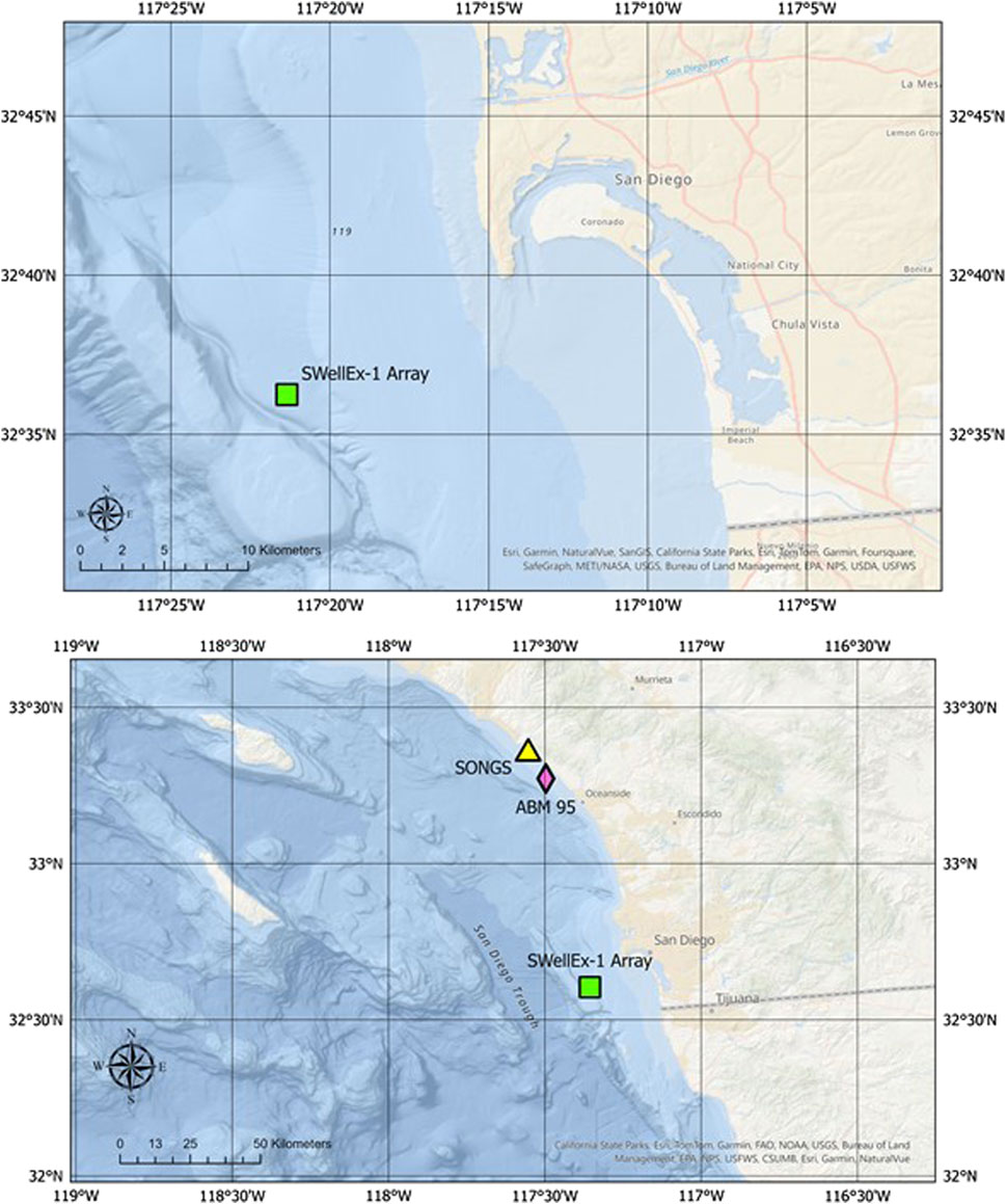
Figure 1. Maps of the offshore region west of San Diego County. The upper map shows the location of the 2-dimensional (2D) horizontal planar array in the SWellEx-1 experiment whose data are used to determine the azimuths of the biological choruses discussed in this paper. The Point Loma peninsula and the entrance to San Diego harbor, just east of the southern tip of Point Loma, are located in the upper center of the map. The lower map is plotted on a larger spatial scale to illustrate the ABM-95 and SONGS positions with respect to SWellEx-1.

Figure 2

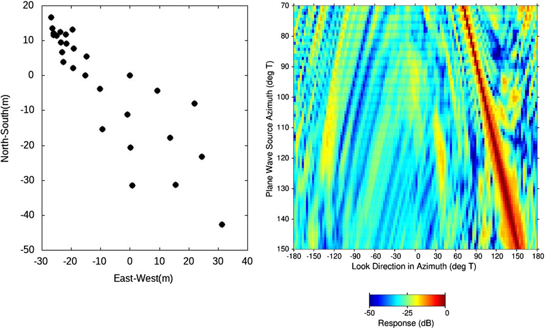
Figure 2. The north-south (vertical axis) and east-west (horizontal positions the 2D horizontal planar array in SWellEx-1 (left plot) and the array beam pattern in azimuth (right-hand plot).

2.1 Array processing

White-noise-constrained adaptive plane wave beamforming (Cox, Zeskind, and Owen, 1987; Gramann, 1992) was used with the data from the 2D bottom-mounted array in SWellEx-1 to analyze the azimuthal directionality of the chorusing sounds. Application of white-noise constrained (WNC) beamforming methods to bioacoustic choruses has been discussed previously (D’Spain and Batchelor, 2006). In summary, the array complex weight vector, $\underset{\sim }{\mathrm{w}},$ at a given frequency in WNC plane wave beamforming is equal to

$\underset{\sim }{\mathrm{w}}=\raisebox{1ex}{${\left(\left[S\right]+e\left[I\right]\right)}^{-1}\underset{\sim }{d}$}\!\left/ \!\raisebox{-1ex}{$\left(\underset{\sim }{d}{\hspace{0.17em}}^H{\left(\left[S\right]+e\left[I\right]\right)}^{-1}\underset{\sim }{\left.d\right)}\right.$}\right.$

where the beamformer output magnitude squared, $S_B$, is

$S_B=\underset{\sim }{\mathrm{w}}{\hspace{0.17em}}^H\left[S\right]\underset{\sim }{\mathrm{w}}$

The quantity $\left[S\right]$ at each circular frequency $\omega$ is the data cross-spectral density matrix (CSDM). (The dependence of the quantities above on the circular frequency has been suppressed for clarity). The CSDM is formed by incoherently averaging (signified by “< … >”) the outer product of the vectors $\underset{\sim }{p}\left(\omega \right)$ containing the complex pressure at frequency $\omega$ across all array elements obtained from the fast-Fourier-transformed estimates (snapshots), i.e., $\left[S\left(\omega \right)\right]=<\underset{\sim }{p}\left(\omega \right)\underset{\sim }{p}{\hspace{0.17em}}^H\left(\omega \right)>$. The quantity $\left[I\right]$ is the identity matrix, $\underset{\sim }{d}$ is the look direction vector normalized so that $\underset{\sim }{d}{\hspace{0.17em}}^H\underset{\sim }{d}$ equals the number of array elements $N,$ and the superscript H represents the Hermitian operator. The scalar $e$, which is added to the diagonal of $\left[S\right]$ before the inverse is taken, is set to constrain the magnitude of the weight vector $\underset{\sim }{\mathrm{w}}$. The name “white noise constraint” comes from fact that the white noise gain of the beamformer at frequency $\omega$ equals $\raisebox{1ex}{$1$}\!\left/ \!\raisebox{-1ex}{$\underset{\sim }{\mathrm{w}}{\hspace{0.17em}}^H\underset{\sim }{\mathrm{w}}$}\right.$. For $e=0$ in the expression for the WNC weight vector above, the beamformer is equivalent to the minimum variance distortionless response processor (Capon, 1969), whereas ignoring $\left[S\right]$ yields the conventional beamformer, $\underset{\sim }{\mathrm{w}}=\raisebox{1ex}{$\underset{\sim }{d}$}\!\left/ \!\raisebox{-1ex}{$\underset{\sim }{d}{\hspace{0.17em}}^H\underset{\sim }{d}$}\right.=\raisebox{1ex}{$\underset{\sim }{d}$}\!\left/ \!\raisebox{-1ex}{$N$}\right.$. In effect, the input beamformer constraint value allows the beamformer to be adjusted between purely conventional beamforming, which is robust but does not provide the finest-achievable spatial resolution nor protection from interfering noise sources at other azimuths, and minimum-variance distortionless response adaptive beamforming, which provides fine spatial resolution and cancellation of interfering noise sources but is not robust. Tests conducted with data collected during transmissions by a broadband source at known direction indicated the most effective constraint value was 9–10 dB. This value yields a beamformer about 5 dB more adaptive than conventional beamforming which has a constraint value in this case of 14.5 dB (equal to $10*\log 28$, where $N=28$ is the number of array elements). These beamformers operate in the frequency domain so the parameters that go into the estimation of the CSDM at each frequency are important considerations. Here, fast-Fourier transform lengths of 1,024 samples (for a frequency resolution of 1.9 Hz at the array element sampling frequency of 1979 samples/sec) were used with 50% overlap in the time series segments, to obtain a total of 30 snapshots that were incoherently averaged to obtain the CSDM estimate.

2.2 Numerical modeling of the choruses based on excitable media

In the numerical models developed in this study, the individual bioacoustic sources (units) are assumed to transition in order between one of three states; 1) resting, to 2) excitable, to 3) active (calling). The approach roughly follows the outline presented in Sect. 5.2 of Lindner et al., 2004. At each time step in a simulation, a set of pre-defined rules are used to determine whether or not each of the units remains in its present state or transitions to the next state. Some of the rules used in this modeling effort are stochastic in nature and the probability of transitioning from one state to the next is determined partly by the properties of the individual units themselves (i.e., no coupling between units) and partly by the state of the surrounding units. The coupling between units is determined by the character of individual calls, the propagation of sound, and the assumed sensitivity of the individuals to received sound levels.

The components of the numerical models are the spatial distribution of animals, the set of rules for transitioning from one state to the next, the properties of the individuals that determine the state-transition probabilities, the character of any external noise or discrete sources that can affect the animals, and the acoustic propagation model. Each of these components will be discussed in turn.

The spatial distribution of units is defined over a rectangular-shaped, 2-dimensional spatial domain that is specified by length $L_x$ and width $L_y$. It is gridded with a uniform spacing in the length and width directions of $dx$ and $dy$, respectively. For the results presented in this paper, the along-coast dimension (length) is set to 20 km, the offshore dimension (width) to 1 km, and the grid spacing is 2 m in both dimensions. The models require a spatial density of units (i.e., number of units per square km), ${\rho }_s$, as input which then is used to calculate the probability, $\mathrm{Pr}\left(unit\right)$), of a unit occupying a given grid point $\left(m,n\right)$ located at $\left(m\bullet dx,n\bullet dy\right)$. A uniform probability distribution initially is employed so that the probability of a unit being located at a given grid point equals the total number of units in the whole rectangular area, ${\rho }_s\bullet L_x\bullet L_y$, divided by the total number of grid points in the area, $\raisebox{1ex}{$\left(L_x\bullet L_y\right)$}\!\left/ \!\raisebox{-1ex}{$\left(dx\cdot dy\right)$}\right.$, so that

$\mathrm{Pr}\left(unit\right)={\rho }_s\bullet dx\bullet dy(1)$

Once the total number and locations of the individuals in the 2D domain are determined by random selection from the uniform probability distribution, they remain fixed in space over the period of the simulation.

Since each of the three states that a unit can be in occur in a given sequence in time, from resting to excitable to active, then three transition probabilities must be specified. The probability of transitioning from resting to excitable and from active to resting are set equal to 1 after specified time delays, and equal to 0 prior to those times. Specifically, an individual calling unit remains in the resting state for a duration ${\tau }_{rest}$ before it automatically becomes excitable. Also, once a given unit becomes active, it calls for specific period of time, ${\tau }_{call}$, and then enters the resting state. That is, the probability density functions for these two transitions are modeled as:

$pdf\left(call\to rest,t\right)=\delta \left(t-\left(t_{call}+{\tau }_{call}\right)\right)(2)$

$pdf\left(rest\to excitable,t\right)=\delta \left(t-\left(t_{rest}+{\tau }_{rest}\right)\right)(3)$

where $\delta$ is the Dirac delta function, $t_{call}$ and $t_{rest}$ are the most recent times at which the unit entered the calling and resting states, respectively, and ${\tau }_{call}$ and ${\tau }_{rest}$ are the fixed time periods of remaining in the calling and resting states, respectively. Therefore, all the stochastic variability in the modeling occurs in a) the spatial distribution of individuals, b) the initial state of each unit at the start of a simulation, and c) the transition from the excitable to active state. This transition probability is determined by a combination of two conditions, 1) the time duration since the unit most recently entered the excitable state, and 2) the level of received sound in a frequency band. Whereas the former condition involves no coupling between units, the latter represents a nonlinear dependence of the transition probability on the states of the surrounding units as well as on the environment.

One modeling approach for this transition probability is to generalize the simple 1-dimensional Poisson process, a statistical model for the random occurrence of events in time (Breiman, 1969). For a Poisson process, the probability distribution for the time interval between events is the exponential distribution. Therefore, the probability density function for the transition from excitable to calling is:

$pdf\left(excitable\to call,t\right)=\gamma \bullet \exp \left(-\gamma \bullet \left(t-t_{excite}\right)\right)(4)$

Here, $\gamma$ is the rate of starting to call when in the excitable state and $t_{excite}$ is the time when the unit most recently entered into the excitable state from the resting state. A starting point in the modeling is to assume this rate of starting to call is constant over time. Therefore, the probability of starting to call at time $t$ is the cumulative distribution of this probability density function, i.e.,

$\mathrm{Pr}\left(excitable\to call,t\right)=1-\exp \left(-\gamma \bullet \left(t-t_{excite}\right)\right)(5)$

If, in addition to assuming the rate is time-independent, it is also assumed the individuals act independently of one another, then a statistical analysis of the system is simple—the mean time, $\mu$, for a unit to complete one cycle through all three states is:

$\mu =\frac{1}{\gamma }+{\tau }_{call}+{\tau }_{rest}(6)$

and the variance, ${\sigma }^2$, of these full-cycle times is:

${\sigma }^2=\frac{1}{{\gamma }^2}(7)$

The system becomes less stochastic and more deterministic as the rate of starting to call, $\gamma$, increases. It also contains a deterministic time delay of ${\tau }_{call}+{\tau }_{rest}$.

As mentioned above, the interaction between units in an excitable medium is nonlinear in nature and the modeling approach used here incorporates this nonlinear interaction by making the rate of starting to call a function of the received sound level at each unit. Specifically, if $RL$ represents the received level at a given unit, then the rate of starting to call as a function of RL is taken as

$\gamma \left(RL\right)\equiv \overline{\gamma }\cdot \left[1+\frac{∆\gamma }{\overline{\gamma }\pi }\mathrm{atan}\left(\frac{RL-R{L}_{tran}}{{\sigma }_{RL}}\right)\right](8)$

where $\overline{\gamma }\equiv \left({\gamma }_{\mathit{max}}+{\gamma }_{\mathit{min}}\right)/2$ and $∆\gamma \equiv {\gamma }_{\mathit{max}}-{\gamma }_{\mathit{min}}$. From this equation, the rate of starting to call equals ${\gamma }_{\mathit{min}}$ at very small values of RL compared to $R{L}_{tran}$ whereas it is ${\gamma }_{\mathit{max}}$ at very large levels. The quantity $R{L}_{tran}$ is the “transition” received sound level at which the arctangent function is most sensitive (i.e., increases/decreases the greatest amount) to changes in received level. At this point, $\gamma \left(R{L}_{tran}\right)=\overline{\gamma }$ and

$\frac{\partial \left[\gamma \left(RL\right)\right]}{\partial RL}\left(R{L}_{tran}\right)=\frac{∆\gamma }{\pi \cdot {\sigma }_{RL}}(9)$

As this equation shows, the parameter ${\sigma }_{RL}$ controls the rate of change in $\gamma$ around $R{L}_{tran}$; small values of ${\sigma }_{RL}$ result in rapid/steep changes and large values lead to gradual changes.

Therefore, the state transition probabilities are determined by properties of the individual bioacoustic units, ${\tau }_{call}:$ duration of calling, ${\tau }_{rest}:$ duration of resting, $R{L}_{tran}:$ level of received sound where the transition probability from excitable to calling is most sensitive to changes in received level, and ${\sigma }_{RL}:$ the “coupling” parameter (Linder et al., 2004) controlling the rate of change in $\gamma .$ In addition to these four quantities, an additional property is the source level of calling, $S{L}_{call}$. The values of ${\gamma }_{\mathit{min}}$ and ${\gamma }_{\mathit{max}}$ are determined by ${\tau }_{call}$ and ${\tau }_{rest}$ and are set so that the mean time, $\mu$, for a unit to complete one cycle can vary from purely stochastic, ${\left({\gamma }_{\mathit{min}}\right)}^{-1}\gg {\tau }_{call}+{\tau }_{rest}$, to purely deterministic, ${\left({\gamma }_{\mathit{max}}\right)}^{-1}\ll {\tau }_{call}+{\tau }_{rest}$. Any of these input properties could be readily randomized across the units in the numerical modeling rather than being assigned fixed values. However, the statistical distributions of only two of the five input parameters, ${\tau }_{call}$ (re Figure 7) and $S{L}_{call}$ were determined from the experimental data. Therefore, a full evaluation of the effects of this randomization is beyond the scope of the paper.

Once the number and locations on the grid of the units have been randomly chosen, the initial state of each unit at the start of the simulation must be defined. In addition, the location, source level, and time interval of transmission of any external sources of sound also must be specified in the model input.

Finally, an acoustic propagation model is used to calculate the received sound level at each unit location at each time step. For the modeling results presented in this paper, the environment is taken as a homogeneous water column of depth 20 m and sound speed 1,500 m/sec. Transmission loss (TL) is calculated with a semi-empirical model developed from fitting physics-based terms in the sonar equation with measured at-sea data from numerous experiments in shallow water (Marsh and Schulkin, 1962). Defining a “skip” or bounce distance, $H,$ in units of Kyds as $H\equiv \sqrt{\left(D+L\right)/8}$ where the water depth $D$ and homogeneous layer depth $L$ (assumed to be equal in this scenario) are in units of feet, then the TL at range r in Kyds is:

$TL\left(r\right)=\left\{\begin{array}{c}20\log \left(r\right){+\alpha }_{s}r-K_L+60,r\le H\\ 15\log \left(r\right)+{\alpha }_{s}r+{\alpha }_T\left(\frac{r}{H}-1\right)+5\log \left(H\right)-K_L+60,H\le r\le 8H\\ 10\log \left(r\right)+{\alpha }_{s}r+{\alpha }_T\left(\frac{r}{H}-1\right)+10\log \left(H\right)+4.5-K_L+60,r\ge 8H\end{array}\right.(10)$

The term $K_L$ is the near-field anomaly due to multiple interactions of the sound field at near range and ${\alpha }_T$ is the attenuation in dB per bounce as the sound field interacts with the boundaries in propagating to longer ranges. Both quantities are functions of sea state, bottom type, and frequency. For the SWellEx-1 conditions and frequency band of interest here of 400–450 Hz, $K_L=6.1$ dB and ${\alpha }_T=1.6$ dB per bounce. The water-column absorption term with coefficient ${\alpha }_s$ is set to zero because of the low frequencies and relatively short ranges in this scenario. Other propagation models have been used in the modeling with little impact on the overall results. The reasons for the choice of Eq. 10 for use here include 1) it does not require knowledge of the source depth and it is approximately frequency independent across the 400–450 Hz band (both ${\alpha }_T$ and $K_L$ are weak functions of frequency (Marsh and Schulkin, 1962)) so that the received level calculations occur very rapidly, 2) by fitting to actual ocean acoustic measurements (about 100,000 measurements were used to derive Eq. 10 (Marsh and Schulkin, 1962)), the effects of several complex phenomena that affect shallow water sound propagation as well as their spatial variability are incorporated in an average, approximate way, 3) it includes the near-field continuum in a natural way which is an important component of the sound field at the short ranges between one unit and the next of interest here, and 4) the use of high-fidelity propagation codes are not justified at this point in model development since the environmental inputs to such codes are only poorly known for the nearshore chorusing region. An even more important consideration is that the spatial density of calling animals which also drives the sound level received at each unit is unknown. In addition, adjustments to the value of $R{L}_{tran}$ can compensate for any errors in the received level calculations. Only those calling (active) units within a range interval determined by the distance that sound can travel in one time step are considered. At each time step, the energy (amplitude squared) of the received sound from each of the individual contributions within these range intervals is summed (the individual sources are independent) and the result then converted back to decibels to obtain the total received level.

Many of the input parameters to the numerical modeling can be determined, or at least constrained, by the experimental measurements of the biological chorus, as discussed in the next section.

3 Results

3.1 Array processing

For the objectives of this paper, the primary result obtained from the SWellEx-1 array processing is shown in Figure 3. The azimuthal directionality of the biological chorus displays a very interesting evolution over time. The peak in received levels for one chorus cycle is superimposed on a map of the northern Mexico/southern San Diego coastline in order to better place this spatiotemporal evolution in a geographic context. As Figure 3 illustrates, the azimuth of the chorus peak starts to the southeast from the array and evolves in a counter-clockwise direction to the east and then ending in the east-northeast. The pattern repeats for each subsequent peak in level in the chorus cycle, as shown in the lower plot in Figure 4 which covers a 5-min period. (The cycling nature of the sound levels in this chorus are illustrated in the single-element spectrograms in Fig. I.1 of D’Spain et al., 1997; Figure 2 of D’Spain et al., 2013). The region of chorusing in each cycle begins in waters off the northern Mexican coast, just north of Point Descanso, Mexico, and continuously travels upcoast over a 60° angular sector representing approximately 20 km of coastline, ending just south of the mouth of San Diego harbor 15 s or so later. The inset on the left side of Figure 3 is plotted on the same x and y-axis scale as the chorus plot to illustrate how the directionality-versus-time curve for one cycle peak would appear if all units along this stretch of coastline called simultaneously. The slight bend in this curve is the result of differences in acoustic travel time from the various locations along the coastline to the array location. Accounting for these ∼6-s travel-time differences in the beamforming results would further accentuate the tilt from vertical of the chorus peak results in Figure 3 and the lower plot of Figure 4. Assuming the units participating in the chorusing are located about the same distance offshore along the coast, the speed of propagation of the region of chorusing is about 1.5 km/s, equal to the speed that sounds from one unit to the next travel underwater.

Figure 3

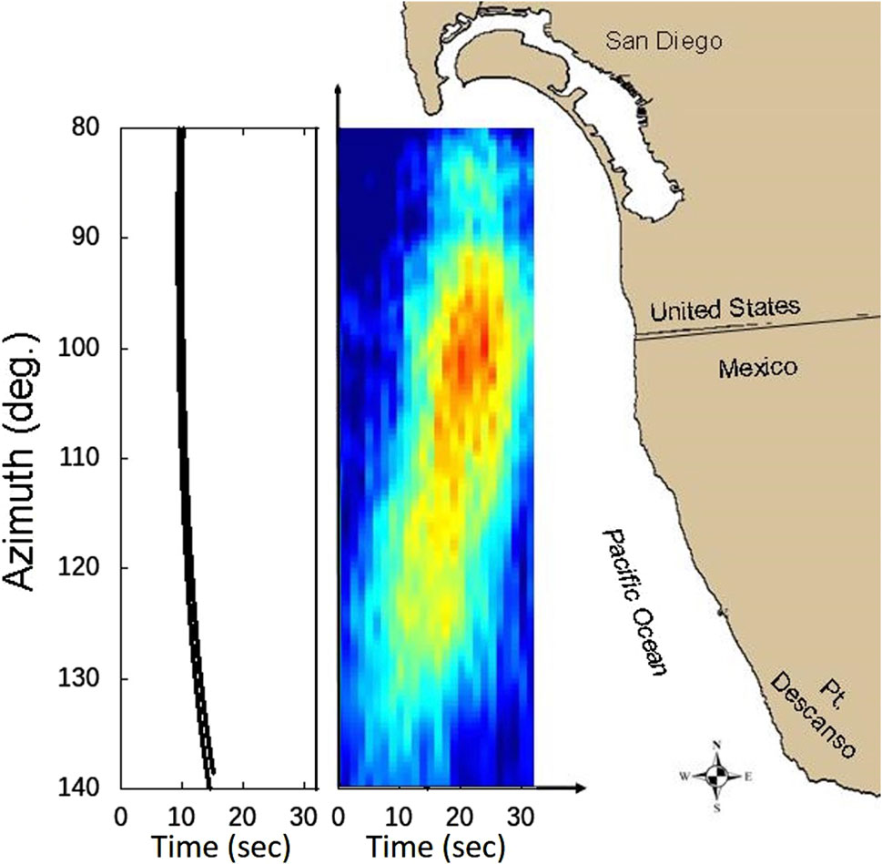
Figure 3. White-noise-constrained adaptive beamformer output showing one of the chorus cycles during SWellEx-1, superimposed on a map of the offshore San Diego/northern Mexico area. The beamformer output at each frequency was obtained using data from 28 elements of the 2D horizontal planar array and then incoherently averaged over the 400–450 Hz band, encompassing the peak in received spectral density level of the biological choruses. The plot covers a 32-s period spanning the look directions from 80° true (10° north of due east) to 140° true (southeast). The inset on the left of the figure shows the underwater acoustic travel time from the boundaries of the numerical simulation grid to the observation location (approximating the relative position of the SWellEx-1 array) as a function of azimuth of arrival on the same scale as the plot of the chorus cycle.

Figure 4

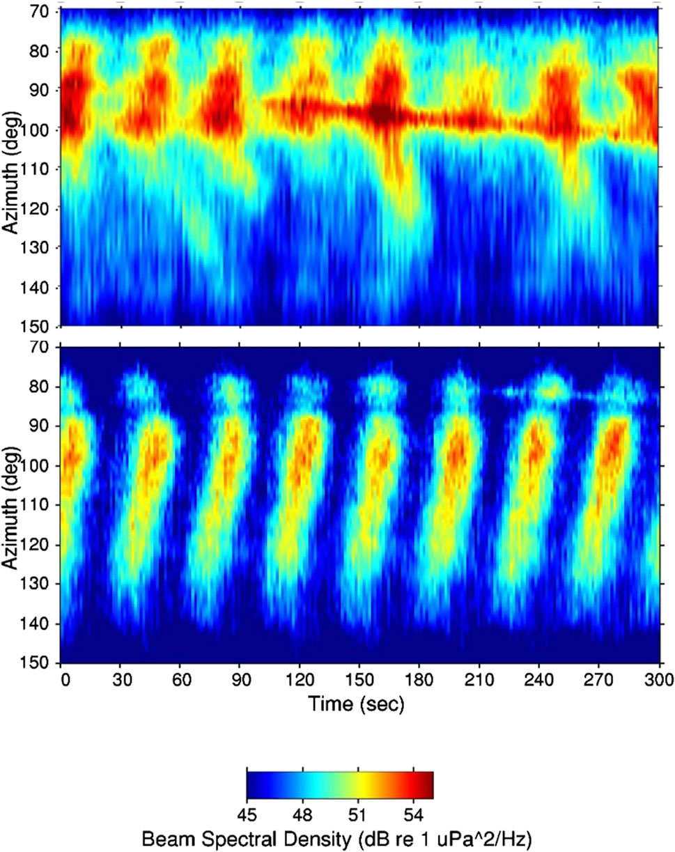
Figure 4. Adaptive beamformer output from the 2D horizontal planar array in SWellEx-1 for two different 5-min time periods. The sixth chorus cycle from the left in the lower plot, just after the 180-s mark, is the same one plotted in Figure 3. These 5-min data used the same 28 elements and were processed identically, including averaging over the 400–450 Hz band. These plots have a look-direction scale from 70° true to 150° true with a color scale running from 45 to 55 dB re 1 μPa²/Hz. Whereas the data in the lower plot were recorded in the darkness of the early morning hours (05:05:00–05:10:00 PDT), those in the 5-min period in the upper plot were recorded in the 05:45:45–05:50:45 PDT time interval, about a half-hour before local sunrise (which was at 06:14 PDT).

The region of coastline where the highest received levels arrive from (the red-colored patches) in Figure 3 and the lower plot of Figure 4 is approximately offshore of the Tijuana River outflow in southern San Diego County and the San Antonio de los Buenos Creek outflow in the northwest corner of Tijuana, Mexico. These outflows may increase the nutrients available for primary productivity offshore and so lead to an increase in some marine animal populations. At the other extreme are the low received levels in the direction of about 87° T, with the region northward of this direction (corresponding to the Silver Strand Peninsula coastline in San Diego) at times not strictly following the pattern to the south. This direction corresponds approximately to the direction of the Imperial Beach kelp forest (Figure 2 of Parnell et al., 2018; Figure 1 of Leichter et al., 2023). Sounds from this bioacoustics chorus also do not arrive from the direction of the kelp forests off Pt. Loma, creating the northern terminus of the chorusing region in Figure 3 and Figure 4 (see Fig. I.3 of D’Spain et al., 1997), nor do they come from the kelp forests just north of the ABM study site.

Around daybreak, the time period of the chorus cycles begins to increase as the maximum amplitude within a cycle decreases (see Fig. I.3 of D’Spain et al., 1997; Figure 4 of D’Spain et al., 2013). During this period, ships begin departing from San Diego Harbor. The upper plot in Figure 4 shows the beamforming results for a 5-min period about a half-hour before local sunrise, as a ship departs the harbor and heads south, forming the line running from 90° T at the left to 100° T at the right. Associated with this track are branches of received sound that evolve with time (to the right in the plot) with increasing azimuthal separation from the track. One possible explanation for this pattern is that the sound from the ship periodically stimulates chorusing with the region of chorusing progressively traveling up and down the coast, away from the ship, with time. That is, the animals that participate in this chorusing behavior appear to be sensitive to changes in received sound level and react by calling. This characteristic is the basis of the nonlinear coupling between units in the numerical modeling, as discussed in the previous section.

3.2 Signal processing

The data recording during SWellEx-1 was intermittent and the data quality in the first part of the experiment was low. In contrast, array data were recorded nearly continuously throughout the 2 weeks of the SWellEx-3 experiment and were of consistently high quality. Both experiments occurred at the same location with an offset in time-of-year of less than 1 month between the sea tests. Continuous spectrograms of a few array elements were created over the complete duration of SWellEx-3 to provide a pictorial representation of acoustic transmissions and background noise during the recording period to help guide the data analyses. A qualitative assessment of the spectrograms in the frequency band of the biological chorus is presented in Figure 5. The chorus occurs predominantly at night with significant changes in character around sunset and sunrise. The transition between continuous and cycling around sunset is particularly notable, and is a feature replicated by the numerical models as demonstrated in the next section.

Figure 5

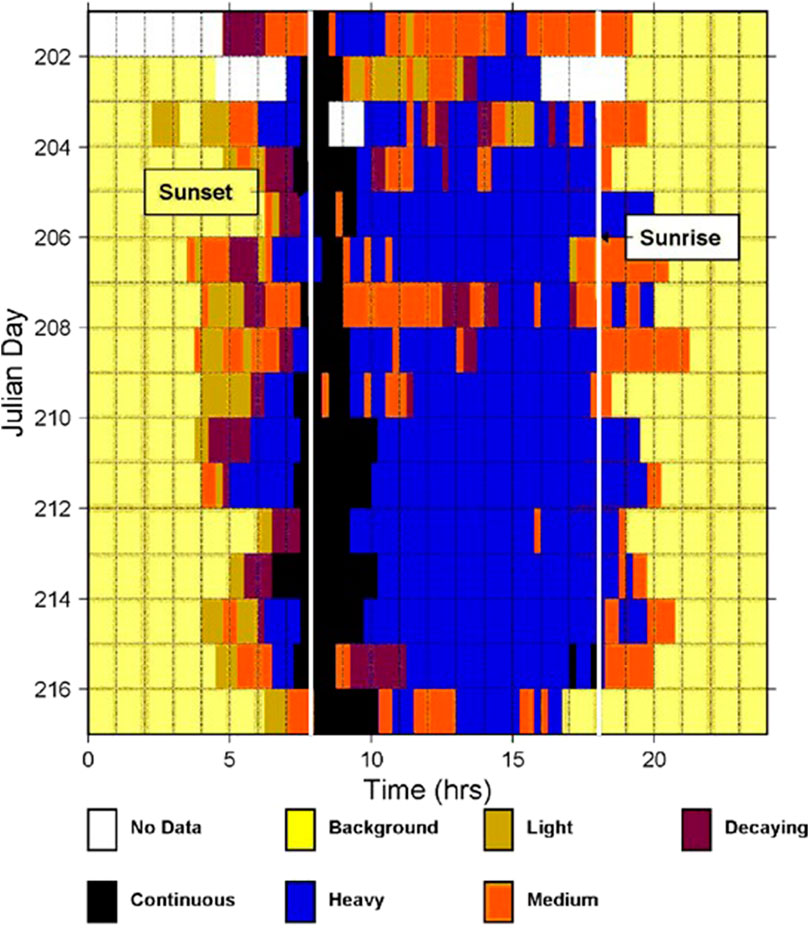
Figure 5. Qualitative assessment of the occurrence and character of the low frequency cycling chorus in the SWellEx-3 experiment, from JD 201 to 216 (20 July to 4 August), determined from one data analyst’s visual examination of the spectrograms from a single array element covering the 16 days of the experiment. SWellEx-3 was conducted the following year at the same location and season (summer) as SWellEx-1. The horizontal time axis starts at noon local time and spans 24 h. The terms “Heavy”, “Medium”, and “Light” are qualitative descriptors for the received levels of the cycling chorus, “Decaying” indicates an increase in the time between choruses as well as a decrease in received levels that occur around sunrise, and “Continuous” represents those periods primarily around sunset where the chorus sounds do not display the cycling variation in received levels. The vertical white lines indicate the times of local sunset and sunrise.

The individual sounds that comprise the biological chorus were recorded in the ABM-95 experiment where the bottom-mounted array location apparently corresponded with a region of chorusing (D’Spain et al., 1997). These sounds are composed of a sequence of 5–13 knocks that occur with a nearly constant inter-knock interval that can vary from 0.5 to 0.75 s from one sequence to the next. Fig. II.1 of D’Spain et al., 1997 shows a time series plot of one such “knocking” sequence of 10 knocks with an inter-knock interval of 0.7 s (repeated in the lower plot of Figure 6). The simplicity of these individual sounds allows them to be readily simulated as demonstrated by the synthetic waveform in the upper plot of Figure 6. Because each knock in a sequence has approximately the same amplitude (after correcting for changes in range of the animal from the recording hydrophone during the knocking sequence) and is followed by about the same interval of time before the next knock occurs, the mean squared amplitude of the sequence, $〈A^2〉,$ is independent of the number of knocks in the sequence and so equals the mean squared amplitude of a segment containing a single knock and inter-knock interval:

$〈A^2〉=\frac{{\displaystyle {\sum }_{i=1}^N}{a}_i^2}{∆t\bullet f_s+N}(11)$

Figure 6

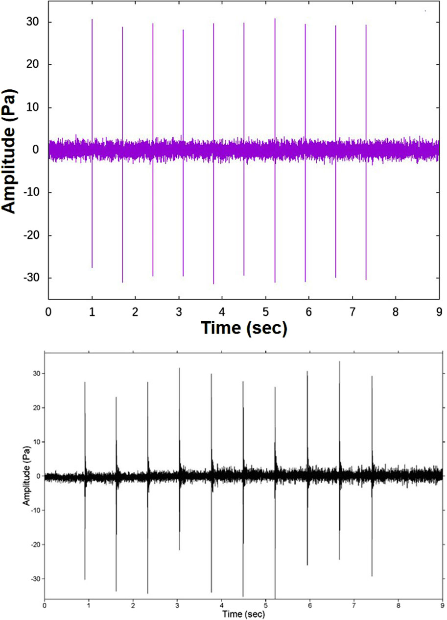
Figure 6. A synthetic time series over 9-s (upper plot), created to match the character of the measured 9-s time series plotted in Fig. II.1 of D’Spain et al., 1997 and copied here for reference (lower plot).

In this expression, $N$ is the number of data samples comprising the knock and $a_i$ is the amplitude of the $i^{th}$ data sample in the knock. The inter-knock interval of duration $∆t$ has $∆t\bullet f_s$ data samples at data sampling frequency $f_s.$ (Likewise, $N=t_s\bullet f_s$ where $t_s$ is the knock duration). A mean spectral density, $\overline{S_p}$ , averaged over the frequency band of the call can be derived as $\overline{S_p}=\raisebox{1ex}{$2〈A^2〉$}\!\left/ \!\raisebox{-1ex}{$f_s$}\right..$ This expression allows the rms source level to be readily derived from the peak source level for the knocking sequence. For knock amplitudes of ±30 Pa and a source-receiver distance of 2 m (D’Spain et al., 1997), the 0-peak source level is 156 dB re 1 μPa @ 1 m and the equivalent rms source level density is 100 dB re 1 μPa²/Hz @ 1 m. Therefore, the rms source level integrated over the 400–450 Hz band (used as input to the numerical modeling) is 117 dB re 1 μPa @ 1 m. The expression also allows the difference in rms source level between different sequences of knocks having different properties to be readily calculated. For example, for two sequences having identical properties except for inter-knock intervals of $∆t_1$ and $∆t_2$, the source level difference in the case where the inter-knock interval is much larger than the duration of a knock, as in these individual knocking sequences, the difference is $10\bullet \log \left(\raisebox{1ex}{$∆t_1$}\!\left/ \!\raisebox{-1ex}{$∆t_2$}\right.\right).$ This difference equals 1.8 dB for the two groups of knocking sequences having about 0.75 s and 0.5 s inter-knock intervals that were recorded in ABM-95.

Using single-element spectrograms covering the full duration of the ABM-95 experiment as a guide, the corresponding acoustic pressure time series for 6 nights spanning 19 days were searched for occurrences when a calling animal came sufficiently close to the recording element that its knocking sequence could be clearly distinguished from the background din (D’Spain et al., 1997). Results from this analysis are plotted in Figure 7. As discussed previously, the histograms of inter-knock intervals (left panel) divide into two distinct groups. The inter-knock intervals for both groups change in unison over the 6 nights, by an amount representing a maximum change in rms source level of 1.3 dB for both groups. Decreases in the inter-knock intervals are associated with increases in the overall chorus level measured at the time of the knocking sequence recordings (middle panel). However, changes in the inter-knock intervals alone are not sufficient to explain the maximum 7 dB change in chorus levels. The mean number of knocks in an animal’s sequence (right panel) also increase with increase in chorus level and decrease in inter-knock interval, although the association is weaker. The inverse relationship between inter-knock interval and number of knocks in a sequence tends to create a constant duration of calling.

Figure 7

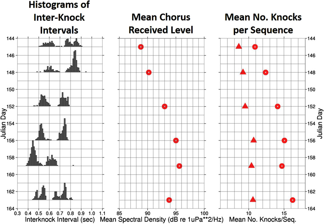
Figure 7. Histograms of the time intervals between successive knocks in a knocking sequence (left panel), the mean spectral density levels of the choruses in the 300–700 Hz band (center panel), and the mean number of knocks in a sequence (right panel) for 6 nights evenly spaced over 19 days in the ABM-95 experiment. The group of calls plotted with circles in the right-hand plot, showing a greater mean number of knocks in a call, corresponds to the group whose histograms in the left-hand plot have the smaller interknock intervals centered around 0.5 s. Likewise, the group with a smaller mean number of knocks in a call (plotted with triangles in the right-hand plot) corresponds to the group whose interknock interval histograms are concentrated above 0.6 s. In effect, the duration of calling for both groups tends toward the same value.

The properties of these individual animal sounds are used as input to the numerical modeling.

3.3 Numerical modeling

The input parameters to the numerical model are constrained to the extent possible by the observations from the SWellEx and ABM experiments, assuming the animals participating in the biological choruses are the same species. As mentioned above, the geometry used in the numerical modeling approximates that of the SWellEx-1 experiment, with the length along coast for the two-dimensional grid set at 20 km. In addition, the array location is 17 km from the southern end of the grid and 15 km offshore. Since the distance offshore and cross-shore width of the chorusing region are unknown, they were varied in the modeling. The water column sound is set to 1,500 m/s and the water depth to 20 m, corresponding to the water depth at the region of chorusing in ABM-95. The properties of the individual calls also are taken from the ABM-95 measurements; the rms source level over the 400–450 Hz band is equal to 117 dB re 1 μPa @ 1 m (see the previous subsection), the duration of calling, ${\tau }_{call}$, is equal to 5 s (re Figure 7 and corresponding discussion above), and the time period in the resting state, ${\tau }_{rest}$, is set to 30 s so that the periods of the chorus cycles obtained from the numerical modeling output approximately equal those observed in the data (discussed further below). The spatial density of animals, ${\rho }_s$, is adjusted so that the received sound levels output by the model approximately match those measured in the experiments (see Discussion below). The remaining input parameters are the four parameters in Eq. 8, ${\gamma }_{\mathit{max}}$, ${\gamma }_{\mathit{min}}$, $R{L}_{tran}$, and ${\sigma }_{RL}.$

The rate of units transitioning from excitable to the calling state, $\gamma ,$ (or equivalently, $\raisebox{1ex}{$1$}\!\left/ \!\raisebox{-1ex}{$\gamma $}\right.$ , the mean time spent in the excitable state) is the variable that controls the stochastic behavior of the system. The expression for this variable used in the modeling is given in Eq. 8. To illustrate the effect of variations in the four input parameters in Eq. 8 and their inter-relationships, a series of plots was created. Two such plots are presented in Figure 8. The left-hand plot of the mean time spent in the excitable state as a function of received sound level and coupling parameter ${\sigma }_{RL}$ indicates that 1) as the received level increases at a fixed ${\sigma }_{RL}$, the mean time in the excitable state decreases and the system becomes more deterministic, and 2) the same result holds as the coupling parameter increases at fixed received level. An abrupt transition to negligible mean times occurs at the transition received level, $R{L}_{tran}$, particularly evident at the smaller values of ${\sigma }_{RL}$ . Changes in the value of ${RL}_{tran}$ simply shifts the pattern of the plot in Figure 8 horizontally. Other combinations of input parameters yield plots that are nearly identical to the left-hand plot in Figure 8. For example, a plot of $\raisebox{1ex}{$1$}\!\left/ \!\raisebox{-1ex}{$\gamma $}\right.$ as function of received level over the same 50–150 dB range and ${\gamma }_{\mathit{max}}$ from 0.1 to 10 1/sec at fixed values of ${\gamma }_{\mathit{min}}=0.1$ 1/sec, ${\sigma }_{RL}=3.0$ dB, and ${RL}_{tran}=130$ dB looks just like the left-hand plot in Figure 8. Therefore, the four input parameters are inter-dependent and appropriate combinations of parameters yield the same result (as expected since four input parameters determine a single output value).

Figure 8

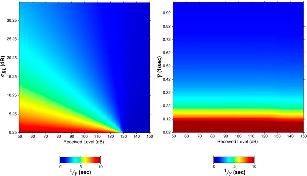
Figure 8. Plots of the mean time in the excitable state (the inverse of Eq. 8) as a function of received sound level (horizontal axis) and (A) ${\sigma }_{RL}$ (vertical axis) at fixed ${\gamma }_{\mathit{max}}=2.0$ 1/sec and ${\gamma }_{\mathit{min}}=0.1$ 1/sec, and (B) $\overline{\gamma }\equiv \left({\gamma }_{\mathit{max}}+{\gamma }_{\mathit{min}}\right)/2$ (vertical axis) at fixed $∆\gamma \equiv {\gamma }_{\mathit{max}}-{\gamma }_{\mathit{min}}=0.01$ 1/sec and ${\sigma }_{RL}=3.0$ dB. In both plots, the value of $R{L}_{tran}$ is set to 130 dB.

The right-hand plot in Figure 8 shows the effect on $\raisebox{1ex}{$1$}\!\left/ \!\raisebox{-1ex}{$\gamma $}\right.$ of varying received level and $\overline{\gamma }$ while keeping $∆\gamma$ and ${\sigma }_{RL}$ fixed in value. Under these conditions, the mean time in the excitable state decreases with increasing $\overline{\gamma }$, as expected, but does so approximately independent of received level. Specifically, changes in received level around ${RL}_{tran}$ and changes in the value of ${RL}_{tran}$ itself have no discernible effect. Therefore, the sensitivity of the excitable system response to changes in a given input parameter is dependent on the conditions and values of the other input parameters to Eq. 8.

Before proceeding to running simulations with the full model, the effect of the acoustic received level on the rate of transition from excitable to active was disabled in the code so that fixed values for $\gamma$ could be used in place of Eq. 8. The results from one set of runs are presented in Figure 9. The second 5-min period is displayed to exclude the transient effects that occur at the start of a simulation. The fraction of calling units in the left-hand plot indicates that at the larger values of $\gamma ,$ all units call nearly simultaneously and are silent (either resting or in the excitable state) in unison. The time between the cycles matches the period of the chorus cycles in Figure 4 as a result of the appropriate choice for ${\tau }_{rest}$, as mentioned above. As the value of $\gamma$ decreases, the cycle period increases until around $\gamma =0.05$ where the cycling nature of the chorus begins to disappear. This phenomenon reproduces the transition between the continuous sunset chorus and the night-time cycling chorus (Figure 5). The simulated received sound levels over the same 5-min period (right-hand plot of Figure 9) show a similar effect, although the peaks in received level are broader than those for the fraction of calling units and the pattern is shifted in time slightly. Both differences are caused by the travel-time delays in sound propagation from locations in the 2D grid to the array location (as in the inset on the left of Figure 3). The transition from cycling sound levels to a continuous din around $\gamma =0.05$ 1/sec corresponds to a mean time in the excitable state, $\raisebox{1ex}{$1$}\!\left/ \!\raisebox{-1ex}{$\gamma $}\right.$, of around 20 s and a standard deviation in this mean time of the same amount, so that both quantities are approaching the total time to complete one cycle.

Figure 9

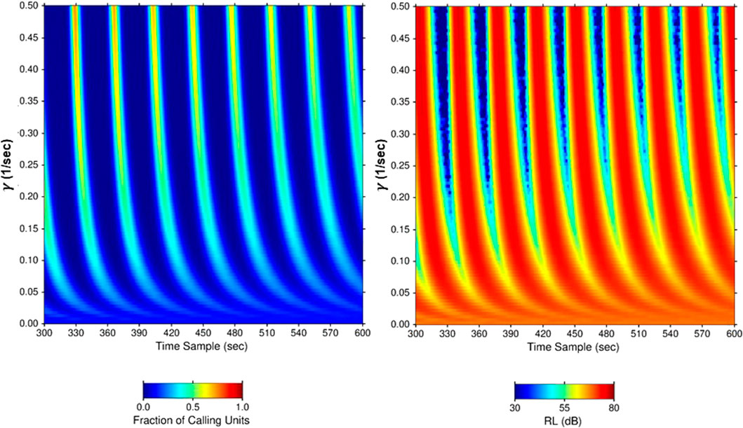
Figure 9. Simulation results for fixed input values of $\gamma$, the rate of transitioning from the excitable to calling states. The left-hand plot shows the fraction of calling units and the right-hand plot is the corresponding received sound level at the approximate array location in SWellEx-1. The axes are the same in both plots—the horizontal axis is time over the 5–10 min period after initiation of the simulation (each time sample is 1 s) and the vertical axis spans 100 input $\gamma$ values from 0.005 1/sec to 0.5 1/sec.

The remaining results presented in this subsection were obtained from the full model. An important aspect in running the simulations is the state of the units at the start. A variety of initial conditions were used. If all units start in the same condition, i.e., at the same stage in the same state, the resulting received levels versus time do not correspond to the measurements. Alternatively, if the time each unit was last active is chosen from a uniform probability distribution with bounds $\left.\left[-{\tau }_{rest},0\right]\right]$, i.e., between just entering the excitable state and just entering the resting state, then the cycling nature of the chorus levels can be replicated with the appropriate choice of input parameters. However, the evolution upcoast of the region of chorusing over time as seen in Figure 3 and Figure 4 did not occur, even after numerous runs and after activating an external sound source at the left-hand (southern) end of the spatial grid at the start of the simulation. The unusual spatiotemporal evolution of the chorus was achieved by applying a weighting to the randomly chosen time that each unit was last active, with the weights starting at unity and decreasing linearly with distance upcoast. The result of this weighting in initial state for one simulation is shown in Figure 10. The stack of 10 two-dimensional spatial grids illustrates the increase in calling units (purple dots) and the evolution of their locations upcoast over a 25-s period starting at the beginning of the simulation.

Figure 10

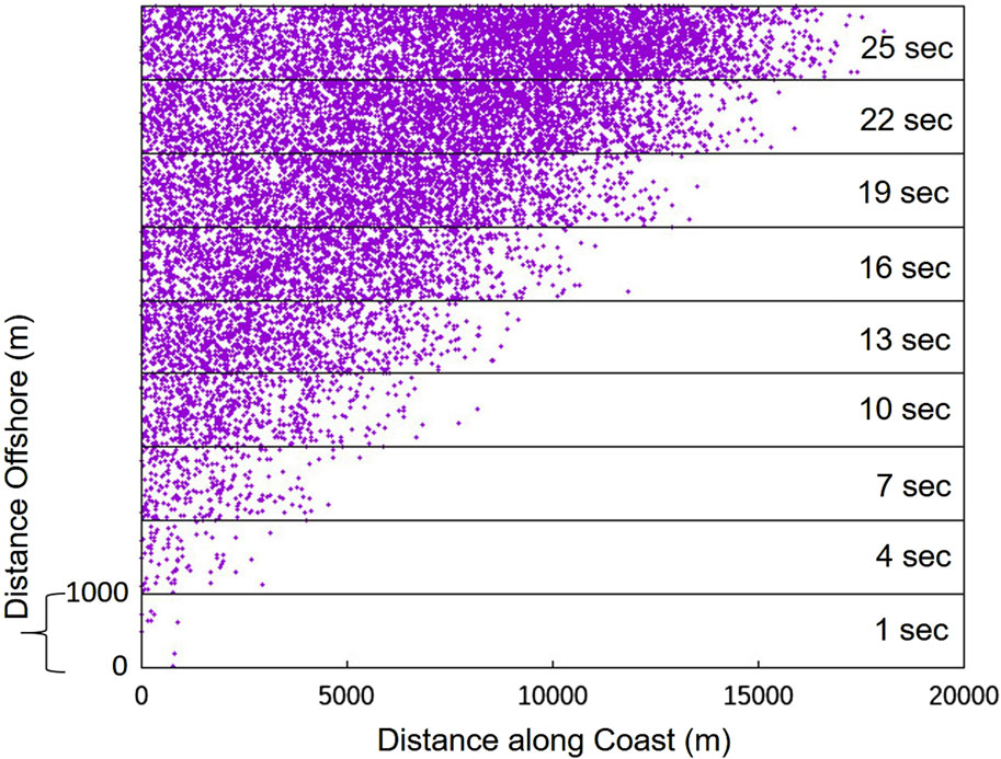
Figure 10. A stack of 10 two-dimensional spatial grids, with each grid representing 20,000 m in the horizontal and 1,000 m vertically. Each 2D grid is a snapshot in time showing the locations of active (calling) units (purple dots). The time snapshots are sequential in time and spaced every 3 s as indicated on the right side of the plot.

For the same simulation as in Figure 10, the modeled evolution of the directionality of the chorus sounds over a 5-min period at the approximate SWellEx-1 array site is presented in the right-hand plot of Figure 11. The chorus peaks in this plot successfully replicate the tilted appearance of the measured chorus peaks in Figure 3 and Figure 4. The simulated peaks are not as broad as the measured cycle peaks because the spatial filtering characteristics of the 2D horizontal array (right-hand plot in Figure 2) have not been applied to the simulation results.

Figure 11

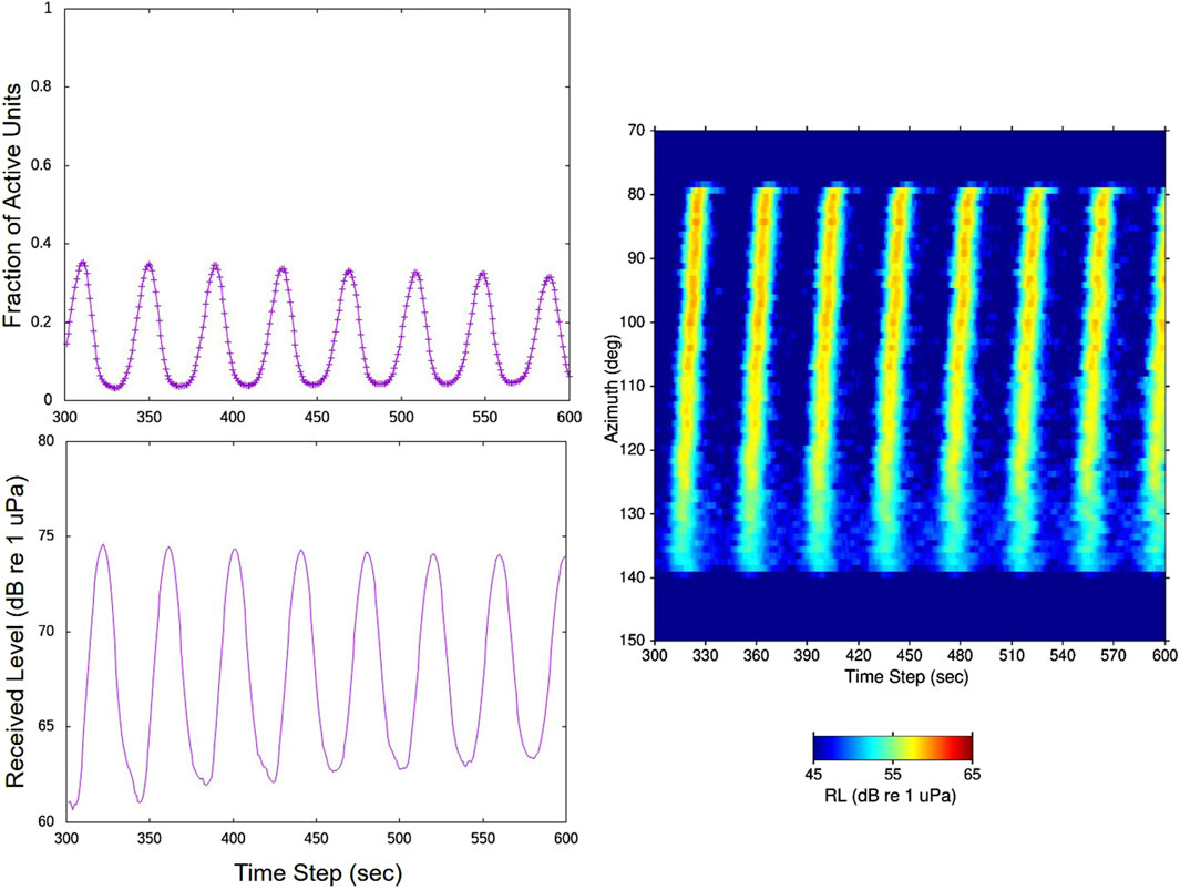
Figure 11. Results from the same simulation as in Figure 10. The upper-left plot is the fraction of calling units over the second 5-min time period of the simulation and the lower-left plot is the corresponding received sound level over the same 5-min period for an omni-directional receiver at the approximate array location in SWellEx-1. The directionality of the received sound over this 5-min period is displayed in the right-hand plot. The received levels are integrated over the 400–450 Hz band, so that 17 dB (=$\left.10\bullet {\log }_{10}\left(450-400\right)\right)$ should be subtracted from these values to obtain the received spectral density.

The plots on the left-hand side of Figure 11 of the fraction of active units and received sound level at the approximate array location over the same 5-min period display the cycling character seen in the data. Again, the peaks and troughs in the received level plots lag in time by order 10 s from those in the plot of the fraction of calling units as a result of the acoustic propagation delays across the 2D grid to the array site.

Results from a different full model simulation are displayed in Figure 12. The input parameters here were identical to those for the simulation in Figure 10 and Figure 11 except for an increase in the value of $R{L}_{tran}$, the transition received level; from $R{L}_{tran}=108$ dB to $R{L}_{tran}=130$ dB. Although both the fraction of calling units and received level plots show a weak oscillatory behavior, it is decaying and asymptotically approaching steady-state values, replicating the chorus character during the sunset chorus. The modeled omnidirectional received sound levels for a location in the center of the 2D spatial grid reach peaks in the range 105–110 dB re 1 μPa for this simulation, resulting in maximum rate-of-transition values of $\gamma \cong 0.025$ per sec. Figure 9 shows that rate values this small result in continuous rather than oscillatory behavior. In contrast, for the results in Figure 11, the maximum rate values are around 0.129 per sec where Figure 9 indicates oscillatory behavior occurs. Simulation results that best match the experimental measurements are achieved at transition received levels of $1{\sigma }_{RL}$ above peak received levels within the 2D spatial grid (chorusing region) for the other selected input parameters to Eq. 8.

Figure 12

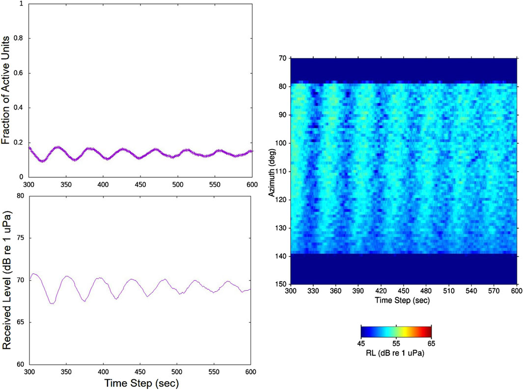
Figure 12. Results from a different simulation than Figure 11 in which the only change was to increase the input value of $R{L}_{tran}$ from 108 dB to 130 dB. This figure has the same format and all plots have the same scale as those in Figure 11 to aid comparison.

Finally, Figure 13 presents the direction-of-arrival versus time plots for two additional simulations. Both simulations used exactly the same input parameters as those in Figure 11 except that the spatial density of animals, ${\rho }_s$, was reduced from 1,000 to 100 animals per km². In addition, the track of a ship (clearly seen in the left-hand plot as it transited from 90° T to 100° T over the 5-min period) was included in the analysis on the left in order to simulate the transiting ship in the upper plot in Figure 4. The radiated noise from the transiting ship has a significant impact on the spatiotemporal characteristics of the biological chorus, as comparison of these plots and those in Figure 4 show. Rather than steadily evolve from south to north when an external noise source is not present, the region of chorusing tends to evolve upcoast and downcoast away from the ship track. In addition, for the left-hand plot in Figure 13, the ship noise leads to a concentration in the time of calling of the animals in the vicinity of the ship into a shorter time period in each chorus cycle, so that the peak levels in each cycle around the ship are higher and tend to appear like those in Figure 11. The reason for this concentration is that the higher received levels from the ship noise cause the individual units to spend less time in the excitable state. Increases in sound level from other calling units when the spatial density of units is greater have the same effect, as shown in the simulation in Figure 11. (When a transiting ship is introduced into a simulation under the same conditions as those for Figure 11, specifically a spatial density of 1,000 units per km², the region of chorusing changes to evolve in the same way as in the left-hand plot of Figure 13. However, the concentration in time of calling remains the same as in Figure 11). In contrast, the peak levels in each chorus cycle in the right-hand plot are more diffuse in time, similar to those in Figure 12, indicating a greater variability in time spent being excitable. This similarity suggests that decreases in the spatial density of excitable units has a similar effect as increases in the value of the transition received level $R{L}_{tran}$; both lead to decreases in the value of $\gamma \left(RL\right)$.

Figure 13

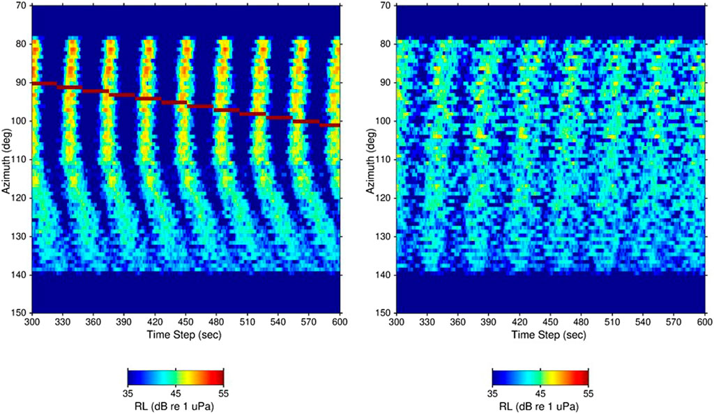
Figure 13. Direction-of-arrival over a 5-min time period for two simulations having the same inputs as the simulation in Figure 11 except that the spatial density of units is reduced from 1,000/km² to 100/km². As a result, the color-scale of the two plots is reduced from that in Figure 11 by 10 dB (=$\left.10\bullet {\log }_{10}\left(1000/100\right)\right)$. In addition, a ship with source level of 180 dB re 1 μPa @ 1 m transited from north to south (along-coast) at 10 m/s (19.4 kt) over the 600-s duration of the simulation generating the left-hand plot.

4 Discussion

An underwater bioacoustic chorus with unusual spatiotemporal properties has been recorded in the nearshore regions off the southern California coast. The direction of the active chorusing region during one experiment evolved upcoast indicating a speed of migration of the chorusing region one hundred times faster than the 12 m/s of human waves in sports stadiums (Farkas et al., 2002), approximating the 1.5 km/s speed of sound in water. With the appropriate inputs, a numerical model based on the physics of excitable media can reproduce many of the measured features of the chorus.

Many of the input parameters to the numerical models are determined, or at least constrained, by the environmental setting and ocean acoustic measurements collected during the SWellEx and ABM-95 experiments. This approach assumes that the bioacoustics results from the ABM-95 experiment, whose location is 75 km upcoast from the SWellEx site, also reflect the soniferous properties of the animals in the nearshore region south of the mouth of San Diego harbor. The basis for this assumption is that the choruses at both sites have the same frequency content, the same dependence on time of day, and the same oscillatory nature in received sound levels. The two populations of animals that create the choruses, although possibly from the same family, may not be of the same species, as discussed further below.

Three components of the numerical models are stochastic; 1) the number and location of the units in the 2D spatial grid based on an input unit spatial density (i.e., number of units per square area), 2) the state and the time of entry into that state of each unit at the start of a simulation, and 3) the transition probability from the excitable to active/calling state. This transition probability is based partly on the time a given unit already has spent in the excitable state and partly on the received sound level. Regarding the latter aspect, it has long been recognized that males of certain species of fish generate sound during spawning season (e.g., Winn, 1964). They may be in acoustic reproductive competition with other males, responding to received sound levels above a threshold by calling in turn. Evidence of this acoustic response to received sound is suggested by the results Figure 7, in which characteristics of the individual calls change in association with changes in overall chorus level. Some indication also is available from the spatiotemporal evolution of the chorus region associated with the tracks of ships departing from San Diego harbor after sunrise; it appears that the noise from the ship stimulates the animals nearby into chorusing which then stimulates chorusing by individuals at progressively farther distances up and down the coast (the upper panel of Figure 4 presents one example).

To successfully model this underwater acoustic version of “The Wave”, the starting conditions for each simulation must be set appropriately. In this work, the initial, randomly-selected time that each unit was last active (no unit starts in the active state) is linearly weighted by that unit’s distance upcoast. Tom Norris of BioWaves suggested a naturally occurring source that could give rise to conditions that mimic this initial state—the sound of breaking surf from long-period swell from the south-westerly direction (private communication, 2006). The periodicity of the chorus evolution upcoast is on the same order as that of long-period ocean swell. One of the anonymous reviewers of this paper offered a second hypothesis—that changes in the time of sunset with increasing latitude at this location at this time of year may create the appropriate starting conditions for “The Wave”. Figure 5 clearly illustrates that the chorus starts around sunset and occurs almost exclusively during the hours of darkness. Using the online sunrise/sunset calculator at https://planetcalc.com/874/, which implements the algorithm published by Montenbruck and Pfleger (1994, 2013), an increase of 1° of latitude results in a nearly 1-min increase in the time of sunset. Therefore, over the 20 km south-to-north extent of the modeled chorusing region, sunset time increases by more than 10 s. This increase is strikingly similar to the time it takes the chorus to travel the same upcoast distance and with ocean swell periods. In addition, the correspondence of a) the time it takes for the region of peak chorusing levels to travel upcoast and then start again at the downcoast end with b) the period between one chorus peak and the next in the cycle as measured at a single location (as in the single element spectrograms in Fig. I.1 of D’Spain et al., 1997 and Figure 2 of D’Spain et al., 2013) likely is not coincidental. In fact, this correspondence may be one of the important factors that determines the spatial extent of coastline that can participate in “The Wave” phenomenon. Note that this unusual spatiotemporal evolution was not observed in the measurements reported in D’Spain et al., 2013.

Once the upcoast evolution of the chorusing region is initiated at the start of a simulation, it must repeat cycle after cycle to reproduce the character of the lower plot in Figure 4. After a given cycle is completed at the upcoast terminus, the region at the southmost part of the grid is not exposed to the sounds from nearby calling animals to trigger calling (i.e., increase the probability of transitioning from the excitable to active states). Therefore, the value of ${\gamma }_{\mathit{min}}$ in Eq. 8 must be sufficiently large so that the time since last calling will trigger the transition. This situation differs from the “closed circuit” conditions of spiral waves in excitable media (Greenberg and Hastings, 1978), and the continuous ring of spectators in a stadium that participate in “The Wave” (Farkas et al., 2002).

By comparing the simulated received levels at the approximate SWellEx-1 array site to those measured in the experiment, and/or the simulated levels in the middle of the spatial grid to those measured in the ABM-95 experiment (re Fig. I.2 of D’Spain et al., 1997), appropriate input values for the spatial density of animals, ${\rho }_s$, can be determined. Simulations show that the received levels at both measurement sites increase approximately 3 dB with a doubling of the spatial density, as expected for incoherent summation of individual sounds, allowing ${\rho }_s$ to be readily adjusted. The comparison with ABM-95 data suggests a density of around 2000 animals per square km, and a number somewhat larger for SWellEx-1. One weakness with the latter comparison is that the transmission loss between the chorusing regions and the SWellEx-1 array location was never measured to validate the transmission loss model in Eq. 10. For the ABM-95 comparison where the reference receiver is located within the region of chorusing, the modeled received levels vary widely from one simulation to the next because of the variability in the number of units in closest proximity to the selected receiver location. Averaging a large number of simulation results for reference receivers at different locations in the grid along with a corresponding averaging of received levels over time measured by ABM array elements across the full array length would reduce this variability. In any case, the measurements in the SWellEx and ABM-95 experiments cannot be used to reliably estimate the spatial density of the animals participating in the chorus—the experiments were not designed for this purpose.

Inter-comparison of the two plots in Figure 13 (as well as those in Figure 4) suggest that the radiated noise from a transiting ship can impact the acoustic behavior of the animals participating in the biological chorus. Studies on a species of fish in the croaker (Sciaenidae) family (the same family that the animals participating in the chorus here are hypothesized to be from, as discussed in the next paragraph) found that characteristics of their calls (mean pulse rate) changed to compensate for repeated exposures to noise from recreational boat transits (Picciulin et al., 2012). These results also are compatible with the associations between changes in mean chorus level and changes in both inter-knock interval and mean number of knocks in a call illustrated in Figure 7; the animals’ vocalizations appear to adapt to changes in the ocean soundscape. However, the possibility that manmade noise can adversely impact these animals is highly speculative at this point, although worth investigating further. To quote the final sentence in the Conclusions of the Picciulin et al. paper “At the same time, it also indicates that there are many open questions that need to be answered to fully understand the relationship between fish vocal behavior and anthropogenic noise.”

The species of animals that participate in this underwater chorusing behavior off the southern California coast is unknown. However, evidence gathered from the ocean acoustic experiments and other sources of information can help narrow the candidates. The hydrophone array recordings indicate the directions of the chorusing regions are towards the nearshore, shallow waters overlying sandy bottom areas. No chorusing sounds appear to come from the directions of the kelp forests just west of Pt. Loma (the gap in chorusing sounds coming from the azimuthal interval of about 10° to 80° T in Fig. I.3 of D’Spain et al., 1997), off Imperial Beach (the gap around 87° T in Figure 3 and the lower panel of Figure 4), or just north of the ABM site (unpublished results from ABM-95). The chorus sounds apparently occur only in the spring and summer months (the spawning season for many species of fish) since during an experiment conducted at the ABM site in the November time period, no significant biological sounds of this nature were recorded. The chorus only occurs at night, as illustrated in Figure 5. These characteristics correspond to the behaviors and spatial distributions of certain fish species found off the southern California coast (Goodson, 1988). The sound-producing characteristics of a wide variety of fish species have been studied for over a half-century (e.g., Tavolga, 1964), and members of the croaker (Sciaenidae) family are now well-known producers of underwater sound. The spatial and temporal abundance of various sound-producing fishes off the southern California coast including croakers can be gleaned from several different sources. For example, the California Cooperative Oceanic Fisheries Investigations (CalCOFI) reports and atlases contain data on fish larvae and egg counts for various fish species, including those of the croaker family, collected during their quarterly surveys (Moser et al., 2001). The Allen et al. (2003) project report provides a list of sources of information on nearshore fish species and abundance off the southern California coast, specifically the bycatch data from SONGS and the four other power generating stations operated by the Southern California Edison Company, trawl survey data, and data from recreational fish catch surveys (pgs. 265–267). The entrapment data collected at SONGS provide a time series of the relative abundance of croaker species near the ABM site (Miller et al., 2011). The four most abundant croaker species in the bycatch are queenfish (Seriphus politus), yellowfin croaker (Umbrina roncador), white croaker (Genyonemus lineatus), and spotfin croaker (Roncador stearnsii). Queenfish and white croaker likely are the contributors to the choruses recorded at the ABM site because of their shared range that includes the northernmost part of San Diego County. These species also may be responsible for the choruses recorded at the SWellEx site. However, since yellowfin and spotfin croaker “are most commonly encountered in the more southern areas of the Southern California Bight, often in San Diego County and along the coastline of Baja California, Mexico” (Miller et al., 2011), it is possible they are the major contributors in this region. As discussed in D’Spain et al., 1997, given that only the males of a soniferous species typically create high, sustained levels of sound, then the dual nature of the histograms of the time interval between the knocks in an individual call (see the left panel in Figure 7) suggests that two anatomically similar species participate in the chorusing behavior. If so, the queenfish/white croaker pair may be responsible for the chorusing measured at the ABM site, whereas the yellowfin/spotfin pair may have created the underwater acoustic “Wave” recorded during SWellEx-1.

To conclude, it is important to put the numerical modeling results into context. The paper presents the development of a model to replicate many of the unusual patterns and features of the biological chorus that is based on reasonable underlying mechanisms. If the assumption is valid that the animals participating in the chorus react to characteristics of the received sound field (e.g., higher sound levels) by calling in turn, then this reaction provides a non-linear coupling mechanism between animals. Therefore, the collection of animals participating in the chorus comprises an excitable medium and the physics of excitable media provides an appropriate framework for studying their collective acoustic behavior. A cellular automaton approach often is used to numerically model phenomena in such complex systems (e.g., Gerhardt et al., 1990; Greenberg and Hastings, 1978; Murray and Murray, 1993; 2003; Lindner et al., 2004; Szakály et al., 2007). However, the mathematical formulation used in this paper to represent this coupling, as given in Eqs 4, 5, 8, is ad hoc. It is based on a modified version of a Poisson process, often used in statistics to model waiting times (e.g., Breiman, 1969), along with a modified version of Eq. (71) of Lindner et al. (2004). Eq. 8 was designed to have the following properties: a) upon first entering the excitable state, the probability of immediately transitioning to the calling state should be small when the received sound level is low, and reasonably large when the received levels are high, b) changes in received sound levels both at very low levels and at very high levels should not cause significant changes in the probability of transitioning, and c) the probability of transitioning at a given time after entering the excitable state should evolve smoothly with changes in received level between these two extremes in received level. Possibly the simplest formulation for $\gamma \left(RL\right)$ that combines all these factors is a piecewise linear function with three segments—a flat (insensitive) segment at very low received levels followed by a ramp from this low value to a higher value that connects to the third, flat (saturation) segment, at very high received levels. Eq. 8 approximates this piecewise linear function with a form that is not only continuous but continuously differentiable.

Other formulations of this coupling could be considered. In fact, one that was used in the initial stages of model development assumed that the two factors determining the transition from excitable to calling, i.e., the time since entering the excitable state and the received sound level, act separately and are statistically independent. Although the form for the coupling is ad hoc, the objective to replicate unusual features of the biological chorus was successfully met, indicating that only some non-linear coupling exists between units, and not the details of the coupling itself, was the key component to include in the model at this stage.

In advanced development of a numerical model for some physical phenomenon, the underlying physics of the phenomenon must be well understood. Analogously, to further model development in this case, the biological characteristics of the animals participating in the chorus should guide the derivation of the mathematical form for the non-linear coupling. This model advancement would greatly benefit from identifying the individual species, or set of species, creating the chorus. Experiments then could be conducted to address issues relevant to the coupling. For example, one question would be whether individual animals respond to changes in overall received sound level, as modeled here, or only to those components of a received sound field with properties (e.g., inter-pulse interval) that signify the sound was generated by a conspecific. (Changing the model to accommodate this latter possibility would be straightforward). The values for the input parameters to the mathematical expression for the coupling (for example, the four parameters in Eq. 8, ${\gamma }_{\mathit{max}}$, ${\gamma }_{\mathit{min}}$, $R{L}_{tran}$, and ${\sigma }_{RL}$) also could be determined or at least better constrained. Another interesting question is whether the mathematical form of the coupling applies to other species that mutually interact acoustically, requiring only adjustments to the parameters input to the coupling, or does the mathematical form itself need modification.

As with physics-based numerical models for physical phenomena that provide sufficient predictive capability with the appropriate inputs, a biologically-based numerical model of the chorusing could be used to invert a set of measurements for relevant properties of the chorusing animals. Even at the stage of model development presented in this paper, tentative results can be derived. One example, discussed above, is the inversion of chorus levels for the spatial density of calling animals. As another example, the periodicity of the chorus cycles suggests the animals enter a resting state after calling of around a half-minute duration before again becoming excitable. An interesting question to address in the future would be how this result might be biologically significant (does it aid in predator avoidance, relate to the energetics of an individual animal, somehow improve the chances of reproductive success during spawning, etc.).

By taking a first step in the development of a numerical model of biological chorusing, this work may have important applications to passive monitoring of certain nearshore environmental ecosystems, including the potential impact of human activities, and determination of essential fish habitats and spawning grounds.

Data availability statement

The computer code used to generate the simulations is available to any interested party upon request to the corresponding author.

Author contributions

GD: Conceptualization, Data curation, Formal Analysis, Funding acquisition, Investigation, Methodology, Project administration, Resources, Supervision, Visualization, Writing–original draft, Writing–review and editing. GR: Formal Analysis, Project administration, Writing–review and editing. HB: Formal Analysis, Investigation, Writing–review and editing. DR: Data curation, Formal Analysis, Investigation, Software, Visualization, Writing–review and editing.

Funding

The author(s) declare that financial support was received for the research, authorship, and/or publication of this article. All data collection and most of the analyses were conducted in a variety of research programs funded by the Office of Naval Research, Code 32. Publication costs were paid for by GLD.

Acknowledgments

This paper is dedicated to the memory of Lewis P. Berger, formerly at the Scripps Institution of Oceanography (SIO). Lewis worked with the authors of this paper on the original analyses of the experimental data. Thank you to Joe Rice, who along with his colleagues at the Space and Naval Warfare Center (SPAWAR), San Diego, was instrumental in SWellEx data collection. In addition, Mark Stevenson of SPAWAR participated in both SWellEx and ABM-95 experiments. Tony M. Richardson wrote the beamforming software while at SIO, and Jim Murray, formerly at SIO, improved the array and data processing software and was a central person in data collection in the three experiments. The array was designed, constructed, and deployed by engineers from the McDonnell Douglas Corporation, now part of Boeing. The original efforts at numerical modeling of the SWellEx biological chorus were presented at the June 2006 and June 2008 Acoustical Society of America meetings. Funding for all experiments and data analysis efforts was provided by the Office of Naval Research, Code 32. Their financial support is greatly appreciated.

Conflict of interest

The authors declare that the research was conducted in the absence of any commercial or financial relationships that could be construed as a potential conflict of interest.

Publisher’s note

All claims expressed in this article are solely those of the authors and do not necessarily represent those of their affiliated organizations, or those of the publisher, the editors and the reviewers. Any product that may be evaluated in this article, or claim that may be made by its manufacturer, is not guaranteed or endorsed by the publisher.

References

Allen, M., Smith, R., Jarvis, E., Raco-Rands, V., Bernstein, B., and Herbinson, K. (2003). Temporal trends in southern California coastal fish populations relative to 30-year trends in oceanic conditions. So. Calif. Coast. Water Res. Proj. Annu. Rept., 264–285.

Google Scholar

Breiman, L. (1969) Probability and Stochastic Processes: With a View Toward Applications. Boston, MA: Houghton Mifflin Company, p.324.

Google Scholar

Capon, J. (1969). High-resolution frequency-wavenumber spectrum analysis. Proc. IEEE 57 (8), 1408–1418. doi:10.1109/proc.1969.7278

CrossRef Full Text | Google Scholar

Cato, D. H. (1978). Marine biological choruses observed in tropical waters near Australia. J. Acoust. Soc. Am. 64 (3), 736–743. doi:10.1121/1.382038

CrossRef Full Text | Google Scholar

Clapp, G. A. (1966). “Periodic variations of the underwater ambient noise level of biological origin off Southern California,” in NEL Tech. Memo. 1027 (San Diego, CA: U. S. Navy Electronics Laboratory).

Google Scholar

Cox, H., Zeskind, R. M., and Owen, M. M. (1987). Robust adaptive beamforming. IEEE Trans. Acoust. Speech Signal Process. ASSP 35 (10), 1365–1376. doi:10.1109/tassp.1987.1165054

CrossRef Full Text | Google Scholar

D’Spain, G. L., and Batchelor, H. H. (2006). Observations of biological choruses in the Southern California Bight: a chorus at mid-frequencies. J. Acoust. Soc. Am. 120 (4), 1942–1955. doi:10.1121/1.2338802

PubMed Abstract | CrossRef Full Text | Google Scholar

D’Spain, G. L., Batchelor, H. H., Helble, T. A., and McCarty, P. (2013). New observations and modeling of an unusual spatiotemporal pattern of fish chorusing off the Southern California coast. Proc. Meet. Acoust. 19 (1), 010028. AIP Publishing, 7 pgs plus 5 figs. doi:10.1121/1.4800997

CrossRef Full Text | Google Scholar

D’Spain, G. L., Berger, L. P., Kuperman, W. A., and Hodgkiss, W. S. (1997). “Summer night sounds by fish in shallow water,” in Proc. Int. Conf. on Shallow Water Acoustics Editors R. Zhang, and J. Zhou (Beijing, China: China Ocean Press), 379–384.

Google Scholar

Farkas, I., Helbing, D., and Vicsek, T. (2002). Mexican waves in an excitable medium. Nature 419, 131–132. doi:10.1038/419131a

PubMed Abstract | CrossRef Full Text | Google Scholar

Fish, M. P. (1964). “Biological sources of sustained ambient sea noise,” in Marine Bio-Acoustics Editor W. Tavolga (New York: Pergamon Press), 175–194.

Google Scholar

Gerhardt, M., Schuster, H., and Tyson, J. J. (1990). A cellular automaton model of excitable media including curvature and dispersion. Science 247 (4950), 1563–1566. doi:10.1126/science.2321017

PubMed Abstract | CrossRef Full Text | Google Scholar

Goodson, G. (1988) Fishes of the Pacific Coast. Stanford, CA: Stanford University Press, 58–66.

Google Scholar

Gramann, R. A. (1992). “ABF algorithms implemented at ARL-UT,” in ARL Tech. Letter ARL-TL-EV-92-31, Applied Research Laboratories (Austin, TX: The University of Texas at Austin).

Google Scholar

Greenberg, J. M., and Hastings, S. P. (1978). Spatial patterns for discrete models of diffusion in excitable media. SIAM J. Appl. Math. 34 (3), 515–523. doi:10.1137/0134040

CrossRef Full Text | Google Scholar

Leichter, J. J., Ladah, L. B., Parnell, P., Stokes, M. D., Costa, M. T., Fumo, J., et al. (2023). Persistence of southern California giant kelp beds and alongshore variation in nutrient exposure driven by seasonal upwelling and internal waves. Front. Mar. Sci. 10, 1007789. doi:10.3389/fmars.2023.1007789

CrossRef Full Text | Google Scholar

Lindner, B., García-Ojalvo, J., Neiman, A., and Schimansky-Geier, L. (2004). Effects of noise in excitable systems. Phys. Repts 392, 321–424. doi:10.1016/j.physrep.2003.10.015

CrossRef Full Text | Google Scholar

Marsh, H. W., and Schulkin, M. (1962). Shallow-water transmission. J. Acoust. Soc. Am. 34, 863–864. doi:10.1121/1.1918212

CrossRef Full Text | Google Scholar

Miller, E. F., Pondella II, D. J., Beck, D. S., and Herbinson, K. T. (2011). Decadal-scale changes in southern California sciaenids under different levels of harvesting pressure. ICES J. Mar. Sci. J. du Conseil 68, 2123–2133. doi:10.1093/icesjms/fsr167

CrossRef Full Text | Google Scholar

Montenbruck, O., and Pfleger, O. M. T. (1994) Astronomy on the Personal Computer. Berlin: Springer-Verlag, p.312.

Google Scholar

Moser, H. G., Charter, R. L., Smith, P. E., Ambrose, D. A., Watson, W., Charter, S. R., et al. (2001). “Distributional atlas of fish larvae and eggs in the southern California Bight region: 1951–1998,” in California Cooperative Oceanic Fisheries Investigation (CA: La Jolla).

Google Scholar

Murray, J. D., and Murray, J. D. (1993) Mathematical Biology: II: Spatial Models and Biomedical Applications (vol. 3). New York: Springer.

Google Scholar

National Research Council (2003). Ocean Noise and Marine Mammals (Wash, DC: National Research Council of the National Academies: Nat’l Academy Press), p.192.

Google Scholar

Parnell, E., Dayton, P. K., Riser, K., and Bulach, B. (2018) Status and trends of San Diego kelp forests, 2016-2017. San Diego, California United States: App. A. Final Rep’t, City of San Diego Public Utilities Dep’t, p.22. Available at: https://www.sandiego.gov/public-utilities.

Google Scholar

Picciulin, M., Sebastianutto, L., Codarin, A., Calcagno, G., and Ferrero, E. A. (2012). Brown meagre vocalization rate increases during repetitive boat noise exposures: a possible case of vocal compensation. J. Acoust. Soc. Am. 132 (5), 3118–3124. doi:10.1121/1.4756928

PubMed Abstract | CrossRef Full Text | Google Scholar

Rountree, R., Goudey, C., Hawkins, T., Luczkovich, J. J., and Mann, D. (2002). “Listening to fish; an international workshop on the applications of passive acoustics to fisheries,” in Sea Grant College Program (Cambridge, MA: Massachusetts Institute of Technology), p.34.

Google Scholar

Rowell, T. J., D’Spain, G. L., Aburto-Oropeza, O., and Erisman, B. E. (2020). Drivers of male sound production and effective communication distances at fish spawning aggregation sites. ICES J. Mar. Sci. 77 (2), 730–745. doi:10.1093/icesjms/fsz236

CrossRef Full Text | Google Scholar

Szakály, T., Lagzi, I., Izsák, F., Roszol, L., and Volford, A. (2007). Stochastic cellular automata modeling of excitable systems. Cent. Euro. J. Phys. 5 (4), 471–486. doi:10.2478/s11534-007-0032-7

CrossRef Full Text | Google Scholar

Tavolga, W. (1964). “Sonic characteristics and mechanisms in marine fishes,” in Marine Bio-Acoustics Editor W. Tavolga (New York: Pergamon Press), 195–211.

Google Scholar

Wenz, G. M. (1964). “Curious noises and the sonic environment in the ocean,” in Marine Bio-Acoustics Editor W. Tavolga (New York: Pergamon Press), 101–119.

Google Scholar

Winfree, A. T. (2001) The Geometry of Biological Time (Vol. 2). 2. New York: Springer, p.779. doi:10.1007/978-1-4757-3484-3

CrossRef Full Text | Google Scholar

Winn, H. (1964). “Biological significance of fish sounds,” in Marine Bio-Acoustics Editor W. Tavolga (New York: Pergamon Press), 213–231.

Google Scholar