Distance and orientation of hydrophones influence the received soundscape in shallow coral reefs

Introduction: Acoustic monitoring and soundscape analysis provide valuable data for the conservation and restoration of underwater habitats. However, before these methods can be widely implemented for management purposes, it is crucial to validate the ecological relevance of different sampling methodologies and quantify potential biases.

Methods: We investigated how the distance and orientation of an acoustic sensor relative to a target habitat influence the received soundscape. Using a spatial array of hydrophones, we recorded sound at different distances (1 m, 2 m, 5 m) and orientations (vertical vs. horizontal) from a shallow coral reef.

Results: Hydrophones oriented horizontally toward the reef exhibited the expected decrease in sound levels with increasing distance. In contrast, hydrophones oriented vertically showed an inverse trend, with lower sound pressure levels at closer distances and higher levels further away.

Discussion: These findings indicate that sensor directivity significantly influences the received soundscape, introducing a potential methodological bias within and across acoustic datasets. To improve the accuracy and comparability of acoustic sampling in coastal habitats, sensor beam patterns should be carefully considered in experimental design.

1 Introduction

Marine ecosystems worldwide are facing unprecedented changes to habitat and community structure, impacting the ecological, economic, and social functions they support (Tallis et al., 2013). Developing new or improving sampling methods that facilitate efficient, scalable, and reliable ecological monitoring is therefore urgently needed to increase the efficacy of management actions (Pereira and Cooper, 2006; O’Connor et al., 2020). Ocean Sound is now recognized as an Essential Ocean Variable (EOV) by the Global Ocean Observing System (GOOS) due to its applicability to management (Tyack et al., 2023). This recognition, along with recent advances in passive acoustic monitoring (PAM) technology (Sethi et al., 2018; Lin and Yang, 2020), have highlighted the potential for PAM to add widespread value to marine management initiatives (Gibb et al., 2019). Soundscapes can convey information about habitat composition, the presence and abundance of soniferous species, and the ecological processes underway (Duarte et al., 2021); however, optimization and validation of soundscape data collection methods are required to confirm the ecological relevance of resulting analyses and interpretation (Mooney et al., 2020).

Healthy coral reefs are noisy environments with distinctive, site-specific patterns of biological sound production (McCauley and Cato, 2000; Staaterman et al., 2013; McWilliam et al., 2017). However, a substantial proportion of the world’s coral cover is predicted to be lost within a few decades, negatively impacting biodiversity, as well as a range of essential ecosystem functions and services (Mumby et al., 2008). As a result, there is increasing interest in identifying the role of sound within these ecosystems (Elise et al., 2022), and how soundscapes could inform our understanding of coral reef health and resilience. However, their innate structural and biological complexity makes acoustic monitoring challenging, with habitat-specific methodologies likely required (Obura et al., 2019). As a critical first step, assessing the ecological reliability of current soundscape sampling methods and technologies will help to refine their use, rapidly advancing their applicability for monitoring coral reefs, as well as other coastal ecosystems (Wilford et al., 2021).

Propagation of acoustic signals in shallow waters, such as those of coral reefs, is inherently complex, due to multi-path interference, variations in seafloor acoustic properties (and therefore their reflectivity), and near-field and boundary conditions (McCauley et al., 2021; Bies et al., 2023). Further, reef soundscapes comprise a variety of impulsive and continuous sounds generated by sources distributed unevenly in three dimensions around complex structures. Close to a sound source (the near-field), sound waves exhibit complex interference patterns with areas of high and low pressure, and the size of the near-field is frequency-dependent (Meyer and Neumann, 1972; Larsen and Radford, 2018), making sound propagation the near-field challenging to study and often leading to oversimplification or to be neglected in studies (Bies et al., 2023). This level of complexity and innate variation means that the sampling protocol used can have major ramifications on the quality and comparability of the data collected. This near-field zone can extend tens of meters, which is essentially beyond the distance at which most coral reef soundscapes are sampled. For example, recordings are mostly collected within the near-field, on top of or next to the reef (Kaplan et al., 2015; Elise et al., 2019; Dimoff et al., 2021; Lin et al., 2021; Jones et al., 2022; Lamont et al., 2022b), and multiple studies have reported substantial variation in sound levels at small spatial scales using drifting sensors (Lillis et al., 2018b; Lillis et al., 2023). In addition, the frequency-dependent directionality of underwater recorders (Parsons and Duncan, 2011; Taylor et al., 2024) and seafloor reflectivity at the recording site (Parsons and Duncan, 2011) can influence the receive pattern of the hydrophone, i.e., recorded sound energy that varies with signal frequency as well as receiver orientation relative to source(s) and seafloor.

Given these complexities, understanding how the distance and orientation of recording sensors relative to multiple sound sources affect the recorded soundscape is crucial for accurate bioacoustic and ecoacoustic analyses. If variations in the positioning of acoustic sensors can significantly alter the received spectra and sound pressure levels, there is potential for measurement bias to influence the interpretation of key ecological metrics. To address this uncertainty, we characterised the effect of two factors on the received soundscape of a shallow coral reef, recorded within the near field (up to 5 m away): (a) distance between an acoustic sensor and the target habitat and (b) orientation of an acoustic sensor, relative to the target habitat and the seafloor.

2 Methods

2.1 Study site

We conducted the experiment in Coral Bay, Nyinggulu Coast, a Natural World Heritage Area in Western Australia (Figure 1). Nyinggulu (commonly known as Ningaloo) is one of the longest near-shore reefs in the world (280 km length), enclosing a 2–8 m deep lagoon ranging from 0.5 to 6 km width, dominated by Acropora and Montipora corals (Hearn et al., 1986; Simpson et al., 1993). These reefs have not been severely affected by bleaching events (Gilmour et al., 2019); however, there has been an overall decline in coral cover in the reef flat and inshore areas (Thomson et al., 2020).

Figure 1

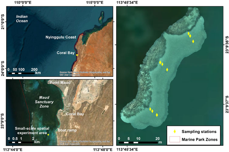
Figure 1. Map of study site. Sampling stations of the soundscape showing the experimental design at Nyinggulu Coast, Western Australia.

2.2 Soundscape sampling

The effect of distance and position of the sensors (underwater acoustic recorders) on the received soundscape was tested using an array of 12 underwater acoustic recorders simultaneously deployed between August 26th–18 September 2022 (Supplementary Table 1). We established three transects (South, Middle, and North) separated by 20 m, at 4 m depth in the sand along the edge of a fringing reef ∼2 m height, ∼500 m length, and ∼110 m width. At each transect we established three sampling stations at varying distances from the reef: 1 m, 2 m, and 5 m (Figure 1; Supplementary Figure 1A). No other reefs or coral heads were located within 100 m. An underwater acoustic recorder was attached to a star-picket (orientation: vertical) at each sampling station, with the hydrophone positioned 60 cm above the seafloor, pointing upwards (Supplementary Figure 1B). Three additional recorders were deployed at each sampling station of the Middle transect using T-bars (orientation: horizontal) positioned on the bottom, pointing to the target reef, with the hydrophone 5 cm above the seafloor (Supplementary Figure 1B). All the instruments were SoundTrap digital sound recorders ST600 (Ocean Instruments). These systems are pistonphone-calibrated at 250 Hz by the manufacturer with a flat response (±3 dB) across its full bandwidth (from 20 Hz to 150 kHz). Recordings were conducted using a 48 kHz sampling frequency, with a duty cycle of 5 min every 15 min, high gain, and the instrument internal clock GPS-synchronized to the local time.

2.3 Soundscape analyses

The recordings were inspected using CHORUS (Gavrilov and Parsons, 2014) in MATLAB^® (The MathWorks Inc., United States). We found no significant contributions of wind sound to the bands of interest during the recording period. We only analysed simultaneous recordings and excluded deployment/retrieval times. Calibrated acoustic data was converted to long-term spectral averages (LTSA, with 2 min averaging period) and power spectral density percentiles with an overlay of the power spectral probability density (PSD%PD). We used the Soundscape Code (SSC) to characterize the amplitude (root-mean-square sound pressure level, $L_{p,rms}$, and peak sound pressure level $L_{p,pk}$), impulsiveness (kurtosis of sound pressure, $\beta$), periodicity within 1 min recordings (time-lagged autocorrelation for 0.1 s mean square sound pressure averages, $Acorr3$), and uniformity (dissimilarity index, $D$) (Wilford et al., 2021); in addition to the acoustic complexity index (ACI). All metrics were computed for the frequency bands containing the main biological contributors to our soundscape (Supplementary Figures 1, 2), fish (200–800 Hz) and invertebrate (2–5 kHz) bands, in MATLAB^® custom code (Azofeifa-Solano et al., 2025) following the original equations (Pieretti et al., 2011; Wilford et al., 2021) with adaptations to terminology (ISO, 2017; Sueur, 2018). The code for the soundscape code metrics is available at MATLAB Central File Exchange (Azofeifa Solano, 2024).

2.4 Statistical analyses

All metrics were assigned to a time of the day according to the specific twilight, sunrise, and sunset time of each day (https://geodesyapps.ga.gov.au). The times of the day were defined as Dawn (beginning of nautical twilight until sunrise), Day (from sunrise until sunset), Dusk (from sunset until end of nautical twilight), and Night (from end of nautical twilight until beginning of following nautical twilight). All analyses were conducted using the R environment, version 4.3.2, in RStudio, version 2024.09.1, (RStudio Team, 2024). Each metric was plotted over time to visualize general patterns. We conducted two different models to test for the influence of distance and orientation of the hydrophones relative to the target habitat on the received soundscape. Time of day was considered by analysing each period separately (Elise et al., 2019). For the distance experiment, we conducted a linear model considering distance from the reef (1 m, 2 m, 5 m) and transect (N: north, M: middle, S: south) as fixed categorical factors. The model residuals were tested to check for normality (Anderson-Darling) and homoscedasticity (Levene). For this comparison we only considered data from the vertical deployments (star-pickets). For the orientation experiment we conducted a linear model considering deployment method (M: middle star-pickets or vertical, T: middle T-bars or horizontal) and distance from the reef (1 m, 2 m, 5 m) as fixed categorical factors, as well as the interactions among them. The model residuals were tested to check for normality (Anderson-Darling) and homoscedasticity (Levene).

3 Results

The soundscape at all the stations shows diel patterns typical of coral reefs, with higher values for the fish band during day, and higher values for the invertebrate band during night (Supplementary Figures 2, 3). All SSC metrics and the $ACI$ showed conspicuous spatial and temporal variability for the fish and the invertebrate bands (Supplementary Figures 4–9). The $L_{p,rms}$, $L_{p,pk}$, $D$, and $ACI$ have noticeable diel patterns, but the $\beta$ and $Acorr3$ did not. Our data had no problems with residual normality or homoscedasticity (Supplementary Table 2).

3.1 Distance experiment

Our results show that for the fish band, only the amplitude (mostly $L_{p,rms}$) varied with distance from the reef (Figure 2), however, the models had a relatively low deviance explained (10% < DE < 50%; Supplementary Tables 3–6). In the case of the invertebrate band, amplitude ($L_{p,rms}$), contrary to our expectations, increased with distance from the reef (Figure 2), with the models explaining most of the variance during dawn and dusk (DE > 50%) (Supplementary Tables 3–6). The remaining metrics did not vary among distances (Supplementary Figures 10–14; Supplementary Tables 3–6).

Figure 2

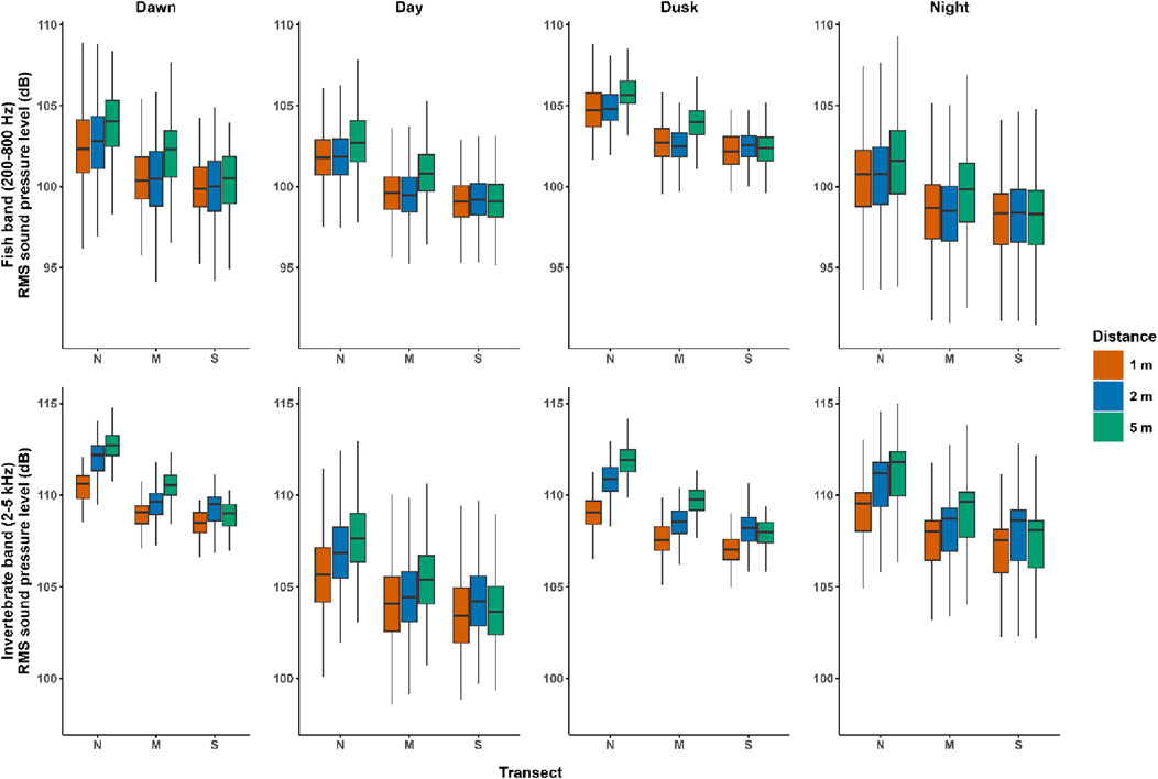
Figure 2. Sound pressure level comparison. Boxplots of root-mean-squared sound pressure level (dB) of the fish band (200 Hz–800 Hz) and the invertebrate band (2 kHz–5 kHz), showing transects and distances from the reef, Nyinggulu Coast, Western Australia. N, north; M, middle; S, south.

3.2 Orientation experiment

We found differences for the fish band metrics between the two deployment methods; however, the models have low deviance explained (DE < 10%; Supplementary Tables 7–10; Figure 3; Supplementary Figures 15–19). In the case of the invertebrate band, the amplitude ($L_{p,rms}$) showed differences between deployment methods during dawn and dusk (Figure 3), with a relatively low deviance (10% < DE < 50%). The amplitude tended to increase with distance from the reef in the vertical deployment, while recordings from the horizontal deployment showed a decreasing amplitude with distance from the reef. The remaining metrics were similar between orientations (Supplementary Figures 15–19).

Figure 3

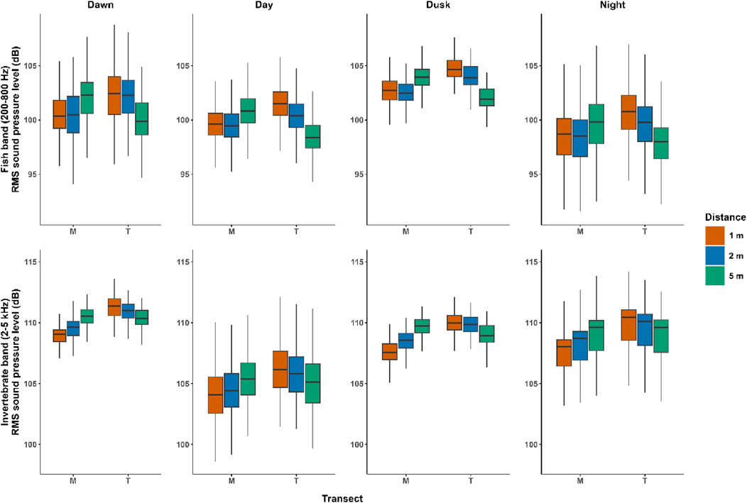
Figure 3. Sound pressure level comparison. Boxplots of root-mean-squared sound pressure level (dB) of the fish band (200 Hz–800 Hz) and the invertebrate band (2 kHz–5 kHz), showing transects (different deployments) and distances from the reef, Nyinggulu Coast, Western Australia. M, middle star-pickets or vertical; T, middle T-bars or horizontal.

4 Discussion

The findings of our experiment clearly indicate that both distance and orientation influence the received soundscape when sampling within shallow coral reefs, which broadly aligns with observations from other habitat types (Urick, 1983; Parsons and Duncan, 2011; Taylor et al., 2024). Here, three main patterns of sound levels were observed: differences among relative distances and orientations of the sensors, differences between frequency bands (fish vs. invertebrate), and differences among times of the day. As it is critical to identify and limit potential sources of bias within soundscape analyses, these results have significant implications for the optimization, testing, validation, and standardization of acoustic sampling methodologies in coastal habitats and in their near field.

We found two distinct patterns in the sound pressure level of the invertebrate band between the sensors pointing upwards (vertical) and those pointing directly at the target habitat (horizontal). In the horizontal deployments, the sound pressure level of the invertebrate band decreased with increasing distance, as predicted (Bies et al., 2023). However, in the vertical deployments, the sound pressure level of the invertebrate band (2–5 kHz) increased slightly with increasing distance, opposite to what would be expected from an incoherent line source (Bies et al., 2023) or even an “extended” sound source area (Radford et al., 2011). We explored potential explanations for this unusual pattern in the invertebrate band. First, we examined pictures from a 3D photogrammetry transect conducted in the same area and time of our study to look for snapping shrimp burrows near to the furthest recorders from the reef. We also scrutinized the LTSA from our recordings to detect loud transient sounds, for example, snaps from snapping shrimp. We discarded this possibility as we found no snapping shrimp burrows located in higher numbers in the sand area 5 m off the reef (Supplementary Figure 20), neither loud transient sound in the LTSAs (Supplementary Figures 2–3). We also explored the potential effect of interference from standing waves in 4 m of water within the near field, considering the phase difference between the direct and reflected sound paths (Urick, 1983; Smith, 2010). Despite some frequencies having minima very close to the position of the hydrophones at 1 m and 2 m off the reef at 60 cm above the seafloor, this is not the case for all frequencies (Supplementary Figure 21). However, our metrics represented an average of sound pressure levels over a wide frequency band (2 kHz–5 kHz), thus, we discarded interference from standing waves as a potential driver of our unusual pattern. Finally, we explored modelling the sound propagation of a hypothetical reef with random sources (snapping shrimp), while randomizing the positions and sound level sources, according to available information (Versluis et al., 2000; Butler et al., 2017; Dinh and Radford, 2021). However, our preliminary models suggested overall declines in sound levels with increasing distance (Supplementary Figure 22), similar to the “extended” sound source area (Radford et al., 2011). The interference between two or more hypothetical sources within an incoherent line source and extended source produce some inhomogeneities in the sound propagation. The seafloor sediment and other environmental variables can influence the sound speed profile; however, our experimental setting is such that the two farthest transects are only separated by 40 m. Thus, it is possible the sediment types and sound speed profiles are similar among these locations. The influence of the seafloor sediment is another further topic future studies might include into consideration. Our three transects, separated only by 20 m, showed the same increasing pattern. This suggests that there might be another explanation for the unusual increasing pattern of sound level.

The hydrophone, or the hydrophone-recorder system, is an important variable to consider when it comes to the received soundscape. A hydrophone’s ability to transform acoustic pressure to an output voltage is called sensitivity, and this is usually characterized for normally incident, quasi-planar acoustic pressure waves as a function of frequency (Saheban and Kordrostami, 2021). However, the sensitivity of a hydrophone also depends on the angle between its acoustic axis and the direction of propagation of the incident wave. The hydrophone directivity describes the difference in output voltage from the quasi-planar acoustic pressure as a function of the angle relative to the hydrophone axis, and it can be represented as a beam pattern (Saheban and Kordrostami, 2021). Previous studies have demonstrated that the hydrophone beam pattern varies according to range, angle, and frequency, with changes of up to 10 dB or 25 dB depending on the seabed (Parsons and Duncan, 2011). For example, Parsons and Duncan (2011) found that the sound level received was lower at higher angles (further off-axis). Similarly, a study on the HydroMoth low-cost underwater recorders discussed the issue of having a hydrophone with direction-dependent sensitivity; and suggested that most commercially available recorders might have some degree of directional bias (Lamont et al., 2022a). Most recorders have a nominally omnidirectional hydrophone extruding from the rest of the cylindrical-shaped recorder to reduce this effect. However, a recent study also found frequency-dependent acoustic directivity on several recorders used in underwater acoustics research: the PVC air-filled Loggerhead Snap, the PVC oil-filled SoundTrap ST300, and the titanium air-filled SoundTrap ST600 (Taylor et al., 2024). Their results indicate that the sensor directivity, which is also frequency-dependent, cannot be neglected, with variations of up to 20 dB as a function of the orientation angle and frequency (Taylor et al., 2024). In the specific case of the SoundTrap ST600 (same model used in this study), the received sound pressure levels drop conspicuously (∼2–10 dB depending on the frequency) at various angles, with increasing losses starting around 90° for 2–5 kHz (Taylor et al., 2025).

In our experimental design, the vertical deployments had the hydrophones pointing upwards, all positioned at 60 cm above the seabed. These hydrophones were located 1 m, 2 m, and 5 m from the edge of the reef. Since only the invertebrate band showed an unexpected pattern, we will focus on the invertebrate sounds. Most invertebrates are found close to the seabed, contrary to the fish which might be expected either close to the seabed or on the water column. Snapping shrimp are the main acoustic contributors to the invertebrate band in coral reefs (Lillis and Mooney, 2018). These shrimp are benthic dwellers and usually hide in borrows or crevices (Knowlton, 1980). Snapping shrimp have an enlarged cheliped with a highly specialized snapping claw (Anker et al., 2006; Kaji et al., 2018). This snapping claw can be closed at a high velocity, displacing water from a socket and producing a cavitation bubble which implodes, resulting in a water jet and a very loud broadband snap sound with peak-to-peak source levels up to 183–189 dB re 1 μPa at 1 m (Au and Banks, 1998; Versluis et al., 2000; Dinh and Radford, 2021). Let us consider a hypothetical snapping shrimp at seabed at the edge of the reef which produces a snap. Now, consider the angles between the direct propagation path of this snap sound and the acoustic axis of the hydrophones located 1 m, 2 m, and 5 m from the shrimp and at 60 cm height from the seabed. These angles are approximately 130°, 116°, and 106°, respectively (Supplementary Figure 23). Considering the directional response results of the SoundTrap ST600 (Taylor et al., 2025), in the specific case of a sound source (i.e., snapping shrimp) located on the seabed, the sensitivity of the hydrophone as a function of the angle will result in lower sound levels at the recorder located closer to the snapping shrimp (higher angles), and higher levels with increasing distance (lower angles) (Supplementary Figure 23). Thus, the unexpected pattern of the sound pressure levels of the invertebrate band for the vertical instruments in our study could be related to the sensor directivity, and the angles formed between the direct path of the wave and the acoustic axis of the hydrophones.

Our results have significant implications for underwater acoustics in coastal habitats and instruments deployed in the near field of the target habitats or species. Further studies must address the potential effects of the relative distance and orientation of the sensors and the sound sources of interest. For example, methodologies should be developed to quantify and minimize any potential methodological bias introduced by the spatial array of sensors according to the target sound sources and the sound propagation in the ecosystem.

We observed two different patterns in the received sound pressure level between the fish band (200–800 Hz) and invertebrate band (2–5 kHz). Significant differences among distances and orientations were detected in the invertebrate band, but the pattern for fish was not obvious and our models provided low explained variation. Sound propagation models consider the effect of different wavelengths of sound and its interaction with boundaries and other inhomogeneities (Oliveira et al., 2021). Previous studies have also observed that attenuation patterns differ between the fish and invertebrate frequency bands (Radford et al., 2011; Piercy et al., 2014; Raick et al., 2021). For example, a study in Hawai’i found that invertebrate frequencies attenuate rapidly beyond 200 m from the reef compared to fish frequencies, which might be expected as sound attenuation in sea water is more pronounced at higher frequencies (Kaplan and Mooney, 2016). However, the effect of absorption in sea water is considered to be negligible in the range of frequencies and the distances of our study (Ainslie and McColm, 1998); therefore, other, more complex and site-specific propagation effects such as multiple bottom and surface reflections and scattering are the likely cause of this observed rapid attenuation.

Differences among distances and orientations were more evident during dawn and dusk for both fish and invertebrate bands. Dawn and dusk have significantly higher (i.e., >30 dB above background levels) sound activity for fish and invertebrate in coral reefs (Staaterman et al., 2014; McWilliam et al., 2017). In some cases, however, the higher variability of vocalizations at dawn and dusk might obscure other ecological patterns and it is not recommended to use these times for inter-sample comparisons (Elise et al., 2019). The marked differences found at twilight periods might be explained by the overall higher sound production, with declines that are more noticeable with distance. Otherwise, the lower levels during day and night could result in less noticeable dependence on range from the reef. Similarly, in Hawai’i, the sound attenuation was more conspicuous during dawn than during mid-morning than other times of the day (Kaplan and Mooney, 2016).

4.1 Implications

Ocean soundscapes convey valuable information about ecological processes (Duarte et al., 2021) and represent a possible solution for large-scale monitoring (Gibb et al., 2019). Acoustic sampling and analyses still require validation (Mooney et al., 2020). If we aim to produce reliable acoustic data to study and monitor our oceans, we must develop practices that avoid or reduce methodological biases. Future studies should consider the significance of field-testing sensor directivity to quantify and minimize any possible methodological bias on the received soundscape. Biased source levels as functions of angles, distances, and frequencies would have significant implications for a number of acoustic studies. For example, these biases might hamper localization methods that rely on the received acoustic energy from multiple sensors if the variation in the beam pattern is not considered (Parsons and Duncan, 2011).

Another example is ecoacoustics, which commonly use acoustic indices to summarize and characterize soundscapes (Sueur et al., 2014; Gibb et al., 2019). For example, the acoustic complexity index quantifies the variability of the sound signal within each frequency band over time (Pieretti et al., 2011). Likewise, many of these indices extract information from the spectrogram, which is a representation of acoustic power as a function time and frequency (Sueur, 2018). However, these methods rely on the assumption that the received soundscape is a function of the ecosystem and not an artifact of methodological bias. If the frequency-dependent directivity of the hydrophone is not addressed (Parsons and Duncan, 2011; Taylor et al., 2024), the recorded soundscape will not be representative of the true soundscape, as the acoustic energy of some frequencies will be differentially affected. Thus, we must consider the directivity of the hydrophones during the processing of the data.

Soundscapes have an important role for orientation in a range of marine species (Simpson et al., 2005; Lillis et al., 2018a), and are the foundation of the ecological application of soundscape analyses (Duarte et al., 2021). Animals can extract information from the soundscape to interact with their surrounding environment (Dall et al., 2005; Deichmann et al., 2018; Duarte et al., 2021). In coral reefs, for example, acoustic cues play an important role for navigation towards suitable habitats and settle-decision in many marine species (Tolimieri et al., 2004; Simpson et al., 2005; Montgomery et al., 2006; Vermeij et al., 2010; Lillis et al., 2018a). It is important to consider that the perception of sounds of marine animals depends on the energy of each source, the direction of the propagation of the signals, the influence of the physical environment on the propagation of the signals, the behavioural and historical context of the listener, and the hearing capabilities of the listener (Miksis-Olds et al., 2018). Thus, considering the propagation of sound and the directivity of the listener (sensor or animal) might help us elucidate the ecological importance of sounds, and how sources and listeners in the environment might perceive and respond to the acoustic signals.

Data availability statement

The raw data supporting the conclusions of this article will be made available by the authors, without undue reservation.

Author contributions

JA-S: Conceptualization, Data curation, Formal Analysis, Investigation, Methodology, Software, Visualization, Writing–original draft, Writing–review and editing. CE: Formal Analysis, Software, Supervision, Validation, Writing–review and editing. CT: Formal Analysis, Software, Validation, Visualization, Writing–review and editing. RM: Supervision, Writing–review and editing. RB: Project administration, Resources, Supervision, Writing–review and editing. DP: Data curation, Formal Analysis, Methodology, Visualization, Writing–review and editing. MP: Conceptualization, Formal Analysis, Investigation, Methodology, Supervision, Writing–review and editing.

Funding

The author(s) declare that financial support was received for the research, authorship, and/or publication of this article. This research was funded by the BHP–AIMS Australian Coral Reef Resilience Initiative. JCAS was supported by Curtin University in the form of a Curtin Strategic Scholarship and by BHP–AIMS in the form of a Top-Up Scholarship. ACRRI is jointly funded by BHP and the Australian Institute of Marine Science.

Acknowledgments

We acknowledge the Baiyungu, Thalanyji and Yinikurtura People as the Traditional Owners of the Nyinggulu Coast where this research occurs. We pay our respects to these first nations people, their elders past, present and emerging and acknowledge their continuing spiritual connection to their land and sea country. The authors acknowledge the support of the Australian Coral Reef Resilience Initiative (ACRRI) in the field data collection. We are thankful to the support of Mark Meekan, Anthon Kuret, Matt Birtt, Alec Duncan, and the staff of Coral Bay Research Station–Murdoch University.

Conflict of interest

The authors declare that the research was conducted in the absence of any commercial or financial relationships that could be construed as a potential conflict of interest.

Generative AI statement

The authors declare that no Generative AI was used in the creation of this manuscript.

Publisher’s note

All claims expressed in this article are solely those of the authors and do not necessarily represent those of their affiliated organizations, or those of the publisher, the editors and the reviewers. Any product that may be evaluated in this article, or claim that may be made by its manufacturer, is not guaranteed or endorsed by the publisher.

Supplementary material

The Supplementary Material for this article can be found online at: https://www.frontiersin.org/articles/10.3389/frsen.2025.1527988/full#supplementary-material

References

Ainslie, M. A., and McColm, J. G. (1998). A simplified formula for viscous and chemical absorption in sea water. J. Acoust. Soc. Am. 103 (3), 1671–1672. doi:10.1121/1.421258

CrossRef Full Text | Google Scholar

Anker, A., Ahyong, S. T., Noël, P. Y., and Palmer, A. R. (2006). Morphological phylogeny of alpheid shrimps: parallel preadaptation and the origin of a key morphological innovation, the snapping claw. Evolution 60, 2507–2528. doi:10.1111/j.0014-3820.2006.tb01886.x

PubMed Abstract | CrossRef Full Text | Google Scholar

Au, W. W. L., and Banks, K. (1998). The acoustics of the snapping shrimp Synalpheus parneomeris in Kaneohe Bay. J. Acoust. Soc. Am. 103(1), 41–47. doi:10.1121/1.423234

CrossRef Full Text | Google Scholar

Azofeifa Solano, J. C. (2024). SSCmetrics: a MATLAB tool to compute the Soundscape Code. Version 1.0.2.

Google Scholar

Azofeifa-Solano, J. C., Parsons, J. G. M., Brooker, R., McCauley, R., Pygas, D., Feeney, W., et al. (2025). Soundscape analysis reveals fine ecological differences among coral reefs habitats. Ecol. Indic.

Google Scholar

Bies, D. A., Hansen, C. H., Howard, C. Q., and Hansen, K. L. (2023). Engineering noise control. Boca Raton: CRC Press.

Google Scholar

Butler, J., Butler IV, M. J., and Gaff, H. (2017). Snap, crackle, and pop: acoustic-based model estimation of snapping shrimp populations in healthy and degraded hard-bottom habitats. Ecol. Indic. 77, 377–385. doi:10.1016/j.ecolind.2017.02.041

CrossRef Full Text | Google Scholar

Dall, S. R. X., Giraldeau, L. A., Olsson, O., McNamara, J. M., and Stephens, D. W. (2005). Information and its use by animals in evolutionary ecology. Trends Ecol. and Evol. 20 (4), 187–193. doi:10.1016/j.tree.2005.01.010

PubMed Abstract | CrossRef Full Text | Google Scholar

Deichmann, J. L., Acevedo-Charry, O., Barclay, L., Burivalova, Z., Campos-Cerqueira, M., d'Horta, F., et al. (2018). It's time to listen: there is much to be learned from the sounds of tropical ecosystems. Biotropica 50 (5), 713–718. doi:10.1111/btp.12593

CrossRef Full Text | Google Scholar

Dimoff, S. A., Halliday, W. D., Pine, M. K., Tietjen, K. L., Juanes, F., and Baum, J. K. (2021). The utility of different acoustic indicators to describe biological sounds of a coral reef soundscape. Ecol. Indic. 124, 107435. doi:10.1016/j.ecolind.2021.107435

CrossRef Full Text | Google Scholar

Dinh, J. P., and Radford, C. (2021). Acoustic particle motion detection in the snapping shrimp (Alpheus richardsoni). J. Comp. Physiology a-Neuroethology Sens. Neural Behav. Physiology 207 (5), 641–655. doi:10.1007/s00359-021-01503-4

PubMed Abstract | CrossRef Full Text | Google Scholar

Duarte, C. M., Chapuis, L., Collin, S. P., Costa, D. P., Devassy, R. P., Eguiluz, V. M., et al. (2021). The soundscape of the Anthropocene ocean. Science 371 (6529), eaba4658. doi:10.1126/science.aba4658

PubMed Abstract | CrossRef Full Text | Google Scholar

Elise, S., Bailly, A., Urbina-Barreto, I., Mou-Tham, G., Chiroleu, F., Vigliola, L., et al. (2019). An optimised passive acoustic sampling scheme to discriminate among coral reefs’ ecological states. Ecol. Indic. 107, 105627. doi:10.1016/j.ecolind.2019.105627

CrossRef Full Text | Google Scholar

Elise, S., Guilhaumon, F., Mou-Tham, G., Urbina-Barreto, I., Vigliola, L., Kulbicki, M., et al. (2022). Combining passive acoustics and environmental data for scaling up ecosystem monitoring: a test on coral reef fishes. Remote Sens. 14 (10), 2394. doi:10.3390/rs14102394

CrossRef Full Text | Google Scholar

Gavrilov, A. N., and Parsons, M. J. G. (2014). A matlab tool for the characterisation of recorded underwater sound (chorus). Acoust. Aust. 42 (3), 190–196.

Google Scholar

Gibb, R., Browning, E., Glover-Kapfer, P., and Jones, K. E. (2019). Emerging opportunities and challenges for passive acoustics in ecological assessment and monitoring. Methods Ecol. Evol. 10, 169–185. doi:10.1111/2041-210x.13101

CrossRef Full Text | Google Scholar

Gilmour, J. P., Cook, K. L., Ryan, N. M., Puotinen, M. L., Green, R. H., Shedrawi, G., et al. (2019). The state of Western Australia's coral reefs. Coral Reefs 38 (4), 651–667. doi:10.1007/s00338-019-01795-8

CrossRef Full Text | Google Scholar

Hearn, C. J., Hatcher, B. G., Masini, R. J., and Simpson, C. J. (1986). Oceanographic processes on the Ningaloo coral reef. Perth: Centre for Water Research, University of Western Australia. Environmental dynamics report ED-86-171.

Google Scholar

ISO (2017). 18405.2. Underwater acoustics—terminology. Geneva: International Organization for Standardization.

Google Scholar

Jones, I. T., Gray, M. D., and Mooney, T. A. (2022). Soundscapes as heard by invertebrates and fishes: particle motion measurements on coral reefs. J. Acoust. Soc. Am. 152 (1), 399–415. doi:10.1121/10.0012579

PubMed Abstract | CrossRef Full Text | Google Scholar

Kaji, T., Anker, A., Wirkner, C. S., and Palmer, A. R. (2018). Parallel saltational evolution of ultrafast movements in snapping shrimp claws. Curr. Biol. 28, 106–113.e4. doi:10.1016/j.cub.2017.11.044

PubMed Abstract | CrossRef Full Text | Google Scholar

Kaplan, M. B., and Mooney, T. A. (2016). Coral reef soundscapes may not be detectable far from the reef. Sci. Rep. 6, 31862. doi:10.1038/srep31862

PubMed Abstract | CrossRef Full Text | Google Scholar

Kaplan, M. B., Mooney, T. A., Partan, J., and Solow, A. R. (2015). Coral reef species assemblages are associated with ambient soundscapes. Mar. Ecol. Prog. Ser. 533, 93–107. doi:10.3354/meps11382

CrossRef Full Text | Google Scholar

Knowlton, N. (1980). Sexual selection and dimorphism in two demes of a symbiotic, pair-bonding snapping shrimp. Evolution 34 (1), 161–173. doi:10.2307/2408325

PubMed Abstract | CrossRef Full Text | Google Scholar

Lamont, T. A. C., Chapuis, L., Williams, B., Dines, S., Gridley, T., Frainer, G., et al. (2022a). HydroMoth: testing a prototype low-cost acoustic recorder for aquatic environments. Remote Sens. Ecol. Conservation 8, 362–378. doi:10.1002/rse2.249

CrossRef Full Text | Google Scholar

Lamont, T. A. C., Williams, B., Chapuis, L., Prasetya, M. E., Seraphim, M. J., Harding, H. R., et al. (2022b). The sound of recovery: coral reef restoration success is detectable in the soundscape. J. Appl. Ecol. 59 (3), 742–756. doi:10.1111/1365-2664.14089

CrossRef Full Text | Google Scholar

Larsen, O. N., and Radford, C. (2018). “Acoustic conditions affecting sound communication in air and underwater,” in Effects of anthropogenic noise on animals. Editors H. Slabbekoorn, R. Dooling, A. Popper, and R. Fay (New York: Springer), 109–144.

Google Scholar

Lillis, A., Apprill, A., Armenteros, M., and Mooney, T. A. (2023). “Small-scale variation in the soundscapes of coral reefs,” in The effects of noise on aquatic life. Editors A. N. Popper, J. Sisneros, A. D. Hawkins, and F. Thomsen (Cham: Springer), 1–15.

CrossRef Full Text | Google Scholar

Lillis, A., Apprill, A., Suca, J. J., Becker, C., Llopiz, J. K., and Mooney, T. A. (2018a). Soundscapes influence the settlement of the common Caribbean coral Porites astreoides irrespective of light conditions. R. Soc. Open Sci. 5 (12), 181358. doi:10.1098/rsos.181358

PubMed Abstract | CrossRef Full Text | Google Scholar

Lillis, A., Caruso, F., Mooney, T. A., Llopiz, J., Bohnenstiehl, D., and Eggleston, D. B. (2018b). Drifting hydrophones as an ecologically meaningful approach to underwater soundscape measurement in coastal benthic habitats. J. Ecoacoustics 2 (1), 1. doi:10.22261/JEA.STBDH1

CrossRef Full Text | Google Scholar

Lillis, A., and Mooney, T. A. (2018). Snapping shrimp sound production patterns on Caribbean coral reefs: relationships with celestial cycles and environmental variables. Coral Reefs 37 (2), 597–607. doi:10.1007/s00338-018-1684-z

CrossRef Full Text | Google Scholar

Lin, M., and Yang, C. (2020). Ocean observation technologies: a review. Chin. J. Mech. Eng. 33 (1), 32–18. doi:10.1186/s10033-020-00449-z

CrossRef Full Text | Google Scholar

Lin, T. H., Akamatsu, T., Sinniger, F., and Harii, S. (2021). Exploring coral reef biodiversity via underwater soundscapes. Biol. Conserv. 253, 108901. doi:10.1016/j.biocon.2020.108901

CrossRef Full Text | Google Scholar

McCauley, R. D., and Cato, D. H. (2000). Patterns of fish calling in a nearshore environment in the Great Barrier Reef. Philosophical Trans. R. Soc. Lond. Ser. B-Biological Sci. 355 (1401), 1289–1293. doi:10.1098/rstb.2000.0686

PubMed Abstract | CrossRef Full Text | Google Scholar

McCauley, R. D., Meekan, M. G., and Parsons, M. J. (2021). Acoustic pressure, particle motion, and induced ground motion signals from a commercial seismic survey array and potential implications for environmental monitoring. J. Mar. Sci. Eng. 9 (6), 571. doi:10.3390/jmse9060571

CrossRef Full Text | Google Scholar

McWilliam, J. N., McCauley, R. D., Erbe, C., and Parsons, M. J. G. (2017). Patterns of biophonic periodicity on coral reefs in the Great Barrier Reef. Sci. Rep. 7, 17459. doi:10.1038/s41598-017-15838-z

PubMed Abstract | CrossRef Full Text | Google Scholar

Meyer, E., and Neumann, E. G. (1972). Physical and applied acoustics: an introduction. Academic Press.

Google Scholar

Miksis-Olds, J. L., Martin, B., and Tyack, P. L. (2018). Exploring the ocean through soundscapes. Acoust. Today 14 (9), 26–34.

Google Scholar

Montgomery, J. C., Jeffs, A., Simpson, S. D., Meekan, M., and Tindle, C. (2006). Sound as an orientation cue for the pelagic larvae of reef fishes and decapod crustaceans. Adv. Mar. Biol. 51, 143–196. doi:10.1016/S0065-2881(06)51003-X

PubMed Abstract | CrossRef Full Text | Google Scholar

Mooney, T. A., Di Iorio, L., Lammers, M., Lin, T. H., Nedelec, S. L., Parsons, M., et al. (2020). Listening forward: approaching marine biodiversity assessments using acoustic methods. R. Soc. Open Sci. 7 (8), 201287. doi:10.1098/rsos.201287

PubMed Abstract | CrossRef Full Text | Google Scholar

Mumby, P. J., Broad, K., Brumbaugh, D. R., Dahlgren, C. P., Harborne, A. R., Hastings, A., et al. (2008). Coral reef habitats as surrogates of species, ecological functions, and ecosystem services. Conserv. Biol. 22 (4), 941–951. doi:10.1111/j.1523-1739.2008.00933.x

PubMed Abstract | CrossRef Full Text | Google Scholar

Obura, D. O., Aeby, G., Amornthammarong, N., Appeltans, W., Bax, N., Bishop, J., et al. (2019). Coral reef monitoring, reef assessment technologies, and ecosystem-based management. Front. Mar. Sci. 6, 580. doi:10.3389/fmars.2019.00580

CrossRef Full Text | Google Scholar

O'Connor, B., Bojinski, S., Röösli, C., and Schaepman, M. E. (2020). Monitoring global changes in biodiversity and climate essential as ecological crisis intensifies. Ecol. Inf. 55, 101033. doi:10.1016/j.ecoinf.2019.101033

CrossRef Full Text | Google Scholar

Oliveira, T. C., Lin, Y. T., and Porter, M. B. (2021). Underwater sound propagation modeling in a complex shallow water environment. Front. Mar. Sci. 8, 751327. doi:10.3389/fmars.2021.751327

CrossRef Full Text | Google Scholar

Parsons, M. J. G., and Duncan, A. J. (2011). The effect of seabed properties on the receive beam pattern of hydrophone located on the seafloor. Acoust. Aust. 39 (3), 106–112.

Google Scholar

Pereira, H. M., and Cooper, H. D. (2006). Towards the global monitoring of biodiversity change. Trends Ecol. and Evol. 21 (3), 123–129. doi:10.1016/j.tree.2005.10.015

CrossRef Full Text | Google Scholar

Piercy, J. J. B., Codling, E. A., Hill, A. J., Smith, D. J., and Simpson, S. D. (2014). Habitat quality affects sound production and likely distance of detection on coral reefs. Mar. Ecol. Prog. Ser. 516, 35–47. doi:10.3354/meps10986

CrossRef Full Text | Google Scholar

Pieretti, N., Farina, A., and Morri, D. (2011). A new methodology to infer the singing activity of an avian community: the Acoustic Complexity Index (ACI). Ecol. Indic. 11 (3), 868–873. doi:10.1016/j.ecolind.2010.11.005

CrossRef Full Text | Google Scholar

Radford, C. A., Tindle, C. T., Montgomery, J. C., and Jeffs, A. G. (2011). Modelling a reef as an extended sound source increases the predicted range at which reef noise may be heard by fish larvae. Mar. Ecol. Prog. Ser. 438, 167–174. doi:10.3354/meps09312

CrossRef Full Text | Google Scholar

Raick, X., Di Iorio, L., Gervaise, C., Lossent, J., Lecchini, D., and Parmentier, E. (2021). From the reef to the ocean: revealing the acoustic range of the biophony of a coral reef (moorea island, French polynesia). J. Mar. Sci. Eng. 9 (4), 420. doi:10.3390/jmse9040420

CrossRef Full Text | Google Scholar

RStudio Team (2024). RStudio: integrated development for R. Boston: RStudio, PBC. Version 2024.09.1.

Google Scholar

Saheban, H., and Kordrostami, Z. (2021). Hydrophones, fundamental features, design considerations, and various structures: a review. Sensors Actuators A Phys. 329, 112790. doi:10.1016/j.sna.2021.112790

CrossRef Full Text | Google Scholar

Sethi, S. S., Ewers, R. M., Jones, N. S., Orme, C. D. L., and Picinali, L. (2018). Robust, real-time and autonomous monitoring of ecosystems with an open, low-cost, networked device. Methods Ecol. Evol. 9 (12), 2383–2387. doi:10.1111/2041-210X.13089

CrossRef Full Text | Google Scholar

Simpson, C. J., Cary, J. L., and Masini, R. J. (1993). Destruction of corals and other reef animals by coral spawn slicks on Ningaloo Reef, Western Australia. Coral Reefs 12 (3), 185–191. doi:10.1007/bf00334478

CrossRef Full Text | Google Scholar

Simpson, S. D., Meekan, M., Montgomery, J., McCauley, R., and Jeffs, A. (2005). Homeward sound. Science 308 (5719), 221. doi:10.1126/science.1107406

PubMed Abstract | CrossRef Full Text | Google Scholar

Smith, W. F. (2010). Waves and oscillations: a prelude to quantum mechanics. Oxford University Press.

Google Scholar

Staaterman, E., Paris, C. B., DeFerrari, H. A., Mann, D. A., Rice, A. N., and D'Alessandro, E. K. (2014). Celestial patterns in marine soundscapes. Mar. Ecol. Prog. Ser. 508, 17–32. doi:10.3354/meps10911

CrossRef Full Text | Google Scholar

Staaterman, E., Rice, A. N., Mann, D. A., and Paris, C. B. (2013). Soundscapes from a tropical eastern pacific reef and a caribbean sea reef. Coral Reefs 32 (2), 553–557. doi:10.1007/s00338-012-1007-8

CrossRef Full Text | Google Scholar

Sueur, J. (2018). Sound analysis and synthesis with R. Cham: Springer.

Google Scholar

Sueur, J., Farina, A., Gasc, A., Pieretti, N., and Pavoine, S. (2014). Acoustic indices for biodiversity assessment and landscape investigation. Acta Acustica united Acustica 100 (4), 772–781. doi:10.3813/AAA.918757

CrossRef Full Text | Google Scholar

Tallis, H., Guerry, A., and Daily, G. C. (2013). “Ecosystem services,” in Ecological systems (New York: Springer).

Google Scholar

Taylor, R. T., Ballard, M., Cushing, C. W., Wilson, P. S., Lee, K. M., McNeese, A. R., et al. (2024). Evaluating the directivity of compact underwater acoustic recording devices. J. Acoust. Soc. Am. 155 (3), A343–A344. doi:10.1121/10.0027766

CrossRef Full Text | Google Scholar

Taylor, R. T., Ballard, M. S., Cushing, C. W., Lee, K. M., McNeese, A. R., Wilson, P. S., et al. (2025). “Evaluating the directivity of compact underwater acoustic recording devices,” in Proceedings of meetings on acoustics.

Google Scholar

Thomson, D. P., Babcock, R. C., Haywood, M. D., Vanderklift, M. A., Pillans, R. D., Bessey, C., et al. (2020). Zone specific trends in coral cover, genera and growth-forms in the World-Heritage listed Ningaloo Reef. Mar. Environ. Res. 160, 105020. doi:10.1016/j.marenvres.2020.105020

PubMed Abstract | CrossRef Full Text | Google Scholar

Tolimieri, N., Haine, O., Jeffs, A., McCauley, R., and Montgomery, J. (2004). Directional orientation of pomacentrid larvae to ambient reef sound. Coral Reefs 23 (2), 184–191. doi:10.1007/s00338-004-0383-0

CrossRef Full Text | Google Scholar

Tyack, P. L., Akamatsu, T., Boebel, O., Chapuis, L., Debusschere, E., de Jong, C., et al. (2023). “Ocean sound essential ocean variable implementation plan,” in International quiet ocean experiment, scientific committee on oceanic research and partnership for observation of the Global Ocean.

Google Scholar

Urick, R. J. (1983). Principles of underwater sound. New York: MacGraw-Hill.

Google Scholar

Vermeij, M. J. A., Marhaver, K. L., Huijbers, C. M., Nagelkerken, I., and Simpson, S. D. (2010). Coral larvae move toward reef sounds. Plos One 5 (5), e10660. doi:10.1371/journal.pone.0010660

PubMed Abstract | CrossRef Full Text | Google Scholar

Versluis, M., Schmitz, B., von der Heydt, A., and Lohse, D. (2000). How snapping shrimp snap: through cavitating bubbles. Science 289(5487), 2114–2117. doi:10.1126/science.289.5487.2114

PubMed Abstract | CrossRef Full Text | Google Scholar

Wilford, D. C., Miksis-Olds, J. L., Martin, S. B., Howard, D. R., Lowell, K., Lyons, A. P., et al. (2021). Quantitative soundscape analysis to understand multidimensional features. Front. Mar. Sci. 8, 672336. doi:10.3389/fmars.2021.672336

CrossRef Full Text | Google Scholar

Wood, S. N. (2011). Fast stable restricted maximum likelihood and marginal likelihood estimation of semiparametric generalized linear models. J. R. Stat. Soc. Ser. B Stat. Methodol. 73, 3–36. doi:10.1111/j.1467-9868.2010.00749.x

CrossRef Full Text | Google Scholar