Application of high-precision terrestrial light detection and ranging to determine the dislocation geomorphology of Yumen Fault, China

Ground-based three-dimensional (3D) light detection and ranging (LiDAR) is used to collect high-density point clouds of terrain for high-precision topographic survey, remove information on surface vegetation, and allow for the study of fault rupture. Selected as the study area was the west side of the Yumen Fault in China, characterized by a thrust nappe, and information on this typical fault landform. Fundamental issues such as ground-based 3D LiDAR for field collection, data processing, and 3D fault modeling were then analyzed. Finally, the high-precision topography of the surface rupture in this area was obtained, revealing the typical dextral strike–slip dislocation along the fault zone. In the process of data processing, the iterative closet point (ICP) and the optimal point cloud density were used to improve the high efficiency and precision of data processing. Finally, based on point cloud data processing, a digital elevation model (DEM) with a spatial resolution of 0.1 m was obtained for the study area to classify the geomorphic unit, obtain information on the fault scarp and fault broken gully terrain, and quantitatively study and analyze the horizontal dislocation of gully and displacement distance of the fault scarp. This process revealed several seismic events along the fault zone, accompanied by a typical dextral strike–slip phenomenon.

1 Introduction

In recent years, there has been rapid advances in remote sensing technology, giving it the ability to capture the geological structure at a macro level. This is why it is increasingly applied in the quantitative study of active faults (He, 2011; Klinger et al., 2011; Bello et al., 2022, Bello et al., 2021; Crosby et al., 2020). However, remote sensing satellite images are affected by resolution, so they cannot meet the requirements of the minor geomorphologic changes of active faults. The development of high-resolution topography technologies allows for the rapid acquisition of high-precision topographic and geomorphic data (Jiang et al., 2018; Bi et al., 2011; Wang et al., 2018), such as light detection and ranging (LiDAR) (Carter et al., 2007; Haddad et al., 2012; Baran et al., 2010; Chen et al., 2014; Liu et al., 2013; Ren et al., 2014; Jiang et al., 2017; Xu et al., 2022) and unmanned aerial vehicles (UAV) (Jiao et al., 2016a; Uysal et al., 2015; Cirillo et al., 2022). Tape measures, flatbed plotters, and total stations are the most commonly used instruments in traditional topographic and geomorphic survey, and these measurements can be performed on a single point or within a small range at sub-meter accuracy. However, these methods are limited by the need for manual operation and low efficiency. The rapid development of measurement technology has led to the gradual evolution of topographic and geomorphic measurement technology from the traditional total station to the present real time kinematic (RTK) (Cirillo et al., 2022); the efficiency and precision of the three-dimensional (3D) LiDAR (Baran et al., 2010; Jiang et al., 2017; Xu et al., 2022), UAVs (Baran et al., 2010; Jiao et al., 2016a; Cirillo et al., 2022; Westoby et al., 2012; Johnson et al., 2014), and other measuring methods have been improved significantly. The LiDAR scanning system is a type of optical remote sensing technology. In contrast with radio waves emitted by traditional radar, the LiDAR scanning system collects the surface information of the target according to the optical signal. LiDAR is a remote sensing system for active detection; it transmits laser pulses to the surface of the object to be measured and processes the optical signal to determine the features of the object. It can record relevant information during measurement in real time, such as the scanning angle, distance, and point coordinates.

Many scholars and geoscientists have applied LiDAR technology in the field of earth science (Zielke et al., 2010; Wechsler et al., 2009; Zielke and Arrowsmith, 2012; Zhou et al., 2013; Johnson et al., 2014; Zielke et al., 2015). Based on LiDAR technology, Harding and Berghoff (2000) collected high-density point cloud data on the geomorphology of the Seattle fault and carried out fine fault mapping, from which they identified numerous new fault scarps and provided a basis for the site selection of a subsequent exploratory trough. Hudnut (2002) used airborne LiDAR technology to collect point cloud data along the surface rupture zone after the Hector Mine earthquake to obtain high-resolution topographic profile information on this region, thus allowing for the estimation of the coseismic displacement of the earthquake. Hilley and Arrowsmith, (2008) used LiDAR to collect point cloud data on the San Andreas fault and studied the relationship between the basin relief and river steepness coefficient. Furthermore, they used LiDAR data to carry out geomorphic and hydrological analysis, thus identifying tectonic geomorphic evolution at different time intervals. Begg and Mouslopoulou (2010) conducted airborne LiDAR point cloud data collection on the Toupo rift zone in New Zealand and identified 122 traces of active fault zones. Chen et al. (2014) and Liu et al. (2013) carried out an airborne LiDAR scanning survey on 127 km of the Haiyuan Fault and studied the active faulting and topography, respectively. Jiao et al. (2016b) used ground-based LiDAR to collect fine point cloud data at Bailu Middle School after the Wenchuan earthquake and studied and analyzed the buildings and terrain scarp area. Jiang et al. (2017) used ground-based LiDAR and high-resolution images to study and analyze the slip rate and recurrence interval on the Lenglongling fault.

In China, airborne and ground-based LiDAR are the most common applications of LiDAR technology. Compared with airborne LiDAR, ground-based LiDAR has the advantages of low cost, convenient operation, and meets the needs of many researchers. So, in this study, surface faulting in Xigou Ore on the western side of Yumen Fault Zone was selected for the application of ground-based LiDAR measurement technology to study active faults, and a comprehensive operation process of LiDAR, including field measurement (instrument frame station, site distribution) and data processing (point cloud filtering, registration, compression, interpolation modeling) was performed. The high-precision topographic and geomorphic data obtained were used to analyze the typical geomorphic features of Yumen Fault Zone for quantitative research and analysis.

2 Geological setting

Yumen Fault is an active fault that developed from the Qilian Mountains in the southern boundary of the Jiuxi Basin. However, for the northern margin of the Qinghai–Tibet Plateau, the Yumen Fault is also the most nascent fold-and-thrust due to the influence of the northward expansion mode of the Qinghai–Tibet Plateau (Chen et al., 2008; Ran et al., 2013; Li et al., 2016). The Yumen Fault is approximately 130-km long, with an overall WNW strike and S-vergence. It features a thrust nappe and is composed of an east and a west section. The Yumen Fault covers a unique tectonic position: it is connected with the Altyn Fault on the west side and forms a significant section of the northern Qilian Mountain Fault Zone (Figure 1). Therefore, the Yumen Fault is affected by the northern Qilian Mountain Thrust Fault and the Altyn Fault on the west side (Ran et al., 2013; Li et al., 2016). The Yumen, Hanxia-Dahuanggou, and Fodongmiao faults jointly form the nappe structural belt in the western part of the northern margin of Qilian Mountain, and they are distributed in the right row. The Yumen Fault is considered to have been active during the Holocene and was responsible for the Yumen earthquake in 2002 (Li et al., 2016; Liu et al., 2024); some scholars and geoscientists speculate that there were four paleoearthquakes in the Yumen Fault (Li et al., 2016; Min et al., 2002). Xiang et al. (1990), Min et al. (2002), and Li et al. (2016) assent consistens with the huge thrust napper on Yumen Fault, but the existence and direction of horizontal displacement are controversial. Some argue that the Yumen Fault has thrust but lacks a horizontal strike–slip component (Xiang and Guo, 1990), while others believe it has a right-lateral horizontal displacement in the early stage and an obvious left-lateral horizontal component in the late stage (Li et al., 2016; Min et al., 2002).

Figure 1

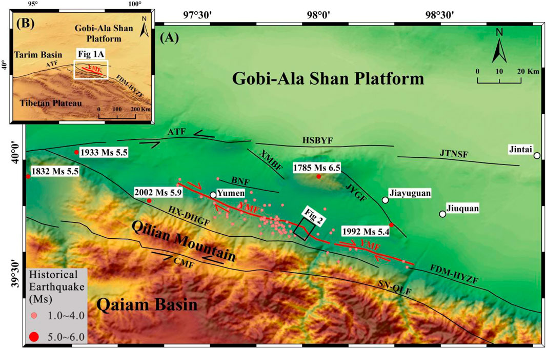
Figure 1. Geological setting of the Yumen Fault (YMF). (A) Red line highlights YMF. Black lines show the distribution of the surrounding major faults: ATF, Altun Tagh Fault; HSBYE, Heishanbeiyuan Fault; JTNSF, Jintananshan Fault; XMBF, Xinminbao Fault; BNF, Bainanshan Fault; JYGF, Jiayuguan Fault; HX-DHGF, Hanxia–Dahuagngou Fault; FDM-HYZF, Fodongmiao–Hongyazi Fault; CMF, Changma Fault; SN-QLF, Sunan–Qilian Fault (faults are Deng et al., 2002). Red dots along YMF indicate historical and instrumental earthquake. (B) Inset shows the location of Panel (A) in the northeastern Tibetan Plateau. White rectangle shows the location of Panel (A) along YMF.

3 Data acquisition and processing

Using high-resolution topographic remote sensing images and high-precision topographic data, tectonic geomorphic dislocation can be constrained, fault rupture history restored, and paleoseismic events identified. Based on this, the distribution characteristics of seismic displacement and the fault rupture mode can be defined, and the recurrence cycle of strong earthquakes can be estimated. Therefore, ground-based LiDAR was used in this study to conduct high-density point clouds in a typical surface rupture zone in the western section of Yumen Fault. The topography of this area is relatively complex. To ensure that the collected point-cloud data can adequately restore the actual field scenes without unnecessary data loss, reasonable site layout was carried out through remote sensing imagery and field investigation (Figure 2).

Figure 2

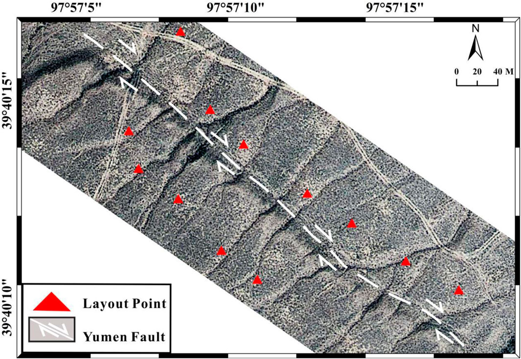
Figure 2. Google earth image of in Xigou Ore.

3.1 Point cloud collection

We used an RIEGL VZ-1000 laser scanner, a 3D laser scanning system developed by RIEGL Company (Austria) and mainly used for collecting 3D point cloud data at the dislocation of typical landforms along faults. The system consists of a laser transmitter, texture acquisition camera, and global positioning system (GPS) antenna (Figure 3); technical parameters are shown in Table 1.

Figure 3

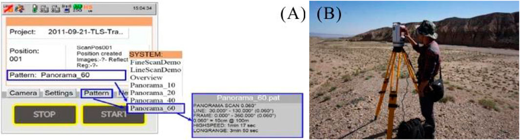
Figure 3. Ground-based LiDAR scanning setting and field work diagram. (A) Ground-based LiDAR scanning setting. (B) Field work diagram.

Table 1

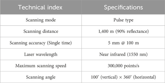
Table 1. Technical specifications of the RIEGL VZ-1000.

The ground-based LiDAR scanning survey was mainly divided into acquisition and processing procedures (Figure 4). Data acquisition where the reasonable development of the scanning scheme and site layout is according to the actual field terrain is paramount. Before data collection, the scanning parameters of each station should be set according to the actual working requirements (Figure 3A), such as scanning distance, camera exposure, device storage, and GPS check. During data acquisition, the tripod should be as stable as possible to reduce jitter, and attention should be given to the heat dissipation and power supply of the instrument. The second part is point-cloud processing analysis. The first stage of this part is point cloud pretreatment—mainly filtering, registration, and density—and the second stage is point cloud application analysis, which mainly includes interpolation filling, 3D modeling, application research, and analysis.

Figure 4

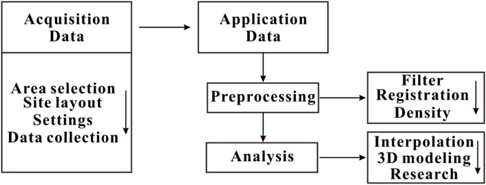
Figure 4. Flow chart of ground-based LiDAR working.

3.2 Point cloud processing

3.2.1 Point cloud filter

LiDAR technology can remove surface vegetation information via the filtering method. In the preprocessing stage, point cloud filters non-terrain target information, such as houses, trees, and telephone poles. Better topographic and surface information are obtained through the filtering processing to reconstruct model. Noise and errors are inevitable when ground-based LiDAR collects point cloud data, and this information cannot be used directly (Zheng, 2005). Thus, the filtering process improves the accuracy of subsequent data processing and modeling.

This study employed neighborhood statistical analysis based on each point to determine irregular shape and high-density features of topographic cloud data. This method calculates the average distance of its neighbor domain to obtain the Gaussian distribution using the mean and standard deviation (Jiao, 2015). Points with average distances exceeding the standard range are regarded as noise points and are thus removed. Considering the local point cloud data of the Yumen Fault as an example, 2,696,180 laser points were input. After numerous tests, when the adjacent points participating in the statistics were set as 50 and the noise point threshold was set as 1, the number of point cloud result points was 2,552,017 and noise points was 144,163. As shown in Figure 5, the point cloud adequately preserves the terrain information and allows for the effective elimination of the noise points, indicating that the parameter settings are reasonable.

Figure 5

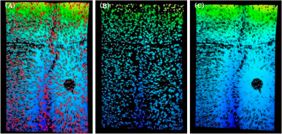
Figure 5. Removal of noise point cloud data. (A) Original data; red dots represent the distribution of noise points generated by the jump boundary and the atmosphere; (B) deleted noise point cloud data; (C) ground point cloud data after noise removal.

3.2.2 Point cloud registration

Point cloud registration aims to comprehensively obtain topographic and geomorphic surface information on the study area, translating and rotating the point cloud information measured by multiple angles and sites to achieve coordinate unification and comprehensively obtain data. During data collection, the perspective range of each site should be determined to ensure sufficient overlapping areas between adjacent sites for point cloud registration between sites. As shown in Figure 6, the same scanner scans object P in the research area at different positions A and B. Position A records the 3D coordinate information O1 (X₁, Y₁, Z₁) at P, while position B records the 3D coordinate information O2 (X₂, Y₂, Z₂) at P. Scanning information is obtained at two different positions. Point cloud data obtained in these different coordinate systems is converted to the same coordinate system in the subsequent data registration.

Figure 6

Figure 6. Scanning of the same point by different sites.

Due to the complex topography and abundant vegetation on both sides of the Fault scarp in the study area, multiple scanning stations were implemented in the collection process to ensure higher data accuracy and reduce data vulnerabilities. In data processing, this study improved computational efficiency by using the ICP algorithm based on grid splicing proposed by Jiao (2015). Taking Scan01 and Scan02, the search distance between point clouds is firstly set as 5 m, duration as 6 s, with the residual result of 0.0562; its residual distribution histogram is shown in Figure 7A. Secondly, after several iterations of registration, the final setting distance was 0.5 m, the duration 1 s, and the residual 0.0188; its residual distribution histogram is shown in Figure 7B, and the time, error, and residual of the first and last iteration registration are shown in Table 2. When the standard deviation is below 0.005 m, it is regarded as a complete match, and the registration accuracy of adjacent stations is the highest. The final multi-station sub-point cloud data registration is shown in Figure 8.

Figure 7

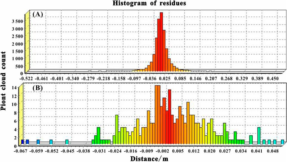
Figure 7. Histogram of residual distribution for multiple iteration registration. (A) The first histogram of residual distribution. (B) The final hisrogram of residual disrtribution.

Table 2

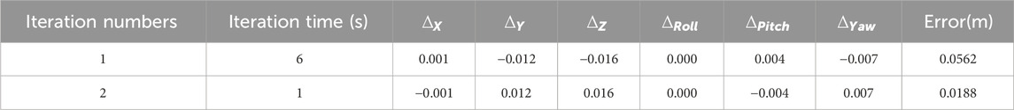
Table 2. Iteration registration errors and residuals.

Figure 8

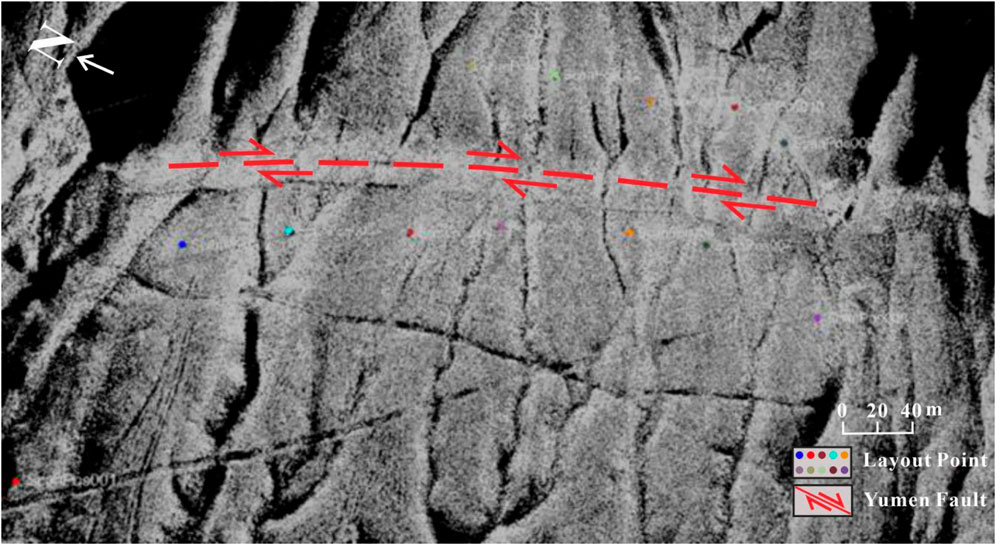
Figure 8. Effect diagram of point cloud registration.

3.2.3 Point cloud density

Ground-based LiDAR scans with small spacing result in more point clouds to capture detailed elevation data of topography surfaces. Furthermore, the high elevation capacity information in point cloud data increases the computational load during DEM creation (Song and Feng, 2008; Buckley et al., 2008). To improve DEM accuracy, point cloud data can be compressed, simplified, and made redundant using appropriate methods. This reduces the data needed to approximate the original terrain model, shortening the reconstruction time and reducing resource waste.

In this study, point cloud data were successively compressed according to the compression grade (100%, 75%, 50%, 20%, and 10%) raw data. The point cloud data set was compressed via GIS spatial statistical analysis, and the corresponding DEM generated by the interpolation of point cloud data set was compressed by each density level. Two common DEM accuracy indexes—mean error (ME) and standard deviation (SD) —were selected for evaluation (Jiao, 2015; Li et al., 2011; Hodgson et al., 2003). To compare the accuracy levels of the DEM for different density levels, the DEM elevation value of 100% point-cloud density assumed the true value Z, and the DEM high value of other density levels assumed the predicted value, z. The error expressed as S = Z-z. n was set as the corresponding number of elevation points, then the mean error, standard deviation, and root mean square error were calculated thus:

Mean Error (ME)

$\mathbf{\text{ME}}={\displaystyle \sum _{i=1}^n}\frac{{\epsilon }_i}{n}$

Standard Deviation (SD)

$\mathbf{\text{SD}}=\sqrt{{\displaystyle \sum _{\mathrm{i}=1}^{\mathrm{n}}}\frac{{\left({\mathrm{\epsilon }}_{\mathrm{i}}-\text{ME}\right)}^2}{\mathrm{n}}}$

—where $\epsilon$ is the error and $i$ is the number of points.

As the DEMs for all density levels were generated with the same resolution, they have a common number of grids, and their grid units correspond. Therefore, the DEM files of each density raster are first converted to point element files; the number of points is the same as the number of rasters, and the point element attribute is the elevation value of the center of its corresponding raster cell. To determine the error statistics, 10,000 points were randomly selected from the DEM of each density level. Figures 9A–E shows that the number of elevation points gradually decreases as the point cloud density level decreases and point clouds become increasingly sparse. Meanwhile, for DEM corresponding to each density, it is difficult to determine the difference in its information content by only human observation (Figures 9A–E). This necessitates statistical analysis of the relevant parameters of DEM generated by each density level (Table 3) to quantitatively and intuitively show the differences between different cloud compressed density data sets and their corresponding DEM. As the point cloud compression density decreases, the total number of point clouds at each level gradually decreases from the original 779,452 to 77,945. At the same time, with the same horizontal resolution, the number of points contained in unit grid cells also gradually decreased under the premise of the same total number of DEM grids. Within the 100%–20% range, the mean elevation and standard deviation decrease as density decreases, although the amplitude is small. To achieve efficient and rapid acquisition of topographic and geomorphic model results, the calculation cost is reduced, and to ensure modeling accuracy, the optimal point cloud compression density was determined to be 20% based on the research and analysis of the optimal point cloud density of micro-topographic DEM.

Figure 9

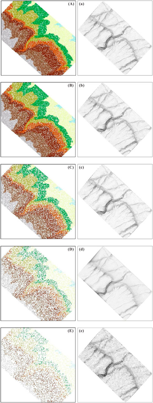
Figure 9. Point cloud data of different densities and corresponding DEM. Point cloud density: (A) 100%; (B) 75%; (C) 50%; (D) 20%; (E) 10%, corresponding to the DEM for (a–e), respectively.

Table 3

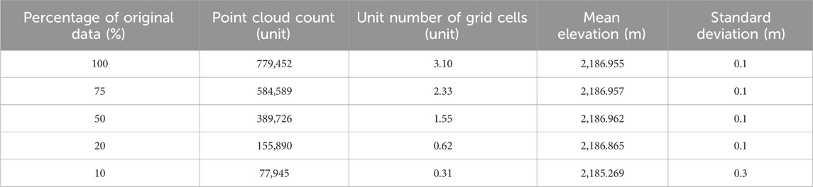
Table 3. DEM parameters generated by each density level.

4 Point cloud data analysis and application

4.1 Point cloud data interpolation modeling

In topographic and geomorphic application by ground-based LiDAR, instrument jitter, complex terrain, occluders, and other uncertain factors may cause data loss during the acquisition process (black area in Figure 8), thus affecting the integrity of terrain model establishment. A reasonable spatial interpolation algorithm can ensure the application research of point cloud data in the subsequent period. Spatial interpolation technology is fundamental to the determination of discrete points or surfaces in the form of known data. To determine the correlation function algorithm, its approximation to the real space distribution must be optimized, and the space of other function characteristic values of unknown points or partitions must be calculated according to the algorithm, as setting a continuous surface can show the surface information more intuitively.

By comparing the application of different interpolation methods of point cloud data in the topographic landform, the triangulated irregular network (TIN) can adequately fill the omissions of point cloud data and can accurately represent its elevation attribute information according to the real terrain changes (Kang et al., 2020; Yao et al., 2014). The principle of TIN is as follows. Triangle construction is carried out to form a grid range that can cover the entire region; the triangles constructed cannot intersect, and the faces of the network nodes covered by each triangle are regarded as known information. All points in the constructed triangle are limited by the surface of the triangle (Figure 10). Therefore, TIN was adopted to fill the point cloud data in this study; the results are shown in Figure 11.

Figure 10

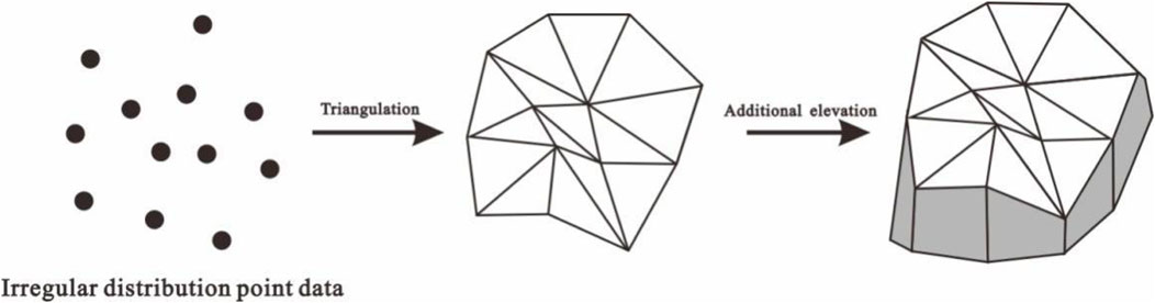
Figure 10. Interpolation diagram of the triangulation irregular network (TIN).

Figure 11

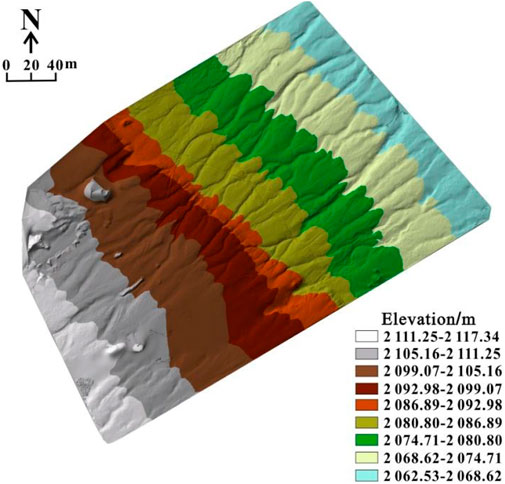
Figure 11. Interpolation effect picture of TIN.

4.2 Geomorphic fault measurement and analysis

The study area is located in the western area of Xigou Ore in the western section of the Yumen Fault, an uninhabited area of the Gobi Desert, where the multi-stage alluvial fan front is influenced by the Yumen Fault. High-resolution remote sensing enabled a satellite to identify a surface rupture zone with linear characteristics, rupturing all the alluvial fans along several gullies, except for the latest gully. A number of gullies have been broken by the fault, forming an obvious dextral curve (Figure 2).

4.2.1 Horizontal dislocation measurement and analysis

Professional software (RISCAN-PRO and ArcGIS, for example) was utilized to process point cloud data and read topographic data, resulting in high-precision topographic and geomorphic maps. High-density point cloud data were used to create a geometric high-definition 3D model of surface rupture in the Xigou Ore local regions of the Yumen Fault. We used high-density point cloud data to create a 0.1 m high-resolution DEM and a geomorphic shadow map, which were then used to build a topographic map with a contour distance of 0.5 m (Figure 12). The topographic map was utilized as the basis map to analyze the region’s structural topography and geomorphology (Figure 13). Other work was done in addition to measuring the fault geomorphic displacement.

Figure 12

Figure 12. Geomorphological map of Xigou Ore in the Yumen Fault (contour interval 0.5 m).

Figure 13

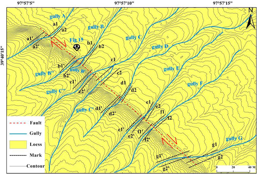
Figure 13. Geomorphical fault interpretation analysis diagram (contour interval 0.5 m).

The high-resolution remote sensing images and field investigation results showed that the surface rupture zone at the west side of Xigou Ore has obvious dextral strike–slip displacement in several gullies caused by earthquakes (Figure 13). As shown in Figure 13, the normal strike of gully B and gully C should be along gully B′ and gully C′, respectively. However, the earthquake caused obvious dextral dislocation at the fault trace, forming new gullies B″ and C″. Gullies B′ and C′ are ancient and abandoned owing to the occurrence of the earthquake, but gully C′ has been well preserved because of long-term rain erosion. Considering gully B as an example, the LaDiCaoz tool is a displacement measurement tool developed by Zielke and Arrowsmith (2012) based on Matlab and is used to measure gully displacement (Figure 14). As shown in Figure 14A, through horizontal or vertical stretching, when the mismatching value is lowest, the overlap degree of the red line and blue line is highest. Therefore, the most reasonable recovery position of the slope of the dislocation terrain was obtained. By the vertical or horizontal stretching and moving of gully B″, the dislocation topographic profile on both sides of the fault obtained the optimal recovery position. The optimal horizontal displacement of gully B″ is 8.7 m (Figure 14B). According to the geological marker in Figure 13, the distance between markers b1 and b1′ is 9.1 m, and the distance between markers b2 and b2′ is 8.3 m. The error range of this gully is approximately 0.4 m, so, the horizontal dislocation of gully B is 8.7 ± 0.4 m (Figure 14C). Therefore, the displacements of gullies A, C, D, E, F, and G are 7.4 ± 0.2 m, 15.3 ± 0.3 m, 4.8 ± 0.5 m, 5.0 ± 0.3 m, 2.3 ± 0.4 m, and 13.9 ± 0.1 m, respectively. The displacements of gullies A, B, C, and G are large and presumably caused by multiple seismic events, while the displacements of gullies D, E, and F were small and presumably caused by a single seismic event.

Figure 14

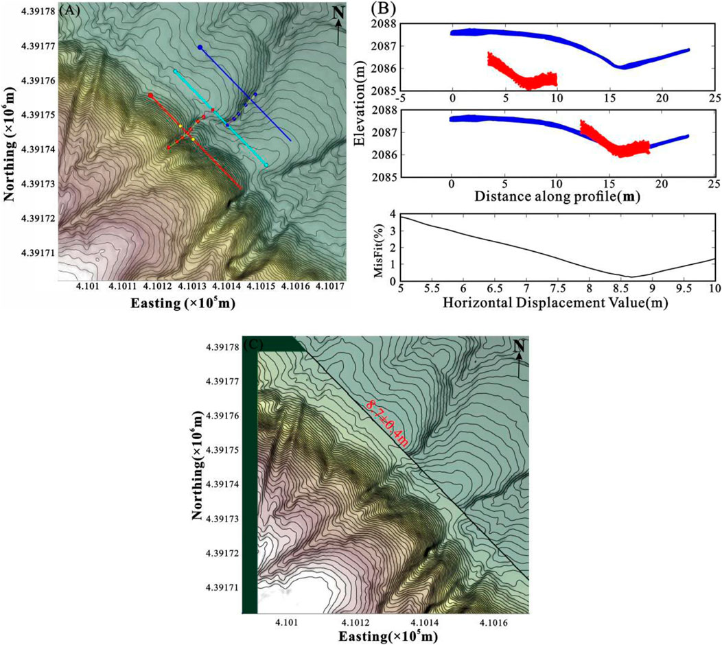
Figure 14. Measurement map of gully dislocation recovery of the Yumen Fault. (A) Mountain shadow map of gully B; light-colored line is the fault location, red and blue lines are the topographic profiles of gully B, and yellow line is the trend of gully B on both sides of the fault. (B) Original topographic profile (top), restored gully topographic profile (middle), nd displacement mismatch distribution (bottom). (C) Mountain shadow map after dislocation recovery of gully B.

4.2.2 Vertical dislocation measurement and analysis

The Yumen Fault features a thrust nappe, and many fault scarps are formed along the surface rupture zone, which can be regarded as the vertical distance of fault activity. To reflect the movement characteristics of the fault thrust nappe, this study used high-density point cloud data to generate high-precision DEM and performed topographic profile analysis with the same distance along the direction across the surface rupture. As shown in Figure 15, fault scarps are obvious, and each profile has a certain scarp height. The four scarps are 7.5 m, 8.5 m, 6.5 m, and 7.5 m high. Based on exploration and dating in this area, the surface rupture in Xigou Ore was inferred to have been formed by earthquake induction during the Holocene and to have undergone four paleoseismic events (Li et al., 2016). Therefore, the average height of the steep ridge formed in the four paleoseismic events in this area can be inferred to be approximately 6.9 ± 1.6 m, and the average height of the steep ridge caused by each seismic event approximately 1.7 ± 0.4 m.

Figure 15

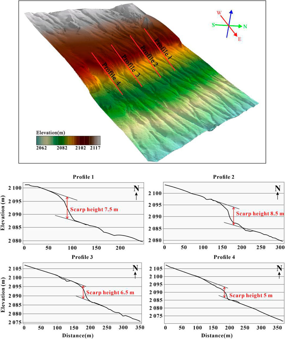
Figure 15. Vertical displacement profile of the Yumen Fault.

5 Conclusion

In this study, ground-based LiDAR measurement technology was used to collect the high-precision point cloud data of a typical fault steeper on the west side of Xigou Ore in the western section of the Yumen Fault. The high-precision point cloud data in the study area were obtained through data preprocessing such as point cloud filtering, registration, and density selection. Furthermore, 3D analysis of the fault steeper was carried out using TIN and other processing techniques. The quantitative information on fault scarps can be measured in any azimuth, and the micro-geomorphic morphology of fault scarps on the west side of Xigou Mine in the western section of the Yumen Fault can be obtained. The following are the main conclusions of this study.

(1) ICP is relatively suitable for ground-based LiDAR multi-station sub-point cloud data registration and exhibits high levels of efficiency and precision.

(2) The optimal point cloud density of microtopographic DEM was studied and analyzed, and the optimal point cloud compression density was selected as 20% to allow for quick terrain modeling with high precision.

(3) Based on point cloud data processing, a spatial resolution of 0.1 m DEM was applied to classify the geomorphic unit, identify the fault scarp and broken gully terrain information, and quantitatively study and analyze the horizontal gully dislocation and displacement distance of the fault scarp. Surface rupturing earthquakes are inferred to have occurred in the Yumen Fault during the Holocene, accompanied by typical dextral strike–slip and vertical uplift.

LiDAR data were applied in the study of the Yumen Fault, thus overcoming the limitations of general remote sensing data in the fine study of microgeomorphology, given its limited precision. Furthermore, this study enriched the quantitative analysis methods of structural geomorphology and improved the key technologies of ground-based LiDAR data processing, information recognition, and extraction oriented to the application of active structures. The high-density point cloud data collected in the western section of the Yumen Fault can provide new data supporting subsequent research on fine mapping, geometric roughness, and fault complexity. Furthermore, it creates conditions for subsequent comparison of geological and fault strain accumulation rates.

Data availability statement

The raw data supporting the conclusions of this article will be made available by the authors without undue reservation.

Author contributions

SK: conceptualization, funding acquisition, methodology, visualization, writing – original draft, writing – review and editing. QJ: conceptualization, methodology, and writing – original draft. LJ: funding acquisition, project administration, writing – review and editing. YZ: data curation, investigation, writing – review and editing. CC: data curation, investigation, writing – review and editing.

Funding

The author(s) declare that financial support was received for the research and/or publication of this article. This research was funded by the Spark Programs of Earthquake Sciences granted by the China Earthquake Administration (XH254309YA), National Natural Science Foundation of China (42474013), and the Natural Science Foundation of Shaanxi Province, China (2025JC-YBQN-463).

Conflict of interest

The authors declare that the research was conducted in the absence of any commercial or financial relationships that could be construed as a potential conflict of interest.

Generative AI statement

The author(s) declare that no Generative AI was used in the creation of this manuscript.

Publisher’s note

All claims expressed in this article are solely those of the authors and do not necessarily represent those of their affiliated organizations, or those of the publisher, the editors and the reviewers. Any product that may be evaluated in this article, or claim that may be made by its manufacturer, is not guaranteed or endorsed by the publisher.

References

Baran, R., Guest, B., and Friedrich, A. M. (2010). High-resolution spatial rupture pattern of a multiphase flower structure, Rex Hills, Nevada: new insights on scarp evolution in complex topography based on 3-D laser scanning. Geol. Soc. Am. Bull. 122 (5-6), 897–914. doi:10.1130/B26536.1

CrossRef Full Text | Google Scholar

Begg, J. G., and Mouslopoulou, V. (2010). Analysis of late Holocene faulting within an active rift using lidar, Taupo Rift, New Zealand. J. Volcanol. Geotherm. Res. 190 (1-2), 152–167. doi:10.1016/j.jvolgeores.2009.06.001

CrossRef Full Text | Google Scholar

Bello, S., Lavecchia, G., Andrenacci, C., Ercoli, M., Cirillo, D., Carboni, F., et al. (2022). Complex trans-ridge normal faults controlling large earthquakes. Sci. Rep. 12 (1), 10676. doi:10.1038/s41598-022-14406-4

PubMed Abstract | CrossRef Full Text | Google Scholar

Bello, S., Scott, C. P., Ferrarini, F., Brozzetti, F., Scott, T., Cirillo, D., et al. (2021). High-resolution surface faulting from the 1983 Idaho Lost River Fault Mw 6.9 earthquake and previous events. Sci. Data 8 (1), 68. doi:10.1038/s41597-021-00838-6

PubMed Abstract | CrossRef Full Text | Google Scholar

Bi, L. S., He, H. L., Xu, Y. R., Wei, Z. Y., and Shi, F. (2011). The extraction of knickpoint series based on the high resolution DEM data and the identification of paleoearhthquake series—a case study of the Huoshan MTS. piedmont fault. Seismol. Geol. Chin. 33 (4), 963–977. doi:10.3969/j.issn.0253-4967.2011.04.019

CrossRef Full Text | Google Scholar

Buckley, S. J., Howell, J. A., Enge, H. D., and Kurz, T. H. (2008). Terrestrial laser scanning in geology; data acquisition, processing and accuracy considerations. J. Geol. Soc. 165 (3), 625–638. doi:10.1144/0016-76492007-100

CrossRef Full Text | Google Scholar

Carter, W. E., Shrestha, R. L., and Slatton, K. C. (2007). Geodetic laser scanning. Phys. Today 60 (12), 41–47. doi:10.1063/1.2825070

CrossRef Full Text | Google Scholar

Chen, B. L., Wang, C. Y., Cui, L. L., and Liu, J. M. (2009). Developing model of thrust fault system in western part of northern Qilian Mountains margin-Hexi Corridor basin during late Quaternary. Earth Sci. Front. 15 (6), 260–277. doi:10.3321/j.issn:1005-2321.2008.06.033

CrossRef Full Text | Google Scholar

Chen, T., Zhang, P. Z., Liu, J., Li, C. Y., Ren, Z. K., and Hudnut, K. W. (2014). Quantitative study of tectonic geomorphology along Haiyuan fault based on airborne LiDAR. Chin. Sci. Bull. 59 (14), 2396–2409. doi:10.1007/s11434-014-0199-4

CrossRef Full Text | Google Scholar

Cirillo, D., Cerritelli, F., Agostini, S., Bello, S., Lavecchia, G., and Brozzetti, F. (2022). Integrating post-processing kinematic (PPK)–Structure-from-Motion (SfM) with unmanned aerial vehicle (UAV) photogrammetry and digital field mapping for structural geological analysis. ISPRS Int. J. Geo-Information. 11 (8), 437. doi:10.3390/ijgi11080437

CrossRef Full Text | Google Scholar

Crosby, C. J., Arrowsmith, J. R., and Nandigam, V. (2020). Zero to a trillion: advancing Earth surface process studies with open access to high-resolution topography. Remote Sens. Geomorphol. 23, 317–338. doi:10.1016/B978-0-444-64177-9.00011-4

CrossRef Full Text | Google Scholar

Deng, Q. D., Zhang, P. Z., Ran, Y. K., Yang, X. P., Min, W., and Chu, Q. Z. (2002). Basic characteristics of active tectonics of China. Scinece China Ser. D 32 (12), 1020–1030. doi:10.3969/j.issn.1674-7240.2002.12.007

CrossRef Full Text | Google Scholar

Haddad, D. E., Akciz, S. O., Arrowsmith, J. R., Rhodes, D. D., Oldow, J. S., Zielke, O., et al. (2012). Applications of airborne and terrestrial laser scanning to paleoseismology. Geol. Soc. Am. 8, 771–786. doi:10.1130/GES00701.1

CrossRef Full Text | Google Scholar

Harding, D. J., and Berghoff, G. S. (2000). “Fault scarp detection beneath dense vegetation cover,” in Airborne lidar mapping of the Seattle fault zone. Washington State: Bainbridge Island.

Google Scholar

He, H. L. (2011). Some problems of aerial photo interpretaion in active fault mapping. Seismol. Geol. (in Chinese) 33 (4), 938–950. doi:10.3969/j.issn.0253-4967.2011.04.017

CrossRef Full Text | Google Scholar

Hilley, G. E., and Arrowsmith, J. R. (2008). Geomorphic response to uplift along the Dragon's Back pressure ridge, Carrizo Plain, California. Geology 36 (5), 367–370. doi:10.1130/G24517A.1

CrossRef Full Text | Google Scholar

Hodgson, M. E., Jensen, J. R., Schmidt, L., Schill, S., and Davis, B. (2003). An evaluation of lidar- and ifsar-derived digital elevation models in leaf-on conditions with usgs level 1 and level 2 dems. Remote Sens Environ 84, 295–308. doi:10.1016/S0034-4257(02)00114-1

CrossRef Full Text | Google Scholar

Hudnut, K. W. (2002). High-resolution topography along surface rupture of the 16 october 1999 hector mine, California, earthquake (m_w 7.1) from airborne laser swath mapping. Bulletin of the Seismological Society of America 92 (4), 1570–1576. doi:10.1785/0120000934

CrossRef Full Text | Google Scholar

Jiang, W. L., Han, Z. J., Guo, P., Zhang, J. F., Jiao, Q. S., Kang, S., et al. (2017). Slip rate and recurrence intervals of the east Lenglongling Fault constrained by morphotectonics; tectonic implications for the northeastern Tibetan Plateau. Lithosphere 9 (3), 417–430. doi:10.1130/L597.1

CrossRef Full Text | Google Scholar

Jiang, W. L., Zhang, J. F., Shen, X. H., Jiao, Q. S., Tian, T., and Wang, X. (2018). Geometric and geomorphic features of active fault structures interpreted from high-resolution remote sensing data. Journal of Remote Sensing 22 (Sup), 192–211. doi:10.11834/jrs.20187193

CrossRef Full Text | Google Scholar

Jiao, Q. S. (2015). “The buildings earthquake damage analysis based on LiDAR”. Institute of Engineering Mechanics, China Earthquake Administration. PhD dissertation.

Google Scholar

Jiao, Q. S., Jiang, W. L., Zhang, J. F., Jiang, H. B., Luo, Y., and Wang, X. (2016a). Identification of paleoearthquakes based on geomorphological evidence and their tectonic implications for the southern part of the active Anqiu-Juxian fault, eastern China. Journal of Asian Earth Sciences 132, 1–8. doi:10.1016/j.jseaes.2016.10.012

CrossRef Full Text | Google Scholar

Jiao, Q. S., Zhang, J. F., Jiang, H. B., Su, Y. Y., and Wang, X. (2016b). Typical earthquake damage extraction and three-dimensional modeling analysis based on terrestrial laser scanning: a case study of Bailu middle school of Pengzhou City. Remote Sensing for Land and Resources 28 (1), 166–171. doi:10.6046/gtzyyg.2016.01.24

CrossRef Full Text | Google Scholar

Johnson, K., Nissen, E., Saripalli, S., Arrowsmith, J. R., Mcgarey, P., Scharer, K., et al. (2014). Rapid mapping of ultrafi ne fault zone topography with structure from motion. Geosphere 10 (5), 969–986. doi:10.1130/GES01017.1

CrossRef Full Text | Google Scholar

Kang, S., Ji, L. Y., Jiao, Q. S., and Zhang, J. F. (2020). Comparative study of point cloud data interpolation based on ground-based LiDAR. Journal of Geodesy and Geodynamics 40 (4), 400–404. doi:10.14075/j.jgg.2020.04.015

CrossRef Full Text | Google Scholar

Klinger, Y., Etchebes, M., Tapponnier, P., and Narteau, C. (2011). Characteristic slip for five great earthquakes along the Fuyun fault in China. Nature Geoscience. Nat. Geosci. 4 (6), 389–392. doi:10.1038/NGEO1158

CrossRef Full Text | Google Scholar

Li, A., Wang, X. X., Zhang, S. M., Chen, Z. D., Liu, R., Zhao, J. X., et al. (2016). The slip rate and paleoearthquakes of the Yumen fault in the Northern Qilian mountains since the late Pleistocene. Seismology and Geology 38 (4), 897–910. doi:10.3969/j.issn.0253-4967.2016.04.008

CrossRef Full Text | Google Scholar

Li, S., MacMillan, R. A., Lobb, D. A., McConkey, B. G., Moulin, A., and Fraser, W. R. (2011). Lidar dem error analyses and topographic depression identification in a hummocky landscape in the prairie region of Canada. Geomorphology (Amst) 129, 263–275. doi:10.1016/j.geomorph.2011.02.020

CrossRef Full Text | Google Scholar

Liu, J., Chen, T., Zhang, P. Z., Zhang, H. P., Zheng, W. J., Ren, Z. K., et al. (2013). Illuminating the active Haiyuan Fault, China by airborne light detection and ranging. Chin Sci Bull Chin Ver 58, 41–45. doi:10.1360/972012-1526

CrossRef Full Text | Google Scholar

Liu, Y. H., Ji, L. Y., Zhu, L. Y., Zhang, W. T., Liu, C. J., Xu, J., et al. (2024). Postseismic deformation mechanism of the 2021 Mw7.3 Maduo earthquake, northeastern Tibetan plateau, China, revealed by Sentinel-1 SAR images. Journal of Asian Earth Sciences 265, 106089. doi:10.1016/j.jseaes.2024.106089

CrossRef Full Text | Google Scholar

Min, W., Zhang, P. Z., He, W. G., Li, C. Y., Mao, F. Y., and Zhang, S. P. (2002). Research on the active faults and paleoearthquakes in the western Jiuquan basin. Seismology and Geology 24 (1), 35–44. doi:10.3969/j.issn.0253-4967.2002.01.004

CrossRef Full Text | Google Scholar

Ran, B., Li, Y. L., Zhu, L. D., Zheng, R. C., Yan, B. N., and Wang, M. F. (2013). Early tectonic evolution of the northern margin of the Tibetan Plateau: constraints from the sedimentary evidences in the Eocene-Oligocene of the Jiuxi basin. Acta Petrologica Sinica 29 (3), 1027–1038.

Google Scholar

Ren, Z. K., Chen, T., Zhang, H. P., Zheng, W. J., and Zhang, P. Z. (2014). LiDAR survey in active tectonics studies: an introduuction and overview. Acta Geologica Sinica 88 (6), 1196–1207. doi:10.19762/j.cnki.dizhixuebao.2014.06.019

CrossRef Full Text | Google Scholar

Song, H., and Feng, H. Y. (2008). A global clustering approach to point cloud simplification with a specified data reduction ratio. Computer-Aided Design 40 (3), 281–292. doi:10.1016/j.cad.2007.10.013

CrossRef Full Text | Google Scholar

Uysal, M., Toprak, A. S., and Polat, N. (2015). DEM generation with UAV Photogrammetry and accuracy analysis in Sahitler hill. Measurement 73, 539–543. doi:10.1016/j.measurement.2015.06.010

CrossRef Full Text | Google Scholar

Wang, S. Y., Ai, M., Wu, C. Y., Lei, Q. Y., Zhang, H. P., Ren, G. X., et al. (2018). Application of DEM generation technology from high resolution satellite iamge in quantitative active tectonics study: a case study of fault scarps in the southern margin of KuMiShi basin. Seismology and Geology 40 (5), 999–1017. doi:10.3969/j.issn.0253-4967.2018.05.004

CrossRef Full Text | Google Scholar

Wechsler, N., Rockwell, T. K., and Ben-Zion, Y. (2009). Application of high resolution DEM data to detect rock damage from geomorphic signals along the central San Jacinto Fault. Geomorphology 113 (1-2), 82–96. doi:10.1016/j.geomorph.2009.06.007

CrossRef Full Text | Google Scholar

Westoby, M. J., Brasington, J., Glasser, N. F., Hambrey, M. J., and Reynolds, J. M. (2012). Structure-from-Motion’ photogrammetry: a low-cost, effective tool for geoscience applications. Geomorphology 179, 300–314. doi:10.1016/j.geomorph.2012.08.021

CrossRef Full Text | Google Scholar

Xiang, H. F., and Guo, S. M. (1990). Preliminary study on active faults in Yumen-Jiayuguan area of Hexi Corridor. Beijing: Seismological Press, 139–145.

Google Scholar

Xu, J., Liu-Zeng, J., Yuan, Z. D., Yao, W. Q., Zhang, J. Y., Ji, L. Y., et al. (2022). Airborne LiDAR-based mapping of surface ruptures and coseismic slip of the 1955 zheduotang earthquake on the xianshuihe fault, east tibet. Bulletin of the Seismological Society of America 112 (6), 3102–3120. doi:10.1785/0120220012

CrossRef Full Text | Google Scholar

Yao, Y. L., Jiang, S. P., and Wang, H. P. (2014). Comparative study of point cloud data interpolation based on ground-based LiDAR. Journal of Geomatices 39 (1), 50–53. doi:10.14188/j.2095-6045.2014.01.015

CrossRef Full Text | Google Scholar

Zheng, D. H. (2005). Theory and method of 3D laser scanning data processing. Tongji University.

Google Scholar

Zhou, L., Kaneda, H., Mukoyama, S., Asada, N., and Chiba, T. (2013). Detection of subtle tectonic–geomorphic features in densely forested mountains by very high-resolution airborne LiDAR survey. Geomorphology 182, 104–115. doi:10.1016/j.geomorph.2012.11.001

CrossRef Full Text | Google Scholar

Zielke, O., Arrowsmith, J. R., Ludwig, L. G., and Akçiz, S. O. (2010). Slip in the 1857 and earlier large earthquakes along the carrizo plain, san Andreas fault. Science 329 (5990), 390. doi:10.1126/science.329.5990.390

CrossRef Full Text | Google Scholar

Zielke, O., and Arrowsmith, R. (2012). LaDiCaoz and lidar imager — MATLAB GUIs for lidar data handling and lateral displacement measurement. Geosphere 8 (1), 206–221. doi:10.1130/GES00686.1

CrossRef Full Text | Google Scholar

Zielke, O., Klinger, Y., and Arrowsmith, J. R. (2015). Fault slip and earthquake recurrence along strike-slip faults—contributions of high-resolution geomorphic data. Tectonophysics 638, 43–62. doi:10.1016/j.tecto.2014.11.004

CrossRef Full Text | Google Scholar