Assessing SWOT interferometric SAR altimetry for inland water monitoring: insights from Lake Léman

Monitoring water levels is crucial for managing water resources and addressing climate change challenges. The new Surface Water and Ocean Topography (SWOT) mission provides unprecedented spatial and temporal resolution estimates of water surface elevations (WSEs) globally. This study evaluates the accuracy of SWOT WSE estimates over Lake Léman, Switzerland. We evaluated the SWOT L2-HR-Raster product from the calibration and nominal phases using in situ measurements of water levels and compared its performance with other missions, including Sentinel-3A (S3A), Sentinel-3B (S3B), Sentinel-6 (S6), and Global Ecosystem Dynamics Investigation (GEDI) altimetry. From over 141 acquisitions, SWOT achieved a root mean squared error (RMSE) ranging from 13 cm to 21 cm compared to in situ water levels, depending on the measurement quality reported in the product. Data flagged as good quality had an RMSE of 19 cm and a correlation coefficient (R) of 0.8, although these represented only 42% of the total measurements. When considering WSE estimates of all quality levels and applying a median outlier filter, the RMSE reaches 21 cm, with a correlation coefficient of 0.79, while retaining approximately 83% of the dataset. A consistent bias of −10 cm was observed across the time-series. An analysis of SWOT accuracy relative to instrumental parameters revealed that nadir and near-nadir acquisitions (viewing angle near 0°) exhibited very high uncertainty, with mean absolute differences from in situ water levels potentially exceeding 5 m. To explore the sources of errors in SWOT WSE, a random forest analysis showed that atmospheric perturbations had the most significant impact on the SWOT WSE estimation accuracy. These perturbations were linked to dry tropospheric delays affecting interferometric height measurements and atmospheric effects on the Ka-band sigma0 values. Compared to other missions, SWOT demonstrated slightly better accuracy than S3A, S3B, and S6, with an RMSE of 11 cm on a daily scale, compared to 13 cm, 18 cm, and 20 cm for these three Sentinel missions, respectively. All radar-based missions (S3A, S3B, S6, and SWOT) exhibited correlation coefficients exceeding 0.95 with in situ water levels. In contrast, GEDI LiDAR data showed the highest RMSE (46 cm), a bias of 27 cm, and a correlation coefficient of 0.45.

1 Introduction

Inland water bodies, including rivers, lakes, reservoirs, and wetlands, are crucial components of the Earth’s hydrological and ecological systems and serve as a life-sustaining resource not only for humans by providing fresh drinking water and irrigation but also for wildlife and ecosystems (Baron et al., 2002; Dudgeon et al., 2006). Impacted by both human activities and climate change, inland water bodies are subject to extreme events such as droughts and floods (Alderman et al., 2012; Dudgeon et al., 2006; Merz et al., 2021; Reid et al., 2019; Søndergaard and Jeppesen, 2007). Thus, accurate and consistent monitoring of inland water levels is essential for understanding hydrological dynamics, managing water resources, and addressing the challenges and impacts of climate change (Kreibich et al., 2022; Loizou and Koutroulis, 2016). The most reliable method for monitoring water levels and, consequently, water volumes involves operational networks (gauges) that track changes by recording surface water elevations over time. Due to high installation and maintenance costs, the number of these stations has declined, resulting in most lakes remaining ungauged, especially those that are difficult to access (Shiklomanov et al., 2002).

As a complement to these water level measuring networks, remote sensing technologies have become an essential source of information for monitoring inland water body levels at large scales (Cretaux et al., 2023; Papa and Frappart, 2021). Particularly, active remote sensing technologies, such as radar or light detection and ranging (LiDAR), have shown high accuracy in monitoring water surface elevations over the last four decades, with more than 20 different satellite missions (Biancamaria et al., 2017; Bogning et al., 2018; Fayad et al., 2020; Nielsen et al., 2017). Currently, seven radar altimetry missions are operational (namely, SARAL, Jason-2, CryoSat-2, HY-2A, Sentinel-3, Jason-3, and Jason-CS/Sentinel 6) along with two LiDAR missions, namely, Advanced Topographic Laser Altimeter System (ATLAS) onboard the second-generation Ice, Cloud, and Land Elevation Satellite (ICESat-2) and the Global Ecosystem Dynamics Investigation (GEDI) onboard the International Space Station (ISS).

Radar altimetry for water level estimation is obtained by deriving the radar range, which is the distance between the satellite and the surface, using dedicated algorithms known as re-trackers (Cheney, 2001). The major limitation of radar altimetry is the limited coverage of the radar ground tracks for most of the missions. Currently, most of the current radar altimetry missions are only able to monitor a small portion of the Earth’s surface, principally because this technique collects elevation measurements of the Earth’s surface at the nadir direction (Cretaux et al., 2023). CryoSat-2, in contrast, had better coverage but very low temporal resolution, with a 369-day repeat orbit at the equator. Until recently, only radar altimetry missions were capable of providing continuous, temporal, and accurate monitoring of water levels (lakes and rivers) despite their spatial and/or temporal limitations (Birkett, 1998; 1995; Cretaux et al., 2023). Since the early 1990s, preliminary studies have reported that satellite radar altimeters have the potential to monitor height variations over inland waters using the NASA Radar Altimeter (NRA) with high accuracy, reaching 11 cm, yet this capability has been limited to only very large lakes and rivers with widths greater than 1 km. As reported by Maillard et al. (2015), the accuracy of lake water levels retrieved by satellite radar altimeters could be affected by the lake size, surrounding topography, and geographic locations. Detection limitations over small lakes and rivers were later resolved using higher-frequency radar signals and re-tracking algorithms such as the Ocean Correction and Oceanographic (OCOG) and Sea Ice re-trackers, thus obtaining good water level estimation accuracy on small lakes and rivers (Baup et al., 2014; Sulistioadi et al., 2015).

Regarding radar technology used, most of the radar altimeters operate in the conventional low-resolution mode (LRM), except for Sentinel-3 and CryoSat-2, which operate in the synthetic aperture radar (SAR) mode. Due to the adoption of the new SAR altimetry technology, Sentinel-3 showed the highest accuracy in water level retrieval in an evaluation of historical and operational satellite radar altimetry missions for lake water levels performed by Shu et al. (2021). This SAR altimetry technology improved the retrieval of elevation information over more variable surfaces with different object sizes (lakes and rivers sizes) by decreasing the along-track footprint size from several kilometers to approximately 300 m. Xu et al. (2024) also validated the use of Sentinel-3 level-2 land product for monitoring monthly water levels over eight lakes in China. Their comparison with in situ water levels showed that most lakes exhibited a correlation coefficient (R) above 0.9 and RMSE below 0.5 m. They presented that Sentinel-3 data also showed consistent seasonal trends over the multi-year study period. Kittel et al. (2021) evaluated the possibility of extracting river surface elevation at the catchment level from Sentinel-3A and Sentinel-3B radar altimetry using level-1b and level-2 data. At six in situ stations on the Zambezi River in Africa, the RMSE of the S3 products was less than 32 cm. Nilsson and Nielsen (2024) validated the Sentinel-6 Michael Freilich (MF) (S6MF) low- and high-resolution lake water levels with data from 124 gauges in 85 lakes from the United States, Canada, Sweden, and Australia. The unbiased RMSE (ubRMSE) for S6MF varied between 6.4 cm and 31.3 cm for all data, with the best ubRMSE achieved when using the high-resolution mode and the OCOG re-tracker.

Since radar altimetry has been generally limited by spatial coverage, temporal revisit, and water body sizes, LiDAR altimetry appeared as complementary to radar altimetry where studies have presented a high potential of LiDAR data in estimating water levels (Fayad et al., 2020; Zhang et al., 2019). Contrary to radar altimetry, LiDAR missions such as the ICESat-2 and GEDI provide measurements over larger parts (higher spatial coverage) of the Earth through their small footprints (higher spatial resolution). ICESat-2 and GEDI showed acceptable accuracy in estimating water levels (Fayad et al., 2022a) despite both being launched for different objectives, with ICESat-2 designed to monitor elevation changes in Greenland and Antarctica and GEDI intended to derive forest vertical structures. Zhang et al. (2019) assessed both ICESat-1 and ICESat-2 altimetry over Qinghai Lake and reported an excellent agreement with in situ measurements with an RMSE reaching 10 cm for data collected between 2003 and 2018. Ryan et al. (2020) also assessed the first-year data of ICESat-2 altimetry over 3,712 global reservoirs and found that ICESat-2 well-retrieved water level changes with an accuracy reaching ±14 cm. Yuan et al. (2020) also evaluated ICESat-2 altimetry over all lakes in China (with a surface area >10 km²) and concluded that ICESat-2 greatly improved the altimetric capabilities with a relative altimetric error of 6 cm. GEDI became operational in 2019, and a study by Fayad et al. (2020) was among the first to assess GEDI accuracy for inland water bodies. Over the eight largest lakes in Switzerland, a small subset of GEDI data (available until 2020) showed that GEDI elevation estimates exhibit overall good agreement with in situ water levels, with a mean elevation bias of 0.61 cm and a standard deviation (std) of 22.3 cm. Over the five North American Great Lakes, Fayad et al. (2022a) analyzed the precision of the GEDI elevations, which showed an average difference from in situ elevations (bias) varying between 0.26 and 0.35 m and an RMSE ranging between 0.54 and 0.68 m. Over the Great Lakes and lower Mississippi River, Xiang et al. (2021) showed that the RMSE of GEDI elevations compared to 22 gauging stations reached 0.28 m with a bias of −0.10 m ± 0.23 m. However, they showed that GEDI had the lowest accuracy against its competitor laser altimetric missions, such as ICESat-1 and ICESat-2.

In December 2022, a collaboration between the French National Center of Spatial Studies (CNES) and the National Aeronautics and Space Administration (NASA) launched the first space mission dedicated to continental hydrology, including the monitoring of rivers and lakes: the Surface Water Ocean Topography (SWOT) (Fu et al., 2024). To overcome previous limitations of spatial coverage and water body sizes, SWOT is expected to provide new perspectives for hydrology and hydrodynamics at unprecedented spatial and temporal resolution as it permits obtaining an almost complete monitoring of inland water bodies at a spatial resolution of 100 m and a repeat cycle of 21 days (Biancamaria et al., 2016). The SWOT mission provides global water surface elevation (WSE) and inundation extent derived from high rate (HR) measurements from the Ka-band Radar Interferometer (KaRIn) (Fjortoft et al., 2014). The novelty of the SWOT mission is that it simultaneously uses two SAR antennas operating at Ka-band and separated by 10 m to perform interferometric SAR (InSAR) measurements, thus obtaining 2D WSE maps.

The main objective of this study is to evaluate SWOT WSE estimations over Lake Léman, the greatest lake in Europe, using the Level-2 High-Rate Raster (L2-HR-Raster) product, which provides WSE in geographically fixed scenes at a spatial resolution of 100 m. SWOT WSE is compared to in situ gauge stations over the period between 31 March 2023 and 01 September 2024, including data from both the calibration/validation phase (daily orbits) and the nominal phase (21 days orbit). In addition, the paper investigates the main parameters explaining the errors affecting the SWOT WSE estimates. This is achieved through an explanatory random forest (RF) analysis that integrates instrumental and geophysical information provided by the L2-HR-Raster product. Finally, the paper provides a comparison of SWOT WSE to competitor radar altimetric missions (Sentinel-3A, Sentinel-3B, and Sentinel-6) and LiDAR missions (GEDI). The main findings provide end-users with a full understanding of the L2-HR-Raster data quality and, thus, precautions for operational use.

2 Materials

2.1 Study area

2.1.1 Lake Léman

This study was carried out at Lake Geneva, also known as Lake Léman (Figure 1a), the largest lake in Central Europe in terms of both surface area and volume. Situated on the northern side of the Alps, Lake Léman is shared between Switzerland, which accounts for 60% of its surface, and France, which covers the remaining 40%. The lake has a total area of 580 km², with an average depth of 80 m and a maximum depth of 310 m, found in the expansive section between Évian-les-Bains and Lausanne, located on the French side.

Figure 1

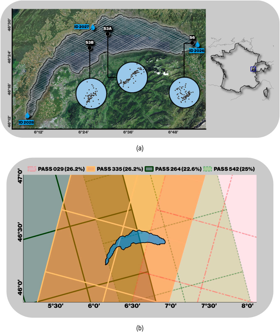
Figure 1. (a) Location of Lake Léman with the three in situ gauge stations. White points on the lake’s surface represent the distribution of the GEDI shots. Black points indicate the location of Sentinel footprints. (b) SWOT passing orbits (pass) crossing Lake Léman. The number in parentheses represents the percentage of acquisition dates for each orbit relative to the total number of acquisitions used in this study.

2.1.2 In situ water levels

The Hydrology Department of the Federal Office for the Environment (FOEN) provides surface water levels through a network of 260 gauging stations in Switzerland (www.hydrodaten.admin.ch; accessed on 03 February 2025). Water levels of Lake Léman were obtained from three gauge stations, namely, the Chillon (ID 2026), the St-Prex (ID 2027), and the Sécheron (ID 2028) stations (shown in Figure 1), and they were used to validate the SWOT, Sentinel, and GEDI altimetry-based water level estimates. Over the studied period between 2016 and 2024, the difference between the water levels measured at the three stations was negligible. As shown in Table 1, the mean difference in water levels between any two stations did not exceed 2.2 cm, with a standard deviation ranging between 1.1 and 1.5 cm over the whole period. For this reason, on each date, the average water level from the three stations was considered representative of the WSE at that given date.

Table 1

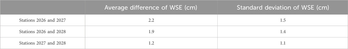
Table 1. Differences in the water level between the three in situ gauge stations in Léman Lake.

2.2 Remote-sensing water level estimation

This section provides a detailed description of the remotely sensed water level data used in the study. Table 2 summarizes the primary characteristics of all products employed, including the SAR (SWOT, Sentinel-3, and Sentinel-6) and LiDAR (GEDI) data. These datasets are presented in the following subsections.

Table 2

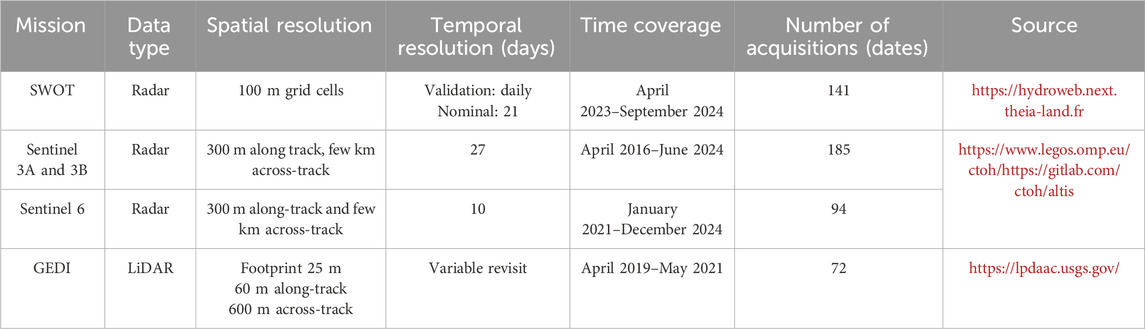
Table 2. Summary of the main remote-sensing water level estimation products used in this study.

2.2.1 SWOT mission and product

The SWOT mission, jointly developed by the CNES and NASA, with contributions from the Canadian Space Agency (CSA) and the United Kingdom Space Agency (UKSA), was launched on 15 December 2022. The main objective of this mission is to measure both ocean and continental surface water levels (rivers and lakes), making it the first space mission dedicated to continental hydrology (Fu et al., 2024). The SWOT mission’s operation began with a 3-month phase for engineering checking (January–March 2023), followed by a calibration/validation phase of 3 months on a daily sampling orbit (April–June 2023), and then the scientific phase on an orbit with a 21-day repeat period since July 2023. The SWOT mission mainly measures WSE and extent, which are used to derive river longitudinal profiles and slopes, lake water levels, and the shapes and extents of rivers and lakes between 78°N and 78°S. The SWOT mission has a cycle of 21 days, with a temporal revisit depending on the location on Earth (Biancamaria et al., 2016; Fjortoft et al., 2014). The satellite payload is composed of several instruments, including the KaRIn and Poséidon-3C nadir altimeter operating at Ku- and C-bands. The KaRIn instrument is composed of two synthetic aperture radars (SARs) operating at Ka-band. The novelty of this mission is the simultaneous use of the two SAR antennas separated by 10 m to perform interferometry (InSAR) measurements, thus obtaining 2D WSE maps (Fjortoft et al., 2014). Images have a spatial resolution of 6 m along the satellite direction and from 10 to 60 m in the range direction in the radar projection. For the geolocated projection, the final pixel size is 22 m in the azimuth direction.

A total of seven products for continental hydrology are freely available from the CNES (https://hydroweb.next.theia-land.fr; last access on 16/01/2025) and NASA data catalogs (https://search.earthdata.nasa.gov/; last access on 16/01/2025):

• L2_HR_PIXC: water mask pixel cloud

• L2_HR_PIXCVec: water mask pixel cloud auxiliary data

• L2_HR_Raster: raster NetCDF at 100 m or 250 m spatial resolution

• L2_HR_RiverSP: river single pass shapefile (reaches and nodes)

• L2_HR_RiverAvg: river cycle-averaged pass shapefile (reaches and nodes)

• L2_HR_LakeSP: lake vector single pass shapefile

• L2_HR_LakeAvg: lake vector cycle-averaged shapefile

The product used in this study is the “L2_HR_Raster” (latest version C), which contains rasterized water-surface elevations and inundation extent data from the HR data stream of the KaRIn instrument. This product is generated using L2_HR_PIXC and L2_PIXCVec products. Finally, the spatial resolution of the product is 100 m.

Over Lake Léman, a total of 141 acquisitions (each in the form of gridded points of 100 m spacing) have been used from 31 March 2023 to 01 September 2024, with 89 acquisitions during the calibration/validation phase (daily orbit, between 31 March and 31 July 2023) and 52 acquisitions during the nominal phase (21-day orbit, since August 2023). The passing orbits of the used SWOT acquisitions are presented in Figure 1b, including the percentage of acquisitions for each orbit with respect to the total number of acquisitions. In Figure 1b, each passing orbit shows two squares (footprints), where each corresponds to an observation to the left and right of the nadir. In this product, different parameters are available, and the main ones are summarized in Table 3. Other variables are described in the SWOT product description (SWOT, 2024).

Table 3

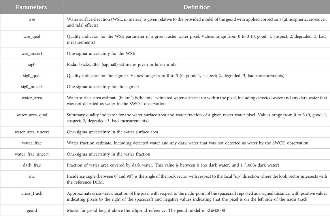
Table 3. Main SWOT parameters available in the « L2_HR_Raster » product, version C.

2.2.2 Sentinel-3 and Sentinel-6 SAR altimetry missions

Radar altimetry missions are commonly used for monitoring the elevation of inland surface water (Abdalla et al., 2021; Cretaux et al., 2023). Among them, the more recent ones operating in SAR mode are the altimetry missions developed by the European Space Agency (ESA) in the framework of the Copernicus program of the European Union (EU), including the Sentinel-3A (S3A), Sentinel-3B (S3B), and also as a continuity of the NASA-CNES Topex/Poseidon and Jason missions for Sentinel-6 Michael Freilich (S6) (Bogning et al., 2018; Normandin et al., 2018). These products use an a priori elevation [open-loop or digital elevation model (DEM)] to reduce tracking loss, which is likely to occur in mountainous areas (Biancamaria et al., 2017), and provide more accurate estimates of water surface elevation than those operating in the LRM. More details about these missions can be found in Frappart et al. (2021). Over lakes, the Sentinel missions were found to have an RMSE against in situ measurements that was lower than that of LRM missions and generally below 0.10 m (Shu et al., 2021). In over 10 Swiss lakes, including Lake Léman, comparisons made against in situ data exhibited a stable bias (−0.17 ± 0.04) m, low RMSE (<0.1 m), and generally high correlation coefficient (R) (greater than 0.85) (Frappart et al., 2021).

Time-series of water levels were derived from one Sentinel-3A (0358), one Sentinel-3B (0741), and one Sentinel-6 (044) ground track crossing Lake Léman using Altimetry Time Series (AlTiS) software (Frappart et al., 2021). This software program permits users to visualize and process the altimetry data contained in the geophysical data records (GDRs) made available by the space agencies (i.e., orbit, range, corrections to be applied to the range, and backscattering and peakiness at Ku- and C-bands). It also derives the altimeter height from the GDR data with all the necessary corrections to be applied over land. A graphical user interface helps the user in selecting the valid data to be used to obtain the time-series of water levels. This software application is commonly used to derive surface water levels over lakes and reservoirs (Aminjafari et al., 2024; de Fleury et al., 2023; Fuentes-Aguilera et al., 2024; Oularé et al., 2022; Pham-Duc et al., 2022). In this study, this software program was used to generate along-track profiles and time-series of water levels on the five Sentinel ground tracks. The geographical location of the water surface levels time-series of S3A, S3B, and S6 are shown in Figure 1.

2.2.3 GEDI data

In this study, we also compare the precision of water surface elevation provided by SWOT to elevations obtained by NASA’s recent GEDI LiDAR sensor, a full-waveform LiDAR instrument installed aboard the ISS. It is equipped with three 1,064 nm lasers, allowing it to obtain eight tracks of data represented on the ground by a series of 25-m-wide footprints spaced 60 m along the track and 600 m across the tracks (Dubayah et al., 2020). The echoed waveforms are digitized to a maximum of 1,246 bins with a vertical resolution of 1 ns (15 cm).

NASA’s Land Processes Distributed Active Archive Center (LP DAAC) processes and publishes GEDI data products of levels 1 and 2, which include the geolocated raw waveforms (L1B), footprint-level elevation and canopy height metrics (L2A), and the footprint-level canopy cover and vertical profile metrics (L2B). Two GEDI data products were used in this study, namely, level 1B (L1B) and level 2A (L2A). The GEDI L2A comprises metrics obtained with six distinct algorithms, each utilizing various thresholds and smoothing parameters on the received waveforms. From the release version V2 of the L1B data product (Dubayah et al., 2021b) and L2A data product (Dubayah et al., 2021a), we extracted the following variables derived from the processing algorithm a1, which demonstrated the best overall performance over water bodies (Fayad et al., 2022b).

• Latitude, longitude, acquisition time, and elevation of the lowest mode (i.e., surface return)

• Latitude, longitude, and elevation of the instrument

• Number of detected modes (num_detectedmodes)

• Width of the Gaussian fit to the received waveform “rx_gwidth” (hereafter referred to as gwidth)

• Amplitude of the smoothed waveform’s lowest detected mode “zcross_amp”

• Amplitude of each detected mode within the waveform “rx_modeamps”

• Mean and standard deviation of the background noise (mean and std dev)

Next, the viewing angle (VA in degrees) and the signal-to-noise ratio (SNR in decibels) were calculated for each GEDI shot (Fayad et al., 2022b; Nie et al., 2014). To calculate the SNR, the maximum amplitude within an acquired waveform, defined as the maximum of up to 19 possible values of rx_modeamps, and the mean and standard deviation of the noise are used. The distance between the location of a GEDI shot and the location of the GEDI instrument projected at the nadir onto the WGS84 reference ellipsoid and the altitude of the GEDI instrument over the referenced ellipsoid at the acquisition time of shot are used to calculate the viewing angle. VA and SNR were further used to filter unreliable GEDI shots.

The GEDI dataset comprises 72 acquisition dates, spanning from April 2019 to March 2023. Not all GEDI shots are usable since LiDAR returns can be strongly degraded due to the presence of clouds, water, and aerosols. Therefore, several filters were used to remove non-viable shots, which are later explained in the methods section (3.2 Filters for GEDI). The distribution of the GEDI shots over Lake Léman is shown in Figure 1.

3 Methods

3.1 Transformation of elevations

SWOT, Sentinel-3A, B, and 6, and GEDI elevations refer to different geodetic reference systems depending on the used geoid model. SWOT and Sentinel elevations are referenced to geoidal heights relative to the official Earth Gravitational Model EGM2008 (Pavlis et al., 2012) of the world geodetic system (WGS84), whereas GEDI elevations are referenced to ellipsoidal heights relative to the WGS84 ellipsoid. On the other hand, gauge stations of Lake Léman are measured based on the local Swiss height system referring to the CHGeo2004 Geoid model. To maintain elevation data consistency, which allows for comparing elevation estimates between different sources, it is important to first transform elevations from the different missions (SWOT, Sentinel, and GEDI) into a unified geodetic reference system. In this study, we chose to transform all elevations from SWOT, Sentinel, and GEDI to the same geoidal reference as the in situ gauges, specifically the local Swiss height reference (CHGeo2004). Figure 2 illustrates the conversion from ellipsoidal heights to geoidal heights for any reference geoidal model by accounting for the geoid–ellipsoid difference (N) where geoidal heights are given as follows:

$\mathrm{H}=\mathrm{h}-\mathrm{N},(1)$

where “N” represents the geoid undulation, “h” is the ellipsoidal height (measured perpendicular to the ellipsoid), and “H” is the orthometric height (measured from the geoid to the point of interest).

Figure 2

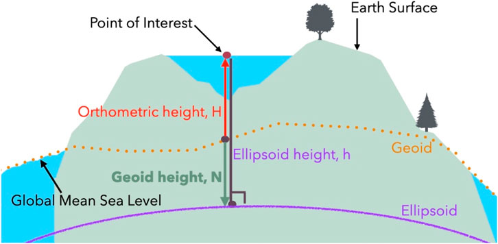
Figure 2. Illustration of the conversion from ellipsoidal heights (h) to orthometric geoidal heights (H).

SWOT and Sentinel-3A, B, and 6 data are already orthometric geoidal heights (not ellipsoidal) but refer to different geoidal references than the gauge stations (EGM2008 and CHGeo2004, respectively). Thus, the conversion of SWOT and Sentinel altimetry to Swiss geoidal based altimetry (CHGeo2004) requires an intermediate step where the WSE of these data are first reconverted to ellipsoidal heights referring to the WGS84 ellipsoid by adding back the geoidal undulation of EGM2008. Second, the WSE ellipsoidal heights are then converted to the CHGeo2004 reference by subtracting the geoidal undulation of the CHGeo2004 geoidal reference, as shown in Equation 1. The final equation for the conversion of SWOT and Sentinel WSE to the CHGeo2004 reference is provided as in Equation 2:

$\text{WS}{\mathrm{E}}_{\text{SWOT}|\text{Sentinel}}\left(\text{CHGeo}2004\right)=\text{WS}{\mathrm{E}}_{\text{SWOT}|\text{Sentinel}}\left(\text{EGM}2008\right)+{\mathrm{N}}_{\text{EGM}2008}-{\mathrm{N}}_{\text{CHGeo}2004},(2)$

Where $\text{WS}{\mathrm{E}}_{\text{SWOT}|\text{Sentinel}}\left(\text{EGM}2008\right)$ is the elevation provided by either SWOT or Sentinel, ${\mathrm{N}}_{\text{EGM}2008}$ denotes the geoid undulation for the EGM2008 system, representing the difference between the EGM2008 geoid and the WGS84 ellipsoid, and ${\mathrm{N}}_{\text{CHGEO}2004}$ represents the geoid undulation (N) for the CHGeo2004 Swiss system.

${\mathrm{N}}_{\text{EGM}2008}$ is directly provided in the SWOT products for each pixel (grid point elevation data), while for S3A, S3B, and S6, it was computed using Delaunay linear interpolation based on the global EGM2008 geoid model at 1′ resolution. The model can be accessed at the EGM2008 geoid model (https://3df-eu.fra1.digitaloceanspaces.com/geoids/EGM2008 - 1'.zip).

GEDI data are ellipsoidal heights; thus, the conversion of GEDI’s elevations to Swiss geoidal elevations directly follows Equation 1, with the N value being the geoid undulation derived from the CHGeo2004 model. GEDI geoidal elevations are thus calculated for the reference CHGeo2004 as in Equation 3:

$\text{WS}{\mathrm{E}}_{\text{GEDI}}\left(\text{CHGeo}2004\right)=\text{WS}{\mathrm{E}}_{\text{gedi}}\left(\text{Ellipsoid\hspace{0.17em}WGS}84\right)-{\mathrm{N}}_{\text{CHGeo}2004},(3)$

Where $\text{WS}{\mathrm{E}}_{\text{gedi}}\left(\text{Ellipsoid\hspace{0.17em}WGS}84\right)$ represents the ellipsoidal water-surface elevations provided by the GEDI data and ${\mathrm{N}}_{\text{CHGeo}2004}$ represents the geoid undulation (N) for the Swiss geoid system.

3.2 Filtering outliers for SWOT and GEDI

3.2.1 Outlier filter for SWOT

SWOT L2_HR_Raster product provides raster water-surface elevations at 100 m resolution. Some grid points in each raster (date) provide inaccurate WSE estimations due to, and not limited to, instrumental factors, atmospheric factors, or errors related to the WSE estimation method. As a result, some WSE data for certain dates become unusable. In this study, we propose filtering the WSE data of SWOT for each acquisition date to remove low-quality WSE estimations and minimize the potential effect of such outliers. The outlier filter used is based on the median absolute deviations (MAD), a well-known robust dispersion estimator frequently used in similar studies for filtering outliers (Höhle and Höhle, 2009; Jiang et al., 2019; Leys et al., 2013). For each SWOT acquisition date (d), we first calculate the median of all WSE from all pixels (${\mathrm{M}}_{\mathrm{d}}$), followed by the absolute deviation of each WSE at each pixel from the median (${\text{AD}}_d$) as in Equation 4:

${\text{AD}}_{\mathrm{d}}=\left|{\text{WSE}}_{\text{pixel}}-{\mathrm{M}}_{\mathrm{d}}\right|.(4)$

We then calculate the median of the pixels’ absolute deviations calculated in Equation 4 (${\text{MAD}}_{\mathrm{d}}$) and the standard deviation at each date (${\mathrm{\sigma }}_{\mathrm{d}}$) defined as in Equation 5:

${\mathrm{\sigma }}_{\mathrm{d}}=1.4826\times {\text{MAD}}_{\mathrm{d}}.(5)$

According to Wilcox (2005), the standard deviation calculated as the MAD scaled by 1.4826 is more robust for filtering outliers when the distribution of the data is non-Gaussian.

We finally filter the data at each date by retaining only the pixels having WSE within the range of $\left[{\mathrm{M}}_{\mathrm{d}}-2{\mathrm{\sigma }}_{\mathrm{d}},{\mathrm{M}}_{\mathrm{d}}+2{\mathrm{\sigma }}_{\mathrm{d}}\right]$. This procedure is carried out separately for each date. This filter is later referred to as the “outlier filter.”

3.2.2 Filters for GEDI

The quality of the GEDI data is also subject to strong degradations that are mainly related to atmospheric perturbations on LiDAR data (clouds, water vapor, etc.). Some GEDI acquisitions are consequently unusable, and filtering operations are required to remove degraded elevation estimations. Filtering GEDI acquisitions follows the propositions provided by Fayad et al. (2022a). First, three general filters were applied to all GEDI shots, including the following:

• Removing all acquired GEDI shots with the number of detected modes different from one (num_detection_modes ≠ 1) since a footprint acquired over a water surface should only have a single return.

• Removing shots with an elevation difference to the SRTM DEM of more than 100 m.

• Removing shots with a signal-to-noise ratio equal to 0 (SNR = 0, noise).

Then, the median absolute deviation method (the same method as for SWOT) is applied for each GEDI track by calculating the median at each track (${\mathrm{M}}_{\mathrm{T}}$, T stands for track) using GEDI shots acquired along a given beam on a given date. In this filter, only GEDI shots within $\left[{\mathrm{M}}_{\mathrm{T}}-2{\mathrm{\sigma }}_{\mathrm{T}},{\mathrm{M}}_{\mathrm{T}}+2{\mathrm{\sigma }}_{\mathrm{T}}\right]$ were retained (${\mathrm{\sigma }}_{\mathrm{T}}$ is calculated the same way as described in Section 3.2.1 but separately for each GEDI track). A second filter, also based on the median absolute deviation method, was then applied to the remaining GEDI points, considering the median of all GEDI shots across all tracks (${\mathrm{M}}_{\text{AT}}$) (AT stands for all tracks) and retaining GEDI shots within the range $\left[{\mathrm{M}}_{\text{AT}}-5{\mathrm{\sigma }}_{\text{AT}},{\mathrm{M}}_{\text{AT}}+5{\mathrm{\sigma }}_{\text{AT}}\right]$ (${\mathrm{\sigma }}_{\text{AT}}$ is calculated as described in Section 3.2.1 but for all remaining GEDI shots from all tracks). Detailed information on the filtering procedure can be found in Fayad et al. (2022a).

In addition to the two outliers’ filters, Fayad et al. (2022b) showed that the best criterion to filter less accurate GEDI waveforms is based on the VA. They found that for acquisitions with a VA higher than 3.5°, the root mean squared error of GEDI’s elevation in inland water bodies was 2.5 times higher than for acquisitions with a VA less than 3.5°. For this reason, after applying the two outlier filters (by track and by all tracks), a third VA filter was applied by removing all GEDI shots with a VA greater than 3.5°.

3.3 Accuracy metric for altimetric evaluations

The accuracy of SWOT WSE, Sentinel-3A, B, and 6, and GEDI elevations was evaluated using four metrics, namely, the bias (Equation 6) showing the mean elevation difference between the estimated and in situ gauge elevations, the RMSE (Equation 7), the ubRMSE (Equation 8), and the Pearson correlation coefficient (R) (Equation 9).

$\text{Bias}=\frac{1}{\mathrm{N}}{\displaystyle \sum _{\mathrm{i}=1}^{\mathrm{N}}}\left({\mathrm{P}}_{\mathrm{i}}-{\mathrm{O}}_{\mathrm{i}}\right),(6)$

$\text{RMSE}=\sqrt{\frac{{{\displaystyle \sum _{\mathrm{i}=1}^{\mathrm{N}}}\left({\mathrm{O}}_{\mathrm{i}}-{\mathrm{P}}_{\mathrm{i}}\right)}^2}{\mathrm{N}}},(7)$

$\text{ubRMSE}=\sqrt{\text{RMS}{\mathrm{E}}^2-\text{Bia}{\mathrm{s}}^2},(8)$

$\mathrm{R}=\frac{{\displaystyle \sum _{\mathrm{i}=1}^{\mathrm{N}}}\left[\left({\mathrm{O}}_{\mathrm{i}}-\overline{\mathrm{O}}\right)\left({\mathrm{P}}_{\mathrm{i}}-\overline{\mathrm{P}}\right)\right]}{\sqrt{{\displaystyle \sum _{\mathrm{i}=1}^{\mathrm{N}}}{\left({\mathrm{O}}_{\mathrm{i}}-\overline{\mathrm{O}}\right)}^2}\sqrt{{\displaystyle \sum _{\mathrm{i}=1}^{\mathrm{N}}}{\left({\mathrm{P}}_{\mathrm{i}}-\overline{\mathrm{P}}\right)}^2}},(9)$

Where ${\mathrm{O}}_{\mathrm{i}}$ and ${\mathrm{P}}_{\mathrm{i}}$ are the observed (in situ) and estimated (altimetry mission) WSE. $\overline{\mathrm{O}}$ and $\overline{\mathrm{P}}$ represent the mean of in situ and estimated WSE, respectively.

For SWOT data, each grid point at each acquisition date was considered an estimation of WSE (i.e., ${\mathrm{P}}_{\mathrm{i}}$), where the observed (in situ) elevations are considered the same for all the grid points at the same date (only one in situ measurement per day), and the four accuracy metrics for SWOT were calculated accordingly. However, the accuracy of the SWOT WSE product was assessed for several data filtering configurations. Accuracy metrics were calculated for data with and without applying the outlier filter, as well as for different WSE quality levels (WSE_qual) provided by the SWOT product, which include good (0), suspect (1), and degraded estimations (2).

SWOT, GEDI, and Sentinel data are not on the same spatial scale. Although SWOT provides raster data with several grid points (WSE estimations) for each date and GEDI provides several points (shots) at each date, each with an estimated WSE, Sentinel data (S3A, S3B, and S6) provide only one WSE estimation for each date. In order to compare accuracy metrics between SWOT, Sentinel, and GEDI datasets, it is important to maintain spatial consistency between the four missions (one estimation point each date for Sentinel vs several pixels/shots for SWOT/GEDI each date). Unique SWOT WSEs were calculated at each available date by averaging the WSE of all grid points within the lake at each SWOT acquisition date, and a unique GEDI WSE value at each date was obtained by averaging all GEDI WSE from all tracks at each available GEDI date. The accuracy metrics are then calculated accordingly for the four missions by considering one estimation ${\mathrm{P}}_{\mathrm{i}}$ per date.

4 Results

4.1 Assessment of SWOT elevations

Figure 3 presents the distribution of the absolute difference between SWOT WSE and in situ water levels for different applied filters. In Figure 3A, the raw data represent all measurements (all grid points considered for each acquisition); approximately 78.3% of the estimated WSE had an absolute difference of less than 25 cm, 8.8% had a difference between 25 and 50 cm, and 4.1% of the pixels showed an absolute difference of greater than 10 m. In Figure 3B, elevation data of good quality (WSE_qual = 0) represented 41.93% of the dataset, with 92.2% of these pixels having an absolute difference lower than 25 cm and 7.1% having an absolute difference between 25 and 50 cm. Pixels considered suspected estimation (moderate accuracy) with WSE_qual = 1 represented 17.25% of the whole data, where 80.7% of these estimations have an absolute difference of less than 25 cm (Figure 3C). Approximately 2.9% of the pixels with suspect measurements have an absolute difference of greater than 10 m (Figure 3C). Degraded estimates with WSE_qual = 2 represented an important part of the dataset, reaching 40.82% (Figure 3D). However, not all these estimations were inaccurate as 63% of these degraded estimates still had an absolute difference of less than 25 cm and 9.6% between 25 and 50 cm. However, 18.4% of these bad measurements had an absolute difference between 50 cm and 10 m and 8.8% exceeded 10 m.

Figure 3

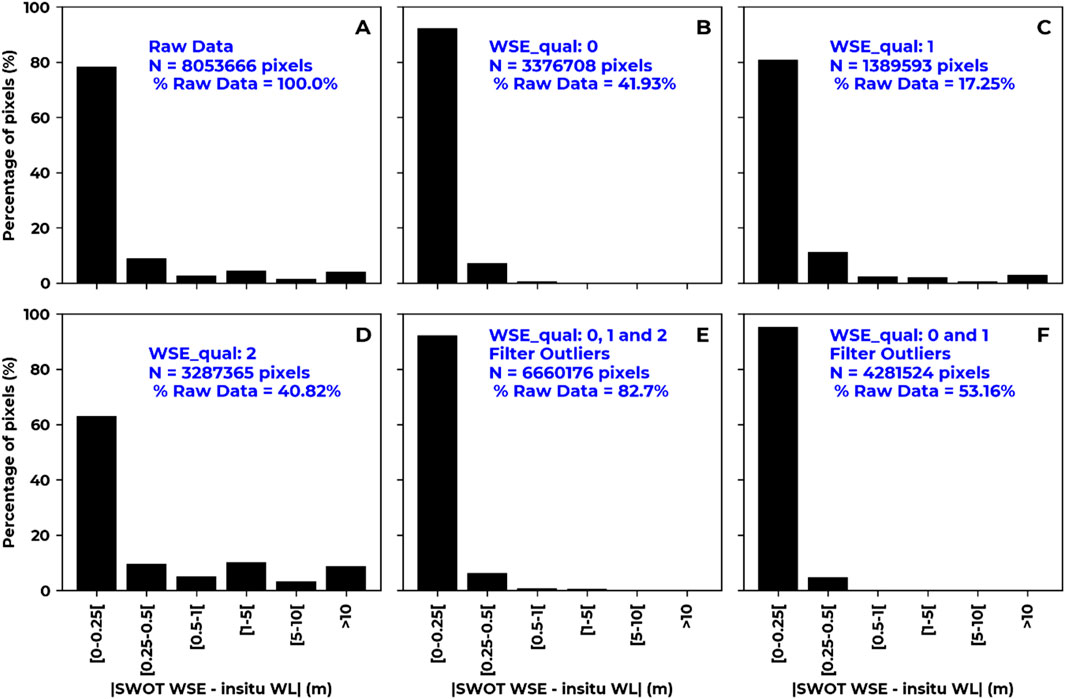
Figure 3. Distribution of the absolute difference between SWOT WSE and in situ water level for (A) all datasets, (B) pixels with WSE quality = 0, (C) pixels with WSE quality = 1, (D) pixels with WSE quality = 2, (E) pixels filtered by the outlier filter, and (F) pixels with WSE quality either 0 or 1 with outlier filter applied.

Applying the outlier filter (Section 3.2.1) while keeping all WSE_qual data (0, 1, and 2) maintains 82.7% of the whole dataset, with 92.3% of these pixels having an absolute difference of less than 25 cm and 6.3% having an absolute difference between 25 cm and 50 cm (Figure 3E). Only 1.4% of the pixels exhibit a high absolute difference between 50 cm and 5 m. These pixels could correspond to specific acquisition dates where most SWOT estimations (most of the grid cells) are abnormal and, thus, could not be detected as outliers by the MAD outlier filter. When considering only pixels with good (0) and suspect (1) qualities, followed by the application of the outlier filter, 53.16% of the data are retained, where 95.3% of these pixels showed an absolute difference of less than 25 cm, 4.7% showed an absolute difference between 25 and 50 cm, and no estimations exceeded an absolute difference of 50 cm (Figure 3F).

4.2 Overall SWOT elevation accuracy

Table 4 summarizes the accuracy metrics calculated for SWOT WSE compared to the in situ water level, considering different WSE quality flags with and without applying the outlier filter. Figure 4 shows the scatter plots of SWOT WSE vs. in situ water levels for four main configurations of Table 4. Data with good estimation quality (wse_qual = 0) showed an average difference (bias) of −0.09 m from in situ water levels with an RMSE of 0.19 m and an ubRMSE of 0.16 m. The correlation coefficient reached 0.8 for these pixels. However, the scatter plot in Figure 4A shows that for these pixels, some estimations may show significant differences (>1 m) from in situ measurements. Applying the outlier filter to these pixels with wse_qual = 0 slightly reduced the number of applicable pixels by 3.26% while reducing the RMSE by 6.1 cm to reach 0.13 m and increasing the correlation coefficient to reach 0.93 (Figure 4B). Pixels with suspected quality (wse_qual = 1) showed a very high bias, with RMSE, ubRMSE, and mean bias values reaching 6.18, 65.80, and 65.51 m, respectively. Removing outliers from these data significantly reduces the three metrics to −0.09, 0.13, and 0.09, respectively, while removing 2.56% of these points identified as outliers. Considering SWOT pixels with both good and suspect qualities (0 and 1) without filtering the outliers still results in large discrepancies compared to in situ water levels, with an RMSE of 35.53 m, a bias value of 1.73 m, and complete lack of correlation, with R dropping to 0. Similar results with very high RMSE and bias are shown when considering all the datasets with no quality control (wse_qual 0, 1, and 2). The outlier filter enhanced the accuracy metrics in both cases (wse_qual 0 and 1 or wse_qual 0, 1, and 2), where the RMSE reached 0.16 and 0.14 m, respectively, as shown in Table 4 and Figures 4C, D. However, considering all WSE qualities and applying the outlier filter still showed few anomalous estimations having differences from in situ water levels exceeding 1 m (scatter plot of Figure 4D). For the four scatter plots in Figure 4, many points appear as vertical lines compared to the in situ WL. Vertical lines in the scatter plot could be related to the availability of only one in situ WL measurement corresponding to all the SWOT grid cells (points) at each acquisition date, as mentioned in the methods section. This consideration could lead to vertical lines in the scatter plot, where we can obtain variable SWOT WSE estimations at a given date, compared to the same in situ WL at this date. However, the lake’s surface is generally flat, and the water levels are considered spatially uniform across its entire extent.

Table 4

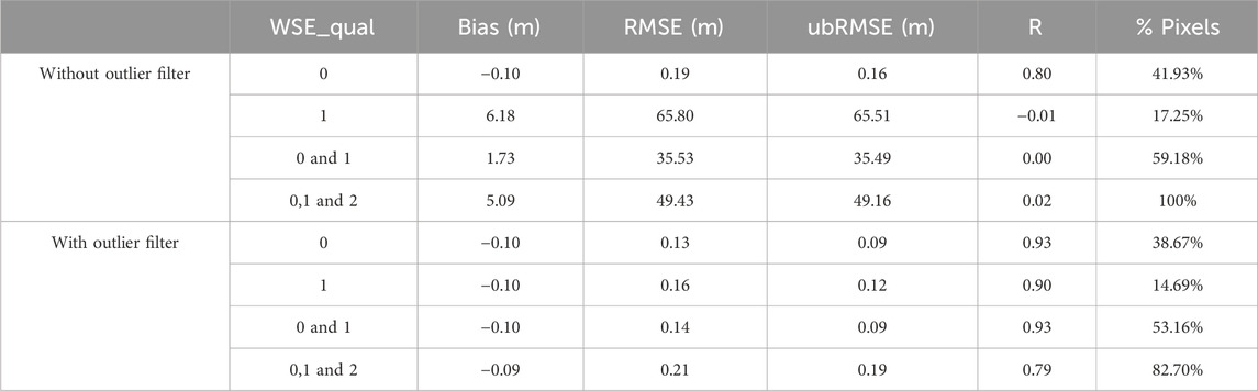
Table 4. Accuracy metrics of SWOT WSE computed for different WSE qualities with and without outlier filter.

Figure 4

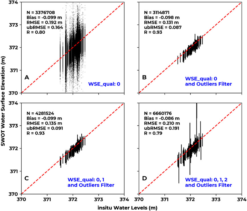
Figure 4. Scatter plot of in situ water levels and SWOT WSE for (A) data with good estimations (wse_qual = 0), (B) data with good estimation and outlier filter applied, (C) data with good (0) and suspect (1) estimations with outlier filter applied, and (D) data with all WSE qualities outlier filter applied.

4.3 SWOT elevation accuracy by date

The bias, RMSE, and ubRMSE values were calculated at each SWOT acquisition date. Figure 5 shows the three accuracy metrics per date for two configurations: first for data with all WSE qualities (0, 1, and 2) filtered for outliers (Figure 5a) and second for data with good (0) and suspect (1) qualities filtered for outliers (Figure 5b). For all WSE qualities with an outlier filter (Figure 5a), the bias values across most of the acquisition dates range between −5 cm and −18 cm. Some exceptions are present, such as the cases of 14/11/2023 and 23/12/2023, where bias values were positive and reached 60 cm and 1.9 m, respectively, despite applying the outlier filter. The same trend of bias is shown for the RMSE and ubRMSE, with homogeneous values across most acquisitions and ranging between 7 cm and 20 cm, except for the previously mentioned dates. For the second configuration, considering the good and suspect qualities and applying the outlier filter, the bias values range between −18 cm and −5 cm for almost all dates, except for 11/11/2023, showing a positive bias value of 17 cm. The RMSE and ubRMSE for this configuration seem homogeneous across dates, ranging from 7 cm to 21 cm for RMSE and from 4 to 13 cm for ubRMSE.

Figure 5

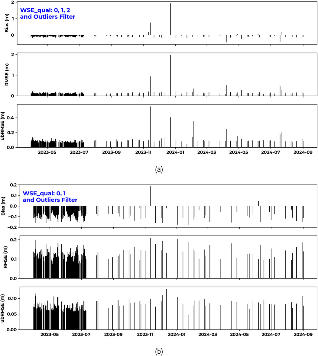
Figure 5. Bias, RMSE, and ubRMSE per SWOT acquisition date for (a) all WSE qualities with an outlier filter and (b) good (0) and suspect (1) SWOT WSE qualities with an outlier filter.

Figure 6 summarizes the results presented in Figure 5, showing the percentages of SWOT acquisitions (dates) for different ranges of the three accuracy metrics, namely, bias, RMSE, and ubRMSE for both the previously presented configurations in Figure 5. For the first configuration, results in Figure 6a showed that 80% of the SWOT acquisition dates had a bias value ranging between −15 cm and −5 cm. Only 1.5% of the dates had a bias value greater than 20 cm. For the RMSE, 61% of the SWOT dates had an RMSE between 10 and 15 cm and 21% had an RMSE between 15 and 20 cm. A total of 7% of the SWOT dates had an RMSE greater than 20 cm. The histogram of ubRMSE shows that 81% of the SWOT acquisition dates had an ubRMSE between 5 and 10 cm, 14% had an ubRMSE between 10 and 15 cm, and, finally, 3.5% had an ubRMSE greater than 20 cm. Comparable results are presented for the second configuration, considering only the good and suspect qualities (Figure 6b). For this configuration, the bias value does not exceed 20 cm, with no dates attaining a bias value greater than 20 cm. The ubRMSE for this configuration showed that 92% of the acquisition dates had an ubRMSE between 5 and 10 cm. However, using data with good and suspect qualities completely removes nine acquisition dates from the dataset (132 dates instead of 141 dates considering all WSE qualities), including the two dates of 14/11/2023 and 23/12/2023, which showed significant bias and RMSE in the first configuration. For all these nine dates, the WSE quality flag of all data (pixels) was equal to 2. However, retaining these bad quality data while applying the outlier filter resulted in reliable estimations for seven dates out of nine dates, preserving the continuity of the time-series. Only the cases of 14/11/2023 and 13/12/2023 remained with very high errors despite applying the outlier filter. These two dates are deeply analyzed and discussed further in the discussion section.

Figure 6

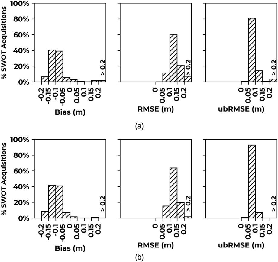
Figure 6. Percentage of SWOT acquisitions (dates) as a function of bias, RMSE, and ubRMSE using (a) data with all WSE qualities (0, 1, and 2) with outlier filter applied and (b) good and suspect SWOT WSE with outlier filter applied.

Figure 7 shows the time-series of the daily averaged SWOT WSE (black line) and the in situ water levels for the same two previously presented configurations (Figures 7A, B, respectively). The gray-shaded region represents the minimum and maximum boundaries calculated from the boxplot distribution at each acquisition date. For all WSE qualities and with the application of an outlier filter (Figure 7A), the two previously mentioned dates 14/11/2023 and 23/12/2023, with high bias and RMSE values, showed an average SWOT WSE exceeding the in situ water levels by 0.74 and 1.97 m, respectively. Regardless of these two dates for Figure 7A and despite the negative bias across most acquisition dates, Figures 7A, B show that the SWOT WSE estimations follow the trend and seasonality of the lake WSE. For Figure 7B, the measured WSE throughout the studied period from April 2023 to September 2024 varied by 0.97 m from 371.50 to 372.47 m. This variation in the lake water level is captured by the SWOT-estimated WSE, where both in situ measurements and SWOT estimates showed the same increasing and decreasing patterns. For example, from April 2023 to December 2023, the in situ water levels increased by 62 cm from an average of 371.73 m in April 2023 to 372.35 m in November 2023. A similar increase of 62 cm is obtained using SWOT with WSE varying from an average of 371.63 m in April 2023 to 372.25 m in December 2023. From December 2023 to April 2024, the in situ water level decreased by 78 cm from 372.35 m to reach a minimum of 371.57 in April 2024. The SWOT WSE showed the same decrease of 78 cm from 372.25 m in December 2023 to 371.46 m in April 2024. Generally, SWOT WSE showed a systematic constant negative bias of approximately −10 cm over the whole studied period. This constant bias value could be either due to a systematic error in the elevation extraction methods used by SWOT or could be related to the geoidal transformation errors due to the conversion of SWOT elevations to the same geoidal grid for the in situ data.

Figure 7

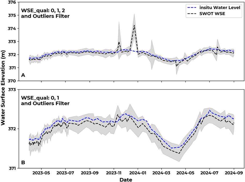
Figure 7. Time-series of SWOT WSE (black line) and in situ water levels (blue line) for (A) data with all WSE qualities with an outlier filter and (B) good and suspect SWOT WSE with an outlier filter. The gray-shaded region represents the minimum and maximum boundaries calculated from the boxplot distribution at each acquisition date.

5 Discussion

5.1 Explanation of SWOT WSE and in situ water level differences

We tried to analyze the differences between SWOT WSE and in situ water levels using the instrumental, atmospheric, and geophysical parameters associated with the WSE in the L2_HR_Raster. Some associated parameters include atmospheric variables such as, and not limited to, the sigma0 atmospheric attenuation (sig0_cor_atmos_model) or corrections due to delays from atmospheric propagation, i.e., ionosphere and dry and wet tropospheric delays (iono_corr, gim_ka, model_dry_tropo_cor, and model_wet_tropo_corrections). Other parameters are instrumental, such as the incidence angle, the cross-track, or the sigma0 values. Some parameters are related to geophysical corrections such as the tide heights (solid_earth_tide). All parameters (19 parameters in total) available in the L2_HR_Raster product were integrated into an RF model to explain the differences between SWOT WSE estimations and in situ water level measurements. All pixels from all dates were included in the RF regressor after considering WSE qualities of 0, 1, and 2 and applying the outlier filter. Data were randomly shuffled and split into 50% for training and 50% for validation. Assessing the feature importance in the explanatory random forest helps identify the variables that have the most significant impact on the difference between SWOT WSE and in situ water levels.

Figure 8 presents the feature importance in RF regression for all considered parameters. The parameter showing the highest importance in explaining the differences between SWOT and in situ water levels (0.44) appeared to be related to the dry tropospheric delay correction (model_dry_tropo_cor), followed by the atmospheric correction of the sigma0 values (sig0_cor_atmos_model) with a feature importance reaching 0.16. Cross-track values (distance between nadir and pixel positions related to the incidence angle) were ranked third, with an importance of approximately 0.07. Surface height displacement from load tide (load_tide_got) and ionospheric path delay correction had a contribution reaching approximately 0.06 and 0.04, respectively. The remaining parameters had no significant contribution as their importance dropped below 0.04.

Figure 8

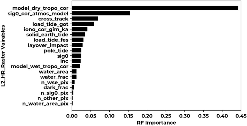
Figure 8. RF feature importance of the L2_HR_Raster parameters used to explain the difference between SWOT WSE and in situ water levels.

The dry tropospheric correction (DTC) applied to the SWOT grid points’ heights refers to the height’s corrections due to the propagation delay from the dry troposphere. This correction value was obtained from an independent SWOT information computed using the surface pressure from the European Center for Medium-Range Weather Forecasts (ECMWF) models. Several studies have reported the effect of tropospheric delays on interferometric height measurements (Doin et al., 2009; Yang et al., 2023). Correcting the propagation delays requires information on the surface pressure, which is usually estimated using weather models such as those from the ECMWF. Doin et al. (2009) reported that the average dry tropospheric delay over Lake Léman calculated using the ECMWF data ranges between −2.10 and −2.20 m, confirming the average value of the dry tropospheric correction in our dataset, which reached −2.20 m. However, in their study, they also report that this delay correction is subject to a standard deviation varying between 10 and 15 cm for our study site. In addition, the sigma0 atmospheric correction (sig0_cor_atmos_model) is a radiometric correction of sigma0 obtained from the numerical weather prediction model of the ECMWF. Contrary to the ocean case, where DTC is very accurate (1–2 cm), larger errors that occur over inland water due to interpolation errors of the correction derived from coarse resolution meteorological fields related to along-track effects were identified for nadir altimetry (Fernandes et al., 2014). This source of error also impacts wide-swath altimetry, affecting both along-track and across-track measurements due to similar interpolation issues. As highlighted by Mehran et al. (2017) regarding the wet tropospheric correction, meteorological model outputs cannot achieve sub-kilometric spatial resolution. Therefore, the two most significant variables affecting the SWOT WSE estimations are mainly related to atmospheric conditions affecting the backscattered sigma0 values and, thus, the heights’ estimations. Atmospheric perturbation could be the reason behind the highly visible errors for the date 14/11/2023 (Figures 5, 7). To understand the atmospheric perturbations or probably the meteorological conditions of this date, we analyzed the rainfall data derived from the ERA-5 (ECMWF reanalysis fifth generation) daily data for the whole studied period. Rainfall data showed that on 14/11/2023, a heavy rainfall event was encountered with a cumulative amount of 53 mm in 1 day. This value was the highest recorded rainfall event during the period between March 2023 and September 2024. As a direct effect of this rainfall event, in situ water levels showed an increase in the lake’s elevation by 35 cm between 11/11/2023 and 15/11/2023. This heavy rainfall condition could explain the heavily charged atmospheric conditions, leading to high perturbation in the SWOT sigma0 values and, thus, higher errors in the WSE estimations.

5.2 Effect of cross-track on SWOT accuracy

In this section, we analyze the effect of the SWOT cross-track on the accuracy of SWOT measurements as cross-track variations appear to impact SWOT WSE estimates, as shown by the variable importance in the RF model (Figure 8). Cross-track provides a signed distance (positive and negative) from the pixel to the spacecraft nadir point, where negative values indicate that the pixel is at the left side of the nadir. Cross-track and incidence angle are correlated, where low cross-track values (negative or positive) are near-nadir acquisitions with a low incidence angle and high absolute cross-track values are far-nadir acquisitions with a high incidence angle (in the right or left directions). Figure 9 shows the boxplots of the differences between SWOT WSE and in situ water levels for each 5 km range of cross-track values for three filtering configurations: (a) for data with good and suspect WSE qualities, (b) for data with all WSE qualities and an outlier filter, and (c) for data with only good WSE qualities. Over the lake, cross-track values varied from approximately −65 km (65 km to the left of the nadir) to 65 km to the right of the nadir. Figure 10 completes Figure 9 by showing the mean absolute difference for all pixels (data) for the same range of cross-tracks and the same three filtering configurations. For data with good and suspect qualities (Figure 9A), the boxplot shows that at nadir (cross-track between −5 and 0 km), large error values could be obtained ranging from −0.6 m to 0.6 m, and an absolute average error is shown in Figure 10A exceeding 10 m (the boxplot does not show outliers). The range of error values then starts to decrease as we move away sides from the nadir (both negative and positive cross-tracks), reaching a smaller variation at 25 and 30 km (on both sides) and an absolute difference decreasing to reach a value between 0.1 and 0.13 m for cross-tracks between 20 and 40 km. As we move far from the nadir with larger cross-track values greater than 50 km, the range of differences between SWOT and in situ expands and obtains a very large distribution (between −0.65 and 0.62) for very far cross-tracks exceeding 55 km on both sides. This pattern is valid in both directions, where the absolute difference for extreme cross-track values in Figure 10A also increases to reach 0.33 and 0.27 for the left and right directions, respectively.

Figure 9

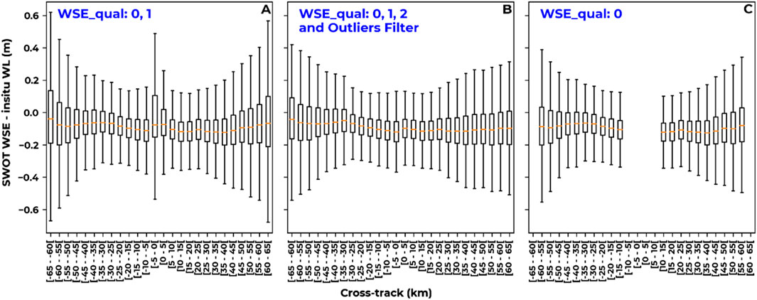
Figure 9. Boxplots of the difference (in m) between SWOT WSE and in situ water levels for ranges of cross-tracks in km for (A) SWOT data with good (0) and suspect (1) qualities without outlier filter, (B) all SWOT data with an outlier filter, and (C) SWOT data with good (0) WSE quality and no outlier filter.

Figure 10

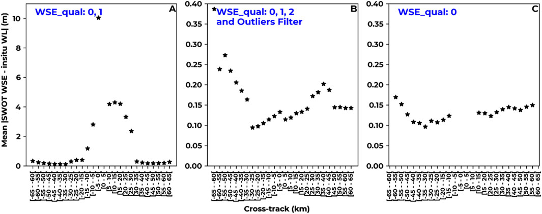
Figure 10. Mean absolute difference (in m) between SWOT and in situ water levels for ranges of cross-tracks in km for (A) data with good (0) and suspect (1) qualities, (B) all data qualities with an outlier filter, and (C) data with good (0) WSE quality.

Applying the outlier filter while preserving all WSE qualities (Figure 9B) significantly reduces the errors observed before at the nadir point (cross-track between −5 and 5 km), with an average absolute difference in Figure 10B reaching 13 cm. As observed before, the differences between SWOT WSE and in situ water levels decrease as move away from the nadir point in both directions but increase again at greater distances in both directions. While Figure 9B shows the boxplots expanding as we move farther, Figure 10B shows that for very high cross-track values on the left side of the nadir (>55 km), the absolute error increases to 38 cm compared to 9 cm at distances between −25 and −30 km from the nadir. The same pattern is observed for the data with only good WSE qualities, as shown in Figures 9C, 10C, except that the WSE quality filter for good data completely removes pixels at the nadir point (empty boxplots) and at a very high extent (−60 km and 60 km) from both sides. Removing these points decreased the mean absolute error to a range between 16 cm for high cross-tracks and 9 cm for near nadir cross-tracks (20–30 km).

The cross-track effect is highly visible for the date 23/12/2023, where high bias and RMSE values reaching approximately 2 m were observed (Figures 5A, 7A) for data with all WSE qualities and an outlier filter applied. The two maps in Figure 11, which represent cross-track values and WSE differences for 23 December 2023, show that while the cross-track values of this date ranged between −30 km and −60 km (with no nadir data and no positive cross-tracks), the differences between SWOT and in situ water levels reached 1 m for moderate cross-track values (−30 km) and gradually increased as the distance from the nadir grew, reaching approximately 2.85 m for far cross-tracks (<−60 km).

Figure 11

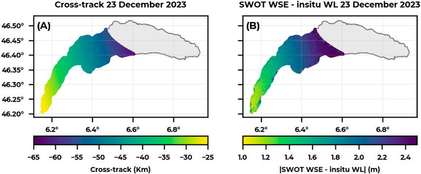
Figure 11. Example of high cross-track effect on SWOT WSE for 23 December 2023 showing (A) the cross-track map and (B) the absolute difference between SWOT WSE and in situ water levels considering WSE qualities 0, 1, and 2 with an outlier filter applied.

The effect of near-nadir measurements on WSE is presented in Figure 12, showing an example of unreliable nadir WSE on 13 April 2023 (the date is only an example among many similar ones). Despite considering only pixels of good (0) and suspect (1) qualities (such as the case of Figure 9A), which removed an important part of nadir pixels (the gray area on the map), some near-nadir measurements (cross-track near 0) still persist and show a high difference from in-situ WSE (between 4 and 10 m). This indicates that for such irrelevant remaining WSE, after being filtered by the WSE quality, the outlier filter could be a relevant solution to exclude such abrupt WSE estimations.

Figure 12

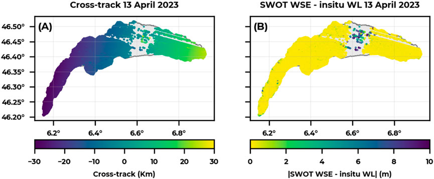
Figure 12. Example of the nadir effect on SWOT WSE on 13 March 2023 showing (A) the cross-track map and (B) the absolute difference between SWOT WSE and in situ water levels considering WSE qualities 0 and 1 without an outlier filter. The gray areas represent grid points where the SWOT WSE was filtered out due to quality filter.

5.3 Comparison with Sentinel-3, Sentinel-6, and GEDI altimetry-based water levels

In this section, we compared the SWOT accuracies to those obtained with competitor altimetry missions: S3A, S3B, S6, and GEDI. Table 5 summarizes the bias, RMSE, ubRMSE, and R obtained for each satellite mission. Since S3 and S6 data were obtained as unique daily measurements, the GEDI and SWOT acquisitions at each date were averaged for all tracks (GEDI) and pixels (SWOT), respectively, to obtain a unique daily value for each acquisition (see Section 3.3 in Methods), and the four accuracy metrics are calculated accordingly. For SWOT data, only pixels with good (0) and suspect (1) qualities were kept, and an outlier filter was applied before averaging the pixels’ values for each date. For GEDI data, the filters explained in Section 3.2.2 are applied before averaging. In terms of RMSE, SWOT and S3A appear to have comparable accuracies with an RMSE, reaching 11 and 13 cm, respectively. A slightly lower bias is achieved by SWOT (−0.09 m) than S3A. S3B had slightly lower accuracy than S3A and SWOT. The ubRMSE for S3A, S3B, and SWOT tend to have very low values not exceeding 4 cm, where both RMSE and bias showed nearly similar magnitudes. This indicates that the remaining error for the three missions could principally be a systematic error with relatively constant bias, probably related to either the geoid transformation of altitudes or a systematic error in the elevation estimation method used for each mission. S6 had the lowest accuracy compared to S3 and SWOT, with an RMSE reaching 20 cm. A positive bias was observed for S6, reaching 21 cm, whereas the ubRMSE still attained low values, probably showing the same systematic error as observed in S3 and SWOT. On the other hand, GEDI (LiDAR) data had the worst estimation compared to SAR missions. Using the GEDI acquisitions, the RMSE for the lake levels reached 49 cm (the highest obtained RMSE), with an overestimation of the lake’s elevations having a positive bias reaching 27 cm and an ubRMSE of 41 cm. The correlation coefficient for GEDI reached only 0.45 compared to 0.95 for S6, 0.98 for S3B and SWOT, and 0.99 for S3A.

Table 5

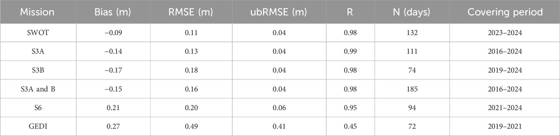
Table 5. Accuracy metrics in m for S3A, S3B, S6, GEDI, and SWOT on daily scale.

Figure 13 shows the time-series data of water surface elevations for all altimetric missions. Sentinel-3A and 3B were merged into a single time-series due to their similar accuracy metrics (Table 4). In Figure 13, both Sentinel-3 and SWOT better follow the trends and fluctuations of in situ water level variations compared to other missions. SWOT and Sentinel-3 provide closely matching, both exhibiting a slight underestimation throughout the whole period. The time-series of Sentinel-6 also follows the trends and fluctuations of the WSE well but exhibits a higher positive overestimation. On contrary, GEDI data showed the highest overestimation throughout the whole period of GEDI acquisitions, with noisier fluctuations compared to other missions; these fluctuations included negative and positive peaks that did not correspond to real in situ variations in the water level.

Figure 13

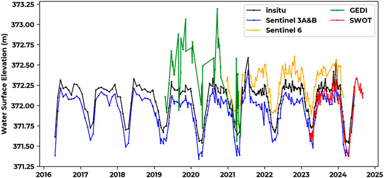
Figure 13. Time-series of water surface elevation from in situ measurements (black), Sentinel-3A and 3B estimations (blue), Sentinel-6 estimations (orange), GEDI elevations (green), and, finally, SWOT estimations (red).

6 Conclusion

This study evaluates the new SWOT mission for estimating WSEs over Lake Léman, Switzerland, using the level 2 (L2-HR-Raster) product. SWOT WSE data from the calibration and nominal phases were compared with in situ gauge stations and data from other similar altimetry missions, including S3A, S3B, S6, and GEDI LiDAR data. The main findings show that the RMSE between SWOT WSE and the in situ water levels ranged from 13 cm to 21 cm, depending on the measurement quality indicated by the L2-HR-Raster product’s WSE quality flag. A consistent bias of approximately −10 cm was observed across the WSE time-series, which could be attributed to geoidal transformation errors or systematic issues in the elevation extraction methods used by SWOT. The analysis also revealed that the nadir and near-nadir SWOT measurements were unreliable, with mean absolute differences from in situ water levels potentially exceeding 5 m. As a result, the study recommends that end-users apply a complementary outlier filter to eliminate unreliable WSE estimates rather than relying solely on the WSE quality flag. A random forest analysis of potential error sources in SWOT WSE revealed that atmospheric perturbation, particularly tropospheric delay, was the most significant factor affecting the accuracy of the measurements. Compared to other satellite altimetry missions, SWOT demonstrated the highest accuracy, achieving the lowest RMSE of 11 cm on a daily scale, compared to 13 cm for S3A, 18 cm for S3B, and 20 cm for S6. In contrast, GEDI LiDAR data had the least accuracy, with an RMSE of 46 cm and a bias of 27 cm.

Future research directions might include the analysis of the information contained in the SWOT Level 2 Water Mask Pixel Cloud Data Product (SWOT_L2_HR_PIXC) to improve the identification of valid water level estimates. Complementary information on the interferogram (e.g., coherent power and phase ambiguity), sensor baseline, layover, and spacecraft pith and roll could provide valuable insights for detecting outliers. In addition, the use of a higher spatial resolution product, with pixel sizes ranging from 10 to 60 m, would be of interest to better observe the areas close to the lake shores. Data merging with high-resolution satellite images (e.g., Sentinel-1 and 2 and NISAR in the near future) might also help in more accurately delineating lake shores and their temporal evolution to better quantify lake water storage.

Data availability statement

Publicly available datasets were analyzed in this study. These data can be found at: https://hydroweb.next.theia-land.

Author contributions

HB: conceptualization, data curation, formal analysis, investigation, methodology, software, visualization, writing – original draft, and writing – review and editing. NB: conceptualization, formal analysis, methodology, validation, and writing – review and editing. Y-NN: data curation and writing – review and editing. CN: data curation and writing – review and editing. FF: formal analysis, methodology, validation, and writing – review and editing. CC: data curation, formal analysis, validation, writing – review and editing.

Funding

The author(s) declare that financial support was received for the research and/or publication of this article. This research received funding from the French Space Study Center (CNES, TOSCA 2025 project) and the National Research Institute for Agriculture, Food, and the Environment (INRAE).

Conflict of interest

Author CC was employed by CS Group France.

The remaining authors declare that the research was conducted in the absence of any commercial or financial relationships that could be construed as a potential conflict of interest.

The author(s) declared that they were an editorial board member of Frontiers, at the time of submission. This had no impact on the peer review process and the final decision.

Generative AI statement

The author(s) declare that no Generative AI was used in the creation of this manuscript.

Publisher’s note

All claims expressed in this article are solely those of the authors and do not necessarily represent those of their affiliated organizations, or those of the publisher, the editors and the reviewers. Any product that may be evaluated in this article, or claim that may be made by its manufacturer, is not guaranteed or endorsed by the publisher.

References

Abdalla, S., Kolahchi, A. A., Ablain, M., Adusumilli, S., Bhowmick, S. A., Alou-Font, E., et al. (2021). Altimetry for the future: building on 25 years of progress. Adv. Space Res. 68, 319–363. doi:10.1016/j.asr.2021.01.022

CrossRef Full Text | Google Scholar

Alderman, K., Turner, L. R., and Tong, S. (2012). Floods and human health: a systematic review. Environ. Int. 47, 37–47. doi:10.1016/j.envint.2012.06.003

PubMed Abstract | CrossRef Full Text | Google Scholar

Aminjafari, S., Brown, I. A., Frappart, F., Papa, F., Blarel, F., Mayamey, F. V., et al. (2024). Distinctive patterns of water level change in Swedish lakes driven by climate and human regulation. Water Resour. Res. 60, e2023WR036160. doi:10.1029/2023WR036160

CrossRef Full Text | Google Scholar

Baron, J. S., Poff, N. L., Angermeier, P. L., Dahm, C. N., Gleick, P. H., Hairston, N. G., et al. (2002). Meeting ecological and societal needs for freshwater. Ecol. Appl. 12, 1247–1260. doi:10.1890/1051-0761(2002)012[1247:MEASNF]2.0.CO;2

CrossRef Full Text | Google Scholar

Baup, F., Frappart, F., and Maubant, J. (2014). Combining high-resolution satellite images and altimetry to estimate the volume of small lakes. Hydrol. Earth Syst. Sci. 18, 2007–2020. doi:10.5194/hess-18-2007-2014

CrossRef Full Text | Google Scholar

Biancamaria, S., Frappart, F., Leleu, A.-S., Marieu, V., Blumstein, D., Desjonquères, J.-D., et al. (2017). Satellite radar altimetry water elevations performance over a 200 m wide river: evaluation over the Garonne River. Adv. Space Res. 59, 128–146. doi:10.1016/j.asr.2016.10.008

CrossRef Full Text | Google Scholar

Biancamaria, S., Lettenmaier, D. P., and Pavelsky, T. M. (2016). “The SWOT mission and its capabilities for land hydrology,” in Remote sensing and water resources, space sciences series of ISSI. Editors A. Cazenave, N. Champollion, J. Benveniste, and J. Chen (Cham: Springer International Publishing), 117–147. doi:10.1007/978-3-319-32449-4_6

CrossRef Full Text | Google Scholar

Birkett, C. M. (1995). The contribution of TOPEX/POSEIDON to the global monitoring of climatically sensitive lakes. J. Geophys. Res. 100, 25179–25204. doi:10.1029/95JC02125

CrossRef Full Text | Google Scholar

Birkett, C. M. (1998). Contribution of the Topex Nasa Radar Altimeter to the global monitoring of large rivers and wetlands. Water Resour. Res. 34, 1223–1239. doi:10.1029/98WR00124

CrossRef Full Text | Google Scholar

Bogning, S., Frappart, F., Blarel, F., Niño, F., Mahé, G., Bricquet, J.-P., et al. (2018). Monitoring water levels and discharges using radar altimetry in an ungauged river basin: the case of the ogooué. Remote Sens. 10, 350. doi:10.3390/rs10020350

CrossRef Full Text | Google Scholar

Cheney, R. E. (2001). “Satellite altimetry,” in Encyclopedia of ocean sciences (Elsevier), 2504–2510. doi:10.1006/rwos.2001.0340

CrossRef Full Text | Google Scholar

Cretaux, J.-F., Calmant, S., Papa, F., Frappart, F., Paris, A., and Berge-Nguyen, M. (2023). Inland surface waters quantity monitored from remote sensing. Surv. Geophys 44, 1519–1552. doi:10.1007/s10712-023-09803-x

CrossRef Full Text | Google Scholar

de Fleury, M., Kergoat, L., and Grippa, M. (2023). Hydrological regime of sahelian small waterbodies from combined sentinel-2 MSI and sentinel-3 synthetic aperture radar altimeter data. Hydrology Earth Syst. Sci. 27, 2189–2204. doi:10.5194/hess-27-2189-2023

CrossRef Full Text | Google Scholar

Doin, M.-P., Lasserre, C., Peltzer, G., Cavalié, O., and Doubre, C. (2009). Corrections of stratified tropospheric delays in SAR interferometry: validation with global atmospheric models. J. Appl. Geophys. Adv. SAR Interferom. 2007 Fringe Workshop 69, 35–50. doi:10.1016/j.jappgeo.2009.03.010

CrossRef Full Text | Google Scholar

Dubayah, R., Blair, J. B., Goetz, S., Fatoyinbo, L., Hansen, M., Healey, S., et al. (2020). The global ecosystem dynamics investigation: high-resolution laser ranging of the Earth’s forests and topography. Sci. Remote Sens. 1, 100002. doi:10.1016/j.srs.2020.100002

CrossRef Full Text | Google Scholar

Dubayah, R., Hofton, M., Blair, J., Armston, J., Tang, H., and Luthcke, S. (2021a). GEDI L2A elevation and height metrics data global footprint level V002. doi:10.5067/GEDI/GEDI02_A.002

CrossRef Full Text | Google Scholar

Dubayah, R., Luthcke, S., Blair, J., Hofton, M., Armston, J., and Tang, H. (2021b). GEDI L1B geolocated waveform data global footprint level V002. doi:10.5067/GEDI/GEDI01_B.002

CrossRef Full Text | Google Scholar

Dudgeon, D., Arthington, A. H., Gessner, M. O., Kawabata, Z., Knowler, D. J., Lévêque, C., et al. (2006). Freshwater biodiversity: importance, threats, status and conservation challenges. Biol. Rev. 81, 163–182. doi:10.1017/S1464793105006950

PubMed Abstract | CrossRef Full Text | Google Scholar

Fayad, I., Baghdadi, N., Bailly, J.-S., Frappart, F., and Pantaleoni Reluy, N. (2022a). Correcting GEDI water level estimates for inland waterbodies using machine learning. Remote Sens. 14, 2361. doi:10.3390/rs14102361

CrossRef Full Text | Google Scholar

Fayad, I., Baghdadi, N., Bailly, J. S., Frappart, F., and Zribi, M. (2020). Analysis of GEDI elevation data accuracy for inland waterbodies altimetry. Remote Sens. 12, 2714. doi:10.3390/rs12172714

CrossRef Full Text | Google Scholar

Fayad, I., Baghdadi, N., and Frappart, F. (2022b). Comparative analysis of GEDI’s elevation accuracy from the first and second data product releases over inland waterbodies. Remote Sens. 14, 340. doi:10.3390/rs14020340

CrossRef Full Text | Google Scholar

Fernandes, M., Lázaro, C., Nunes, A., and Scharroo, R. (2014). Atmospheric corrections for altimetry studies over inland water. Remote Sens. 6, 4952–4997. doi:10.3390/rs6064952

CrossRef Full Text | Google Scholar

Fjortoft, R., Gaudin, J.-M., Pourthie, N., Lalaurie, J.-C., Mallet, A., Nouvel, J.-F., et al. (2014). KaRIn on SWOT: characteristics of near-nadir ka-band interferometric SAR imagery. IEEE Trans. Geosci. Remote Sens. 52, 2172–2185. doi:10.1109/TGRS.2013.2258402

CrossRef Full Text | Google Scholar

Frappart, F., Blarel, F., Fayad, I., Bergé-Nguyen, M., Crétaux, J.-F., Shu, S., et al. (2021). Evaluation of the performances of radar and lidar altimetry missions for water level retrievals in mountainous environment: the case of the Swiss lakes. Remote Sens. 13, 2196. doi:10.3390/rs13112196

CrossRef Full Text | Google Scholar

Fu, L., Pavelsky, T., Cretaux, J., Morrow, R., Farrar, J. T., Vaze, P., et al. (2024). The surface water and Ocean Topography mission: a breakthrough in radar remote sensing of the Ocean and land surface water. Geophys. Res. Lett. 51, e2023GL107652. doi:10.1029/2023GL107652

CrossRef Full Text | Google Scholar

Fuentes-Aguilera, P., Rodríguez-López, L., Bourrel, L., and Frappart, F. (2024). Recovery of time series of water volume in lake ranco (south Chile) through satellite altimetry and its relationship with climatic phenomena. Water 16, 1997. doi:10.3390/w16141997

CrossRef Full Text | Google Scholar

Höhle, J., and Höhle, M. (2009). Accuracy assessment of digital elevation models by means of robust statistical methods. ISPRS J. Photogrammetry Remote Sens. 64, 398–406. doi:10.1016/j.isprsjprs.2009.02.003

CrossRef Full Text | Google Scholar

Jiang, L., Andersen, O. B., Nielsen, K., Zhang, G., and Bauer-Gottwein, P. (2019). Influence of local geoid variation on water surface elevation estimates derived from multi-mission altimetry for Lake Namco. Remote Sens. Environ. 221, 65–79. doi:10.1016/j.rse.2018.11.004

CrossRef Full Text | Google Scholar

Kittel, C. M. M., Jiang, L., Tøttrup, C., and Bauer-Gottwein, P. (2021). Sentinel-3 radar altimetry for river monitoring – a catchment-scale evaluation of satellite water surface elevation from Sentinel-3A and Sentinel-3B. Hydrol. Earth Syst. Sci. 25, 333–357. doi:10.5194/hess-25-333-2021

CrossRef Full Text | Google Scholar

Kreibich, H., Van Loon, A. F., Schröter, K., Ward, P. J., Mazzoleni, M., Sairam, N., et al. (2022). The challenge of unprecedented floods and droughts in risk management. Nature 608, 80–86. doi:10.1038/s41586-022-04917-5

PubMed Abstract | CrossRef Full Text | Google Scholar

Leys, C., Ley, C., Klein, O., Bernard, P., and Licata, L. (2013). Detecting outliers: do not use standard deviation around the mean, use absolute deviation around the median. J. Exp. Soc. Psychol. 49, 764–766. doi:10.1016/j.jesp.2013.03.013

CrossRef Full Text | Google Scholar

Loizou, K., and Koutroulis, E. (2016). Water level sensing: state of the art review and performance evaluation of a low-cost measurement system. Measurement 89, 204–214. doi:10.1016/j.measurement.2016.04.019

CrossRef Full Text | Google Scholar

Maillard, P., Bercher, N., and Calmant, S. (2015). New processing approaches on the retrieval of water levels in Envisat and SARAL radar altimetry over rivers: a case study of the São Francisco River, Brazil. Remote Sens. Environ. 156, 226–241. doi:10.1016/j.rse.2014.09.027

CrossRef Full Text | Google Scholar

Mehran, A., Clark, E. A., and Lettenmaier, D. P. (2017). Spatial variability of wet troposphere delays over inland water bodies. JGR Atmos. 122. doi:10.1002/2017JD026525

CrossRef Full Text | Google Scholar

Merz, B., Blöschl, G., Vorogushyn, S., Dottori, F., Aerts, J. C. J. H., Bates, P., et al. (2021). Causes, impacts and patterns of disastrous river floods. Nat. Rev. Earth Environ. 2, 592–609. doi:10.1038/s43017-021-00195-3

CrossRef Full Text | Google Scholar

Nie, S., Wang, C., Li, G., Pan, F., Xi, X., and Luo, S. (2014). Signal-to-noise ratio–based quality assessment method for ICESat/GLAS waveform data. Opt. Eng. 53, 103104. doi:10.1117/1.OE.53.10.103104

CrossRef Full Text | Google Scholar

Nielsen, K., Stenseng, L., Andersen, O., and Knudsen, P. (2017). The performance and potentials of the CryoSat-2 SAR and SARIn modes for lake level estimation. Water 9, 374. doi:10.3390/w9060374

CrossRef Full Text | Google Scholar

Nilsson, B., and Nielsen, K. (2024). Validation of Sentinel-6MF based lake levels – an assessment with in situ data and other satellite altimetry data. Adv. Space Res. 73, 5806–5821. doi:10.1016/j.asr.2024.04.006

CrossRef Full Text | Google Scholar

Normandin, C., Frappart, F., Diepkilé, A. T., Marieu, V., Mougin, E., Blarel, F., et al. (2018). Evolution of the performances of radar altimetry missions from ERS-2 to sentinel-3A over the inner Niger delta. Remote Sens. 10, 833. doi:10.3390/rs10060833

CrossRef Full Text | Google Scholar

Oularé, S., Sokeng, V.-C. J., Kouamé, K. F., Komenan, C. A. K., Danumah, J. H., Mertens, B., et al. (2022). Contribution of sentinel-3A radar altimetry data to the study of the water level variations in lake buyo (west of côte d’Ivoire). Remote Sens. 14, 5602. doi:10.3390/rs14215602

CrossRef Full Text | Google Scholar

Papa, F., and Frappart, F. (2021). Surface water storage in rivers and wetlands derived from satellite observations: a review of current advances and future opportunities for hydrological sciences. Remote Sens. 13, 4162. doi:10.3390/rs13204162

CrossRef Full Text | Google Scholar

Pavlis, N. K., Holmes, S. A., Kenyon, S. C., and Factor, J. K. (2012). The development and evaluation of the EarthGravitational Model 2008 (EGM2008). J. Geophys. Res. 117, B04406. doi:10.1029/2011JB008916

CrossRef Full Text | Google Scholar

Pham-Duc, B., Frappart, F., Tran-Anh, Q., Si, S. T., Phan, H., Quoc, S. N., et al. (2022). Monitoring Lake volume variation from space using satellite observations—a case study in thac Mo reservoir (vietnam). Remote Sens. 14, 4023. doi:10.3390/rs14164023

CrossRef Full Text | Google Scholar

Reid, A. J., Carlson, A. K., Creed, I. F., Eliason, E. J., Gell, P. A., Johnson, P. T. J., et al. (2019). Emerging threats and persistent conservation challenges for freshwater biodiversity. Biol. Rev. 94, 849–873. doi:10.1111/brv.12480

PubMed Abstract | CrossRef Full Text | Google Scholar

Ryan, J. C., Smith, L. C., Cooley, S. W., Pitcher, L. H., and Pavelsky, T. M. (2020). Global characterization of inland water reservoirs using ICESat-2 altimetry and climate reanalysis. Geophys. Res. Lett. 47, e2020GL088543. doi:10.1029/2020GL088543

CrossRef Full Text | Google Scholar

Shiklomanov, A. I., Lammers, R. B., and Vörösmarty, C. J. (2002). Widespread decline in hydrological monitoring threatens Pan-Arctic Research. EoS Trans. 83, 13–17. doi:10.1029/2002EO000007

CrossRef Full Text | Google Scholar

Shu, S., Liu, H., Beck, R. A., Frappart, F., Korhonen, J., Lan, M., et al. (2021). Evaluation of historic and operational satellite radar altimetry missions for constructing consistent long-term lake water level records. Hydrology Earth Syst. Sci. 25, 1643–1670. doi:10.5194/hess-25-1643-2021

CrossRef Full Text | Google Scholar

Søndergaard, M., and Jeppesen, E. (2007). Anthropogenic impacts on lake and stream ecosystems, and approaches to restoration. J. Appl. Ecol. 44, 1089–1094. doi:10.1111/j.1365-2664.2007.01426.x

CrossRef Full Text | Google Scholar

Sulistioadi, Y. B., Tseng, K.-H., Shum, C. K., Hidayat, H., Sumaryono, M., Suhardiman, A., et al. (2015). Satellite radar altimetry for monitoring small rivers and lakes in Indonesia. Hydrol. Earth Syst. Sci. 19, 341–359. doi:10.5194/hess-19-341-2015

CrossRef Full Text | Google Scholar

SWOT. (2024). SWOT level 2 water Mask raster image data product. doi:10.5067/SWOT-RASTER-2.0

CrossRef Full Text | Google Scholar

Wilcox, R. R. (2005). “Introduction to robust estimation and hypothesis testing,” in Statistical modeling and decision science. 2nd ed. Amsterdam: Elsevier/Academic Press.

Google Scholar

Xiang, J., Li, H., Zhao, J., Cai, X., and Li, P. (2021). Inland water level measurement from spaceborne laser altimetry: validation and comparison of three missions over the Great Lakes and lower Mississippi River. J. Hydrology 597, 126312. doi:10.1016/j.jhydrol.2021.126312

CrossRef Full Text | Google Scholar

Xu, J., Xia, M., Ferreira, V. G., Wang, D., and Liu, C. (2024). Estimating and assessing monthly water level changes of reservoirs and lakes in jiangsu province using sentinel-3 radar altimetry data. Remote Sens. 16, 808. doi:10.3390/rs16050808

CrossRef Full Text | Google Scholar

Yang, Q., Zuo, X., Guo, S., and Zhao, Y. (2023). Evaluation of InSAR tropospheric delay correction methods in the plateau monsoon climate region considering spatial–temporal variability. Sensors 23, 9574. doi:10.3390/s23239574

PubMed Abstract | CrossRef Full Text | Google Scholar

Yuan, C., Gong, P., and Bai, Y. (2020). Performance assessment of ICESat-2 laser altimeter data for water-level measurement over lakes and reservoirs in China. Remote Sens. 12, 770. doi:10.3390/rs12050770

CrossRef Full Text | Google Scholar

Zhang, G., Chen, W., and Xie, H. (2019). Tibetan plateau’s lake level and volume changes from NASA’s ICESat/ICESat-2 and landsat missions. Geophys. Res. Lett. 46, 13107–13118. doi:10.1029/2019GL085032

CrossRef Full Text | Google Scholar