Monitoring soil degradation using Sentinel-2 imagery and statistical analysis of spectral indices in a semi-arid watershed of the Moroccan High Atlas

The existence of serious water erosion problems in different parts of a watershed is often evidenced by the presence of high levels of suspended sediment in watercourses. The indirect assessment of erosion through the measurement of suspended sediments transported to catchment outlets serves as a robust indicator of the environmental impact of agricultural practices. The aim of this study is to propose a model for assessing the risk of soil degradation in the upstream Tassaoute watershed (in the Moroccan High Atlas). The methodology is based on the statistical analysis of spectral indices derived from Sentinel-2A satellite images acquired during the year 2021, including four vegetation indices and nine soil indices. These indices are aggregated to form a composite image (the independent variable), which is then subjected to regression analysis against the individual indices (the dependent variable) to determine correlation coefficients and coefficients of determination. Principal Component Analysis (PCA) is then used to condense the information from all the spectral indices, providing factorial coordinates and facilitating the identification of positive and negative correlations. The principal component captures soil-related information, while the secondary component focuses on vegetation characteristics. The final predictive model is developed by assigning weights to each index based on its coefficient of determination and the coordinates of the factors. This approach produces a quantitative map delineating four categories of soil potentially at risk of degradation. The results show that incorporating the spectral bands of Sentinel-2A’s C-MSI sensor into the calculation considerably improves accuracy and provides an accurate representation of ground reality.

1 Introduction

Soil erosion, recognized worldwide as the main form of land degradation, is intensified by the dynamic forces of water and wind, as well as by human activities such as grazing, farming, land clearing and land development for housing. These practices accelerate erosion. Erosion takes various forms, including intercalary erosion, sheet erosion, gully erosion and river erosion (1). Water-related soil erosion represents a critical environmental challenge and is a subject of major interest to researchers in various scientific fields such as pedology, geomorphology and forestry. It also represents a major environmental and agricultural risk (2). Interesting statistics from several research studies indicate that soil erosion affects more than 10 million hectares of farmland worldwide every year, with annual loss rates of around 43 petagrams (Pg) (3). A report by the FAO and the IAEA, published in January 2023, reveals that 1.9 billion hectares are currently affected by soil degradation, representing around 65% of the planet’s soils. Erosion alone accounts for 85% of this degradation. Around a quarter of the world’s population, or 1.5 billion people, depend directly on already degraded agricultural land. Every year, more than 36 billion tons of fertile soil are lost. The costs, for both cultivated and uncultivated land, are immense, reaching around 400 billion dollars a year (4, 5).

In the face of this crisis, erosion – particularly soil erosion caused by water – is attracting increasing attention from researchers and land management specialists. The loss of arable land is intensifying, threatening the sustainability of agricultural systems and the security of human infrastructures (1). To anticipate and minimize damage, it is essential to better understand the factors that influence these dynamics: rainfall patterns, soil types, topography and land use. This is why the study of erosion calls on a variety of disciplines, including physical geography, pedology, hydrology, engineering, human sciences and economics – a resolutely multidisciplinary approach (6). Soil erosion by water is a major factor in the transfer of sediment into rivers, poses a serious threat to land quality and affects around one billion hectares worldwide (7). It has impacts either on-site in the depletion of soil resources, reduced soil fertility, reduced vegetation growth, siltation of valleys and reservoirs, desertification and damage to human infrastructure or off-site include sedimentation in watercourses, reduced water quality, economic and ecological damage to communities (8, 9).

In Morocco, soil erosion affects 40% of the land, with annual loss rates ranging from 23 to 55 t/ha and reaching up to 524 t/ha in some regions (10, 11). And in terms of water erosion, each year Morocco causes soil losses ranging from 500 to over 5,000 t/km², depending on the region, and siltation of dam reservoirs to the tune of 75 million m³. This represents an annual reduction of around 0.5% in their storage capacity, resulting in a significant loss of water for irrigation of 10,000 ha/year, and a deterioration in the quality of available drinking water (according to data from the Moroccan High Commission for Water and Forests) (12–14). In Morocco’s watersheds, for example, specific erosion levels vary considerably from region to region. The highest rates, more than 2000 t/km²/year, are recorded in the Martil, Ouergha, Akhdar and Tassaout basins. Intermediate levels, between 1000 and 2000 t/km²/year, are found in the Neckor, M’Harhar and Loukkos basins. Other areas, such as the Sebou, Inanouène, Oued El Abid and Massa basins, have rates ranging from 500 to 1000 t/km²/year. The rest of the country has specific losses of less than 500 t/km²/year (15). Against this backdrop, Morocco is facing a growing water shortage, aggravated by pollution and the effects of climate change, and is in a situation of water stress, with an annual potential of 22 billion m³, or around 750 m³ per inhabitant, a level below the critical threshold of 1,000 m³/inhabitant/year. This scarcity represents a major environmental and socio-economic challenge, calling for rigorous and sustainable management of water resources (16, 17). In addition, agriculture is the main means of subsistence for the inhabitants of Morocco’s mountainous regions, which are heavily affected by soil erosion. This leads to a reduction in fertile land, a decline in water quality and availability, and a series of serious economic and social repercussions (18).

Given the complexity of this phenomenon, analysis methods have diversified according to spatial and temporal scales and objectives (6, 19). This diversity of models is linked to the complexity of the factors (precipitation, topography, soil properties, land use and land cover dynamics (LULC)) that control soil erosion, as well as to their variability in time and space. The study of water erosion has long relied on classical approaches, structured around empirical, conceptual, physical or statistical models. Each of these methods has advantages, but also limitations that restrict their applicability on a large scale or in heterogeneous environments. Empirical models, such as USLE (Universal Sol Loss Equation) or RUSLE (Revised USLE), offer a rapid estimate of sheet erosion, but their limited ability to be transposed to other contexts limits their effectiveness (20). Conceptual models, such as AGNPS (AGricultural Non-Point Source pollution model), provide a simplified representation of processes, but can accumulate uncertainties linked to the structuring of the model (21). As for physical models, such as WEPP (Water Erosion Prediction Project) or EUROSEM (European Soil Erosion Model), they provide detailed results but require a large volume of data, which is often difficult to obtain, and struggle to convey the true complexity of slopes (22). Finally, conventional statistical approaches remain limited by their sensitivity to the subjective choices of experts and their difficulty in integrating temporal dynamics (21).

In this context, modern approaches combining remote sensing and GIS Thanks to satellite imagery (MODIS, Landsat, Sentinel) to assess soil loss rates and risks, as the synergy between remote sensing and GIS has shown significant advantages in characterizing soil degradation over large territories with reasonable costs and ensuring good accuracy (21, 23). As with empirical–statistical approaches, the aim is to couple spectral indices with statistical analyses to distinguish and characterize, in an indirect but relevant way, the factors linked to soil erosion, while considerably reducing dependence on field data, which is often limited and costly to collect. As a result, spectral indices are emerging as effective indicators for discriminating levels of soil degradation and analyzing erosive dynamics in an efficient manner (24).

This study focuses on a semi-arid watershed in the Moroccan High Atlas, the upstream Tassaoute watershed, chosen because it has been subject to major hydro-agricultural developments, leading to a significant expansion of irrigated agricultural activities. These human interventions have profoundly altered the hydrological functioning of the river, directly impacting the filling process of the Moulay Youssef dam (25). The aim of this study is therefore to assess soil degradation in the upstream Tassaoute watershed using advanced analysis tools. The use of Sentinel-2A images due to their high spatial resolution and ability to capture multiple spectral bands and the combination of spectral indices as well as statistical analysis techniques to characterize soil properties and identify areas vulnerable to water erosion. This assessment relies on the exploitation of vegetation and soil indices to establish meaningful relationships between these parameters and degradation processes. The study also aims to provide an in-depth analysis of the factors influencing water erosion in the region. The results of this approach can provide basin managers with useful tools for implementing more appropriate soil and water conservation policies.

A central question is how to assess soil vulnerability to water erosion in the upstream Tassaoute watershed, using geospatial tools, spectral analysis and statistical analysis?

2 Materials and methods

2.1 Study area

The Tassaout watershed, located upstream of the Moulay Youssef artificial reservoir in the Central High Atlas region (south-eastern part of the Oum Er-Rbia basin). It covers an area of 1,418.35 km², with geographical coordinates ranging from latitudes 31°33’56 “N and 31°64’47” N, to longitudes 6°48’40” W and 7°33’40” W. This watershed is part of the northern sub-atlasic region known as the Demnate Atlas and lies to the east of the Haouz plain (Figure 1). It is around 35 km from the town of Demnate and 90 km from Marrakech. It is crossed by the Oued Tassaoute, whose source lies at an altitude of around 3,978 meters. Its course runs north-east to north-west, making it the main tributary of the Oued Oum Er-Rbia, which plays a major hydrological role in the region. The watershed is composed of pre-Permian sedimentary and metamorphic rocks, as well as the Jurassic massif to the east of Azilal (13, 26). This basin was chosen because of its specific characteristics: a semi-arid climate marked by irregular and stormy rainfall, rugged relief, degraded vegetation cover and a wealth of friable lithological formations. These characteristics contribute to increased soil degradation and loss of fertility, with often irreversible socio-economic and ecological impacts (13, 27). The basin is subdivided into two sub-basins, Ait Tamlil and Tamsemat, each with its own surface area and natural and anthropogenic characteristics, these basins are also characterized by significant flood runoff, representing 60% for the Tassaoute basin and 36% for the Ait Tamlil and Tamsemat sub-basins (25).

Figure 1

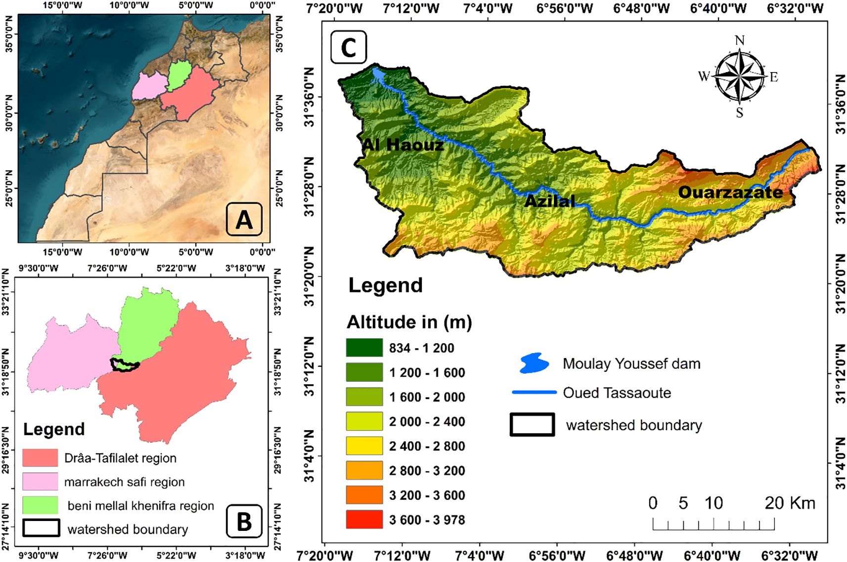
Figure 1. Location map. (A) Morocco, (B) Regions, (C) Upstream Tassaoute watershed.

2.2 Satellite data

The methodology is based on the use of Sentinel-2A images equipped with a high-resolution multi-spectral sensor called C-MSI (Capteur-Multi-Spectral Instrument). This sensor collects data in different spectral bands, from the visible to the near infrared, with a spatial resolution ranging from 10 meters to 60 meters, depending on the spectral band. The most used bands, such as red, green and blue, have a resolution of 10 meters, while the near-infrared bands have a resolution of 10 and 20 meters (28) (Table 1). The images used have a resolution of 10 meters and cover the period from August 1, 2021, to September 30, 2021.

Table 1

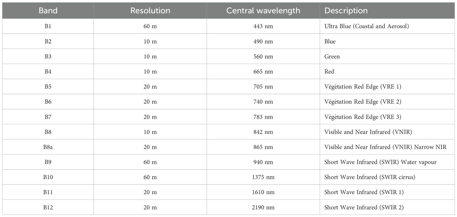
Table 1. Spectral bands of the C-MSI instrument on board Sentinel-2A.

Spectral index calculation and statistical analysis are performed with Google Earth Engine, using JavaScript scripts. This powerful geospatial data analysis platform provides access to a vast library of satellite images, including those from the Sentinel-2A satellite, facilitating the calculation of vegetation indices, as well as soil indices.

2.3 Modelling soil degradation

The methodology consists of calculating spectral indices derived from Sentinel-2A satellite imagery. Specifically, four vegetation indices are used: Normalized Difference Vegetation Index (NDVI), Modified Soil-Adjusted Vegetation Index 2 (MSAVI2), Disease Water Stress Index (DSWI) and Normalized Difference Greenness Index (NDGI). In addition, nine soil indices are calculated, including Moisture Stress Index (MSI), Texture Index (TI), Color Index (IC), Brightness Index (BI), Crust Index (CI), Grain Size Index (GSI), Encrustation Index (EI), Redness Index (RI) and Normalized Difference Salinity Index (NDSI). These indices are merged to form a synthesis image, which provides an integrated representation of the surface condition, offering global information relevant to the study of water erosion risk. Indeed, each index used has a specific ecological significance; however, no single index can fully characterize the erosion phenomenon. It is therefore both logical and necessary to combine them to obtain a completer and more coherent picture of soil condition. On the one hand, dense vegetation acts as a protective barrier against erosion, while bare or water-stressed soil becomes more vulnerable. On the other hand, the soil’s physico-chemical properties – such as texture, moisture, salinity, gloss, color and surface structure – directly influence its susceptibility to erosion, by conditioning key processes such as infiltration, runoff and particle cohesion (29, 30).

This is followed by a statistical analysis, which includes a linear regression analysis against the individual indices (the dependent variable) and a synthetic image to determine the correlation and determination coefficients. In addition, a principal component analysis (PCA) is performed to condense the information from all spectral indices, facilitating the identification of positive and negative correlations and the extraction of factorial coordinates the final step involves proposing an equation for the model, derived by assigning weights to each index based on its coefficient of determination and factorial coordinates, in order to predict the risk of soil degradation (Figure 2).

Figure 2

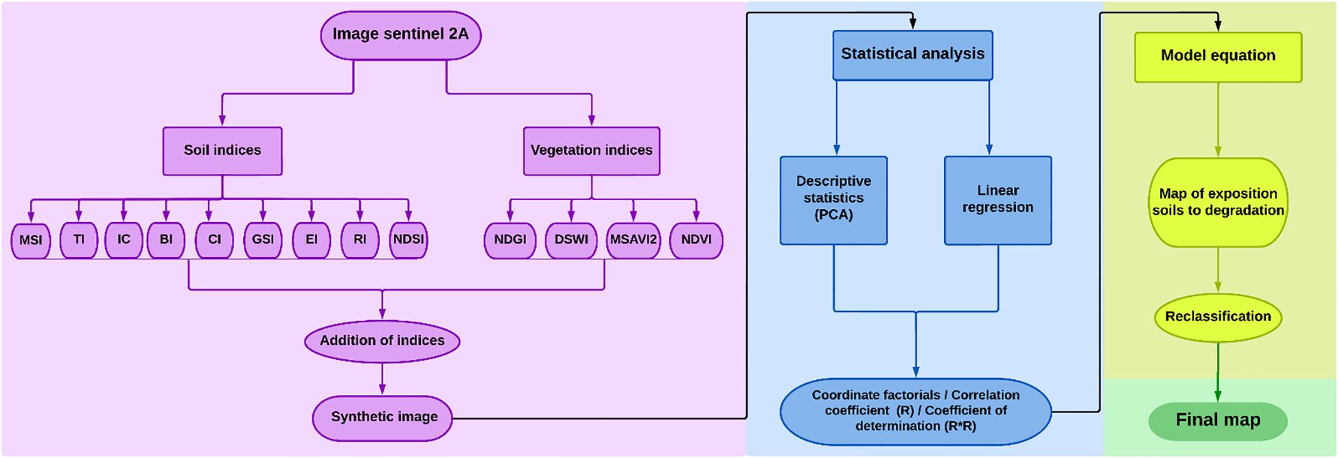
Figure 2. Flow chart of the adopted methodology.

2.4 Index modeling

2.4.1 Vegetation indices

Vegetation indices play a key role in assessing vegetation condition and its influence on soil erosion processes (31). In addition, their use has many benefits and applications, notably in estimating vegetation cover, monitoring plant health, tracking crop growth, assessing the quality of aquatic ecosystems, analyzing environmental change, climate modeling and forecasting agricultural yields (32) (Table 2).

Table 2

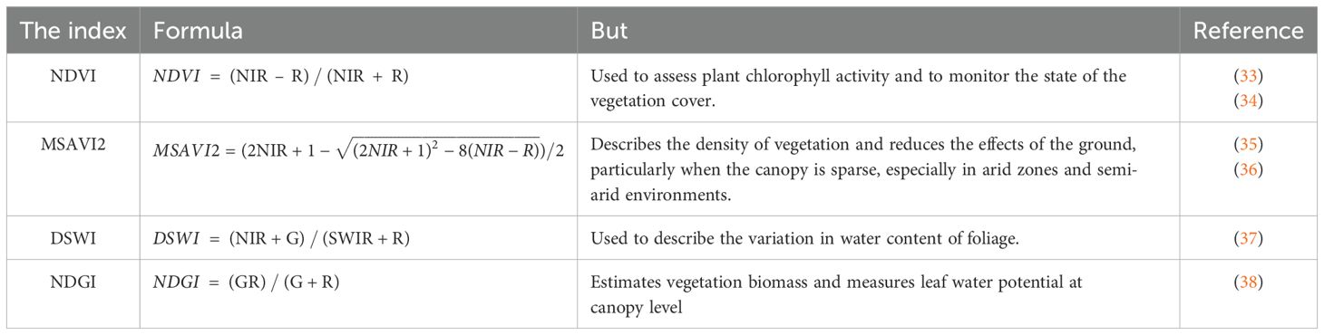
Table 2. Vegetation indices used in our method.

2.4.2 Soil indices

Soil indices (Table 3) are used to assess soil characteristics and properties from satellite data. They are based on the spectral responses of soils in different bands of the electromagnetic spectrum (47). The indices used characterize various soil properties, including water content, texture, fertility, mineralogical composition and organic matter content. They also provide valuable information on the physical state of the soil, particularly in terms of moisture and compactness. In addition, parameters such as color, luminosity and humidity are essential for mapping the absorption capacities of soil constituents, particularly in arid environments. This information is fundamental for rational agricultural land management, urban planning, natural resource conservation and sustainable development decision-making (41).

Table 3

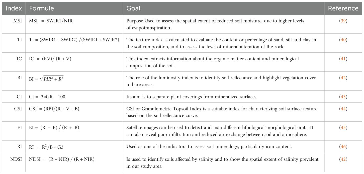
Table 3. Soil indices used in our method.

2.5 Statistical models

The model currently being developed also depends on statistical information extracted from the indices. This includes linear regression and PCA.

2.5.1 Linear regression

Linear regression analysis is a statistical technique for estimating the relationship between variables that have a reason–outcome relationship. The main objective of univariate regression is to analyze the relationship between a dependent variable and an independent variable, and to formulate the linear relationship equation between the dependent variable and the independent variable. Regression models with one dependent variable and several independent variables are called multilinear regression (48). In this study, we have the multilinear regression analysis a synthetic image serves as the explanatory variable, while spectral indices, such as vegetation and soil indices, represent the variables to be explained. This method is based on the idea that the relationship between variables can be approximated by a linear equation. The main objective of linear regression is to determine the coefficients of this equation, which quantify the effect of the explanatory variable on the variables to be explained. By analyzing how variations in a synthetic image affect vegetation and soil indices, linear regression can help identify significant trends and make forecasts.

The results of this analysis include important statistics, such as the determination coefficient (R²), which indicates the proportion of the variance in the variables to be explained that is captured by the model. In addition, statistical significance tests associated with the coefficients help to assess the relevance of the relationships identified (49).

2.5.2 Principal component analysis

PCA is a mathematical transformation commonly used in remote sensing. It is a multivariate analysis method that enables many variables to be studied simultaneously. When working in a space with more than three dimensions, visualizing all the information becomes difficult, if not impossible. PCA makes it possible to reduce this complexity, while highlighting relationships between variables and underlying phenomena (50, 51).

The aim of PCA is to concentrate information on a reduced number of axes, to identify the descriptors most strongly correlated with activities (52).

For this step, we use PCA, a powerful tool for synthesizing information and reducing the dimensional space of data. This statistical technique explores the structure of multidimensional data by transforming the original variables into a set of synthetic variables called “principal components” (53).

PCA results are presented in graphical form, supported by characteristic numerical values that facilitate interpretation. These graphs include geographical representations and tables, allowing us to observe the similarities and oppositions between the characteristics studied in relation to the various factors.

2.6 The equation proposed for the model

The model equation proposed here is designed to balance all the information obtained from the statistical analysis performed with the indices and based on previous working approaches (27):

RISQUE DE DEGRADATION DES SOLS = NDVI*(xmax+Ymax) *R² + MSAVI2*(xmax+Ymax) *R² + DSWI*(xmax+Ymax) *R² + NDGI*(xmax+Ymax) *R²+ MSI*(xmax+Ymax) *R² + BI *(xmax+Ymax) *R² + EI*(xmax+Ymax) *R² + TI*(xmax+Ymax) *R² + CI *(xmax+Ymax) *R² + RI*(xmax+Ymax) *R² + IC*(xmax+Ymax) *R² + GSI*(xmax+Ymax) *R² + NDSI*(xmax+Ymax) *R²

The R² therefore reflects the explanatory capacity of each index. The higher the R² value, the more relevant the index is in explaining erosion.

Factor coordinates are not simply statistical values. For example, if a soil index has a high coordinate on Dim1, this means it is strongly linked to the dominant variability structure between the data, often linked to physical or chemical soil degradation. If a vegetation index is strongly projected in opposition to these indices on the same axis, this may indicate a mitigating or protective role against erosion. These coordinates also determine whether an index has a positive or negative influence on the phenomenon under study.

So, the combined use of R² and factorial coordinates strengthens the reliability of the model. The R² is used to quantify predictive significance, while the factorial coordinates provide information on the meaning and structure of the information in the dataset, making it possible to distinguish erosion-aggravating factors from protective factors, depending on the direction of their projection. An optimal approach is to multiply each index by its spatial value, its R² and its factorial coordinate. Integrating these two elements into a spatial equation applied pixel by pixel (x, y) enables us to construct a robust and interpretable final map, synthesizing both statistical information and the geographical logic of soil degradation processes (50).

3 Results

3.1 Spectral indices

3.1.1 Vegetation indices

Analysis of the watershed reveals a predominance of medium- to low-density vegetation cover, reflecting a notable ecological fragility. Remote sensing indices such as NDVI, MSAVI2, DSWI and NDGI (Figure 3) confirm this trend, revealing sparse vegetation, reduced biomass and low leaf water content over most of the basin. These conditions accentuate vulnerability to water erosion, as vegetation plays an essential role in soil stabilization and runoff regulation. Although some localized areas have denser, healthier vegetation, as detected by high NDGI values, they remain limited in surface area. Taken together, these observations underline the need to step up efforts in sustainable land management and ecological restoration, to preserve natural resources and limit the impact of erosion in this region.

Figure 3

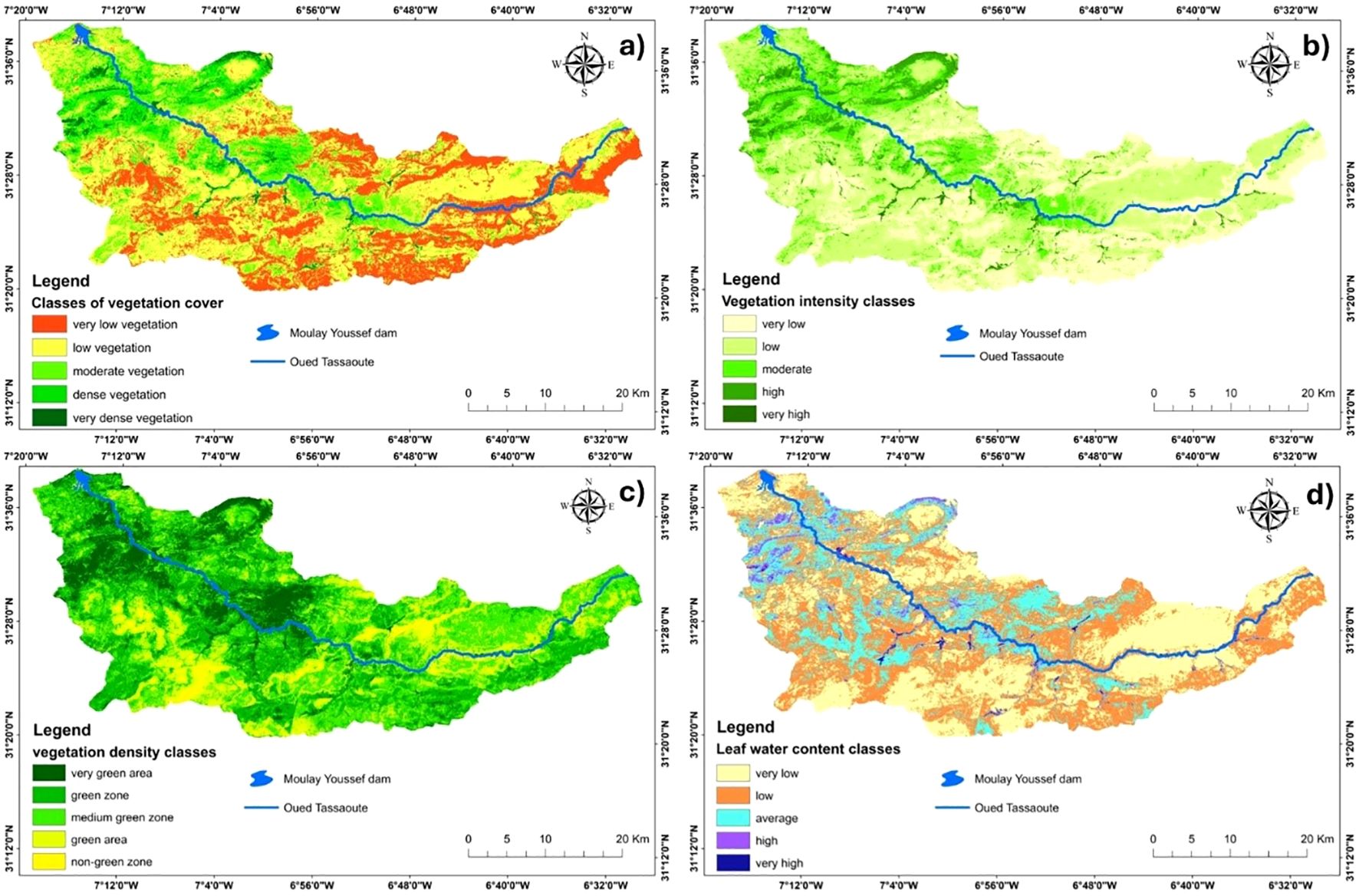
Figure 3. Vegetation index maps. (a) NDVI, (b) MSAVI2, (c) DSWI, (d) NDGI.

3.1.2 Soil indices

Analysis of nine soil indices in the study basin reveals a marked heterogeneity of soil characteristics, indicative of complex environmental dynamics. Maps derived from indices (Figure 4) such as MSI, TI, CI, BI, CI, GSI, EI, RI and NDSI provide a spatial diagnosis of soil constraints.

Figure 4

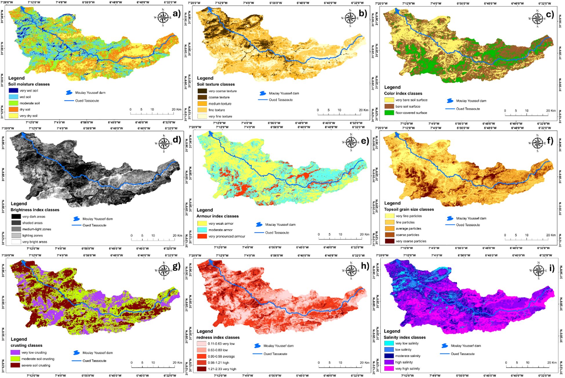
Figure 4. Soil index maps. (a) MSI, (b) TI, (c) IC, (d) BI, (e) CI, (f) GSI, (g) EI, (h) RI, (i) NDSI.

The results show a predominance of low-moisture soils, reflecting significant water stress. Texture classes indicate a predominance of medium to fine textured soils, likely to favor erosion in the case of low organic matter content. Color Index and Brightness Index reveal a predominance of bare to moderately dark surfaces, reflecting both low vegetation cover and exposure to erosion processes. CI reveals a significant occurrence of moderate to severe crusting, accentuating susceptibility to water erosion by limiting infiltration. In addition, GSI reveals the presence of course to very coarse particles in several areas, amplifying runoff. RI and EI show locally intense mineralization and marked leaching, testifying to the chemical alteration and ongoing erosion of surface horizons. Lastly, NDSI indicates salinity variability, with several areas showing moderate to high salinity, constituting an additional constraint for vegetation and agricultural uses.

All in all, these indices confirm the high vulnerability of the soils, linked to water scarcity, fragile structure, driving crust and salinity. These factors underline the need for an integrated soil management strategy based on conserving vegetation cover, combating runoff and restoring the physical and chemical properties of soils, with a view to strengthening the ecological resilience of the watershed.

3.2 Statistical analysis

3.2.1 Linear regression

The results of our analysis are illustrated in the figure below (Figure 5). By combining all the indices, we have generated a new image that synthesizes all the information provided by each index.

Figure 5

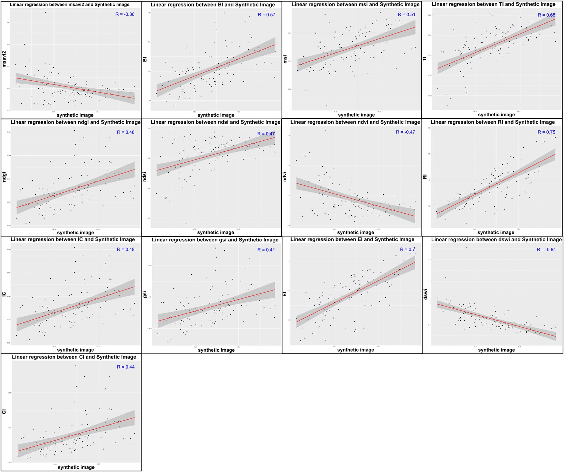
Figure 5. Correlation graphs between synthetic image and indices used.

Linear regression analysis was used to assess the relationship between the various spectral indices and the risk of water erosion. All indices were found to be statistically significant, with p-values below 0.05, confirming that they exert a real influence on the dependent variable. The correlation coefficients show moderate to strong relationships, depending on the case (Table 4): indices such as RI (R = 0.75; R² = 0.56), EI (R = 0.70; R² = 0.49) and TI (R = 0.65; R² = 0.42) show the strongest associations, indicating that they contribute strongly to explaining the variability of erosion risk. Other indices, such as BI, MSI, NDGI or IC, show moderate correlations, reflecting a significant but less marked contribution. The negative correlations observed for NDVI, MSAVI2 and DSWI show an inverse relationship, suggesting that an increase in these indices is associated with a decrease in estimated risk. Thus, linear regression highlights a significant interaction between each index and the phenomenon studied and enables us to identify the variables that best explain the risk of water erosion in the area analyzed.

Table 4

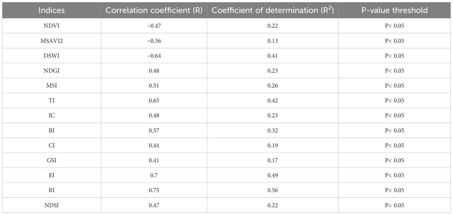
Table 4. Statistical relationships between synthetic image and indices used.

3.2.2 Principal component analysis

One of the key visualizations used to interpret the results of Principal Component Analysis (PCA) is the correlation circle (Figure 6), which offers a two-dimensional graphical representation of the original variables, typically projected onto the first factorial plane. In this diagram, each variable is depicted as a vector, and the direction and length of these vectors indicate how strongly and in what manner each variable contributes to the construction of the principal components. The closer a vector lies to the circle’s perimeter, the better the variable is represented in this plane. Additionally, the squared cosine (cos²) values are employed to quantify the quality of representation of each variable on the principal axes; higher cos² values indicate that a variable is well represented and contributes significantly to the dimension being analyzed in the PCA.

Figure 6

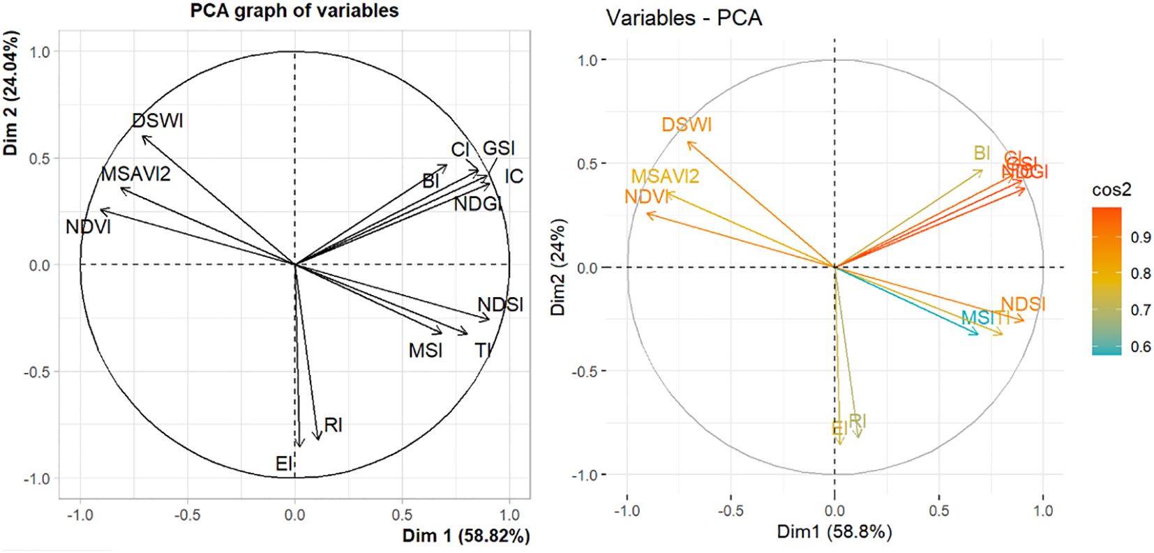
Figure 6. Correlation circles.

The PCA correlation circle can be interpreted as follows:

Vector direction: The direction of the vector indicates the relationship between the original variable and the principal components. The variables NDVI, MSAVI2 and dswi have vectors pointing in the same direction also for the indices NDSI, MSI and texture, which means they are positively correlated and have a similar influence on the principal components (Dim 1). And the vectors of the NDVI, MSAVI2 and dswi indices with the ndsi, msi and texture indices point in opposite directions, meaning they are negatively correlated.

Vector length: The length of the vector indicates the variable’s contribution to the construction of the principal components. The greater the vector length of indices such as color, gsi, ndgi, cuirass, dswi and ndvi, the greater the contribution of the variables to the corresponding axis. Variables with long vectors are considered important in the data structure.

Distance between variables: The distance between vectors of variables indicates their similarity or correlation. The indices color, gsi, ndgi, cuirass is close to each other, are positively correlated and have a similar influence on the principal components. Variables that are far apart, such as redness, texture and ndvi indices, are less correlated and have different influences on the principal components.

This technique extracts the factorial coordinates used in the equation adopted for the model (Table 5). These coordinates were used to project the spectral indices onto the factorial plane defined by the first two principal components. This positioning facilitated the visualization of relationships between indices, the identification of those sharing similar information, and the detection of those indices most representative of the variance observed in the data. Thus, factorial coordinates played an essential role in simplifying and interpreting the structure of spectral indices, guiding the choice of the most relevant variables for modeling water erosion risk.

Table 5

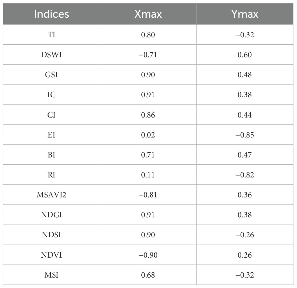
Table 5. Factorial coordinates.

The principal components (PCs) of a data set are linear combinations of variables that capture the maximum variance of the set, by representing proximity vectors adapted to the n observations in a p-dimensional space, while respecting the orthogonality condition between them. PCA is a mathematical method for transforming a set of (possibly correlated) variables into a reduced number of uncorrelated variables, known as PCs. The aim of PCA is to reduce the dimensionality of parameters while highlighting new significant variables. The PCs depend on the units of measurement of the original variables and the range of their values. The first principal component explains as much of the variability in the data as possible, while each subsequent component captures as much of the residual variability as possible (34).

3.3 Final soil degradation map

Modelling produces a cartographic representation of soil exposure to various agents and degradation factors. The table (Table 6) classifies the degree of exposure into five levels, from “lower” to “higher”. The variety of land use types of influences soil composition and condition, which justifies the diversity of the map and the need to use a considerable number of classes to cover all levels of exposure risk.

Table 6

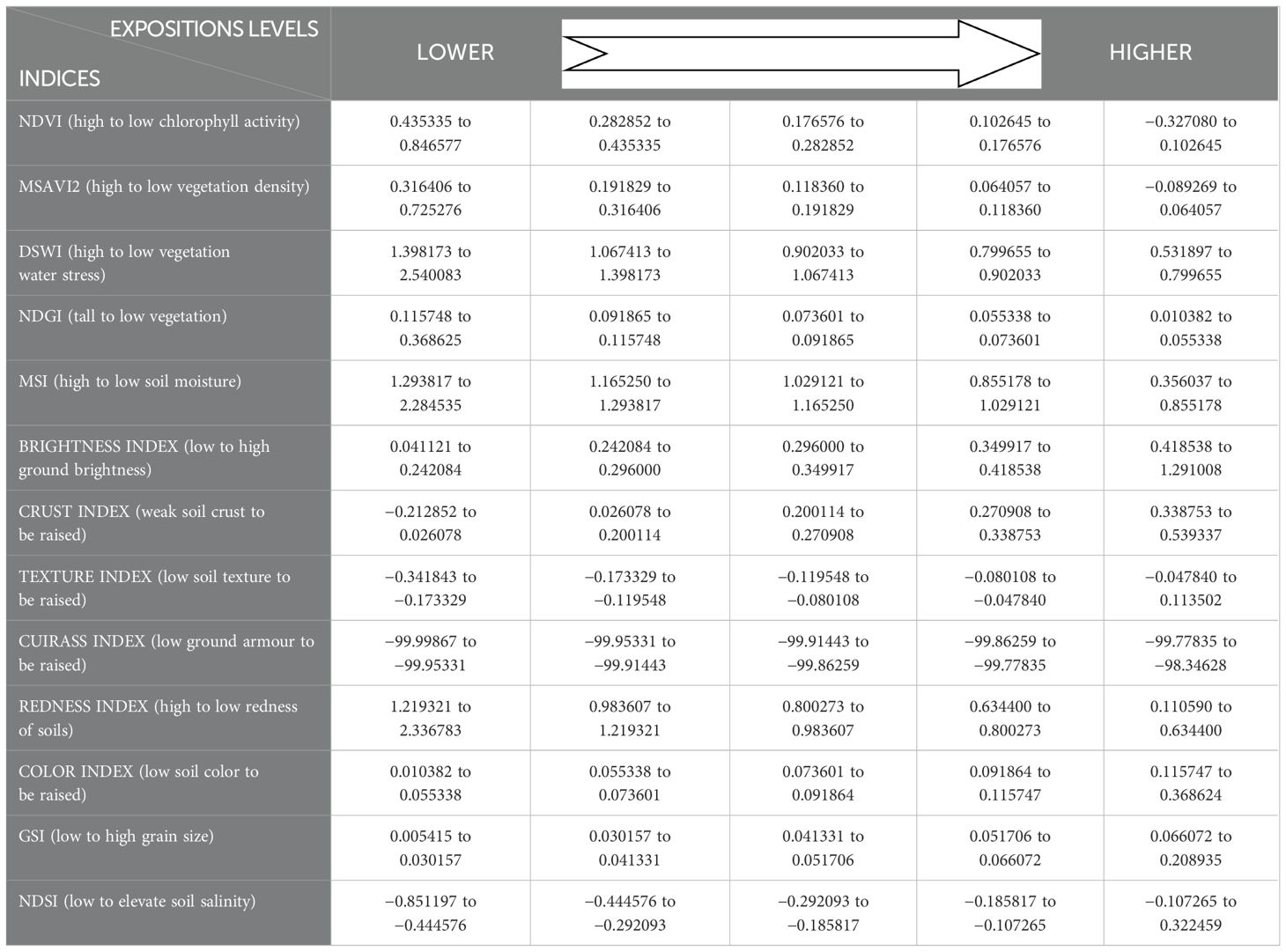
Table 6. Classification of soil degradation levels.

On the combined basis of PCA and linear regression, the indices were grouped into four thematic clusters, each reflecting a specific component of land degradation. For each group, a single index was selected to avoid redundancy while maximizing the representativeness of the information. This selection was based both on the factor contribution in the PCA (coordinates on the principal axes), and on the results of the linear regression, namely the correlation coefficient (R) and the R². The R coefficient indicates the strength and direction of the relationship between the index and erosion risk, while R² reflects the proportion of variability explained by the index. The first group, relating to vegetation moisture and water stress, is represented by the DSWI index, which shows a strong negative correlation (R = −0.64) with erosion and an R² of 0.41, testifying to its explanatory capacity. The second group, relating to surface reflectance and gloss, is represented by the BI index, with an R of 0.57 and an R² of 0.32, showing a good relationship with surface condition and susceptibility to erosion. The third group, focused on soil physical properties (such as texture), is represented by the TI index, which displays a high R (0.65) and an R² of 0.42, positioning it as an important factor in detecting areas at risk. Finally, the fourth group, linked to the chemical or structural characteristics of the soil, is illustrated by the RI index, which stands out with the strongest correlation (R = 0.75) and an R² of 0.56, underlining its predominant role in explaining erosion.

These four indices (DSWI, BI, TI and RI), chosen for their high R and R² values and their significant positioning in the PCA, optimally represent the variability of surface conditions affecting the risk of water erosion, while ensuring a robust simplification of the model.

The approach adopted is to weight the index maps by their coefficient of determination and factor coordinates, to highlight the individual contribution of each index to the final land degradation map. This simplification leads to the following equation:

RISK OF SOIL DEGRADATION = DSWI (Xmax + Ymax) R² + BI (Xmax + Ymax) R² + TI (Xmax + Ymax) R² + RI (Xmax + Ymax) R², ensuring clear, precise and redundancy-free analysis.

RISK OF SOIL DEGRADATION = DSWI * (−0.71 + 0.60) * 0.41 + BI* (0.71 + (0.47)) * 0.32 + TI * (0.80 + (−0.32)) * 0.42 + RI * (0.11 + (−0.82)) * 0.56

After calculating this equation, we obtain a map of the risks of soil exposure to degradation, which is then reclassified to obtain the final map (Figure 7).

Figure 7

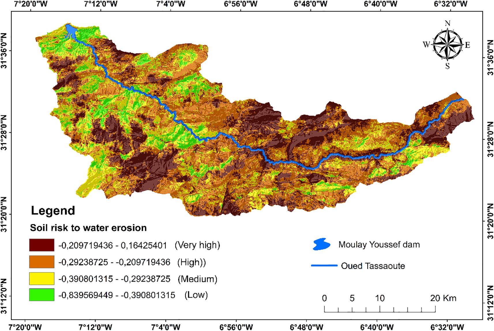
Figure 7. Final soil degradation map.

The spatial distribution of water erosion risk in the upstream Tassaoute watershed reveals a high correlation between soil vulnerability, vegetation cover and local soil properties. Low-risk zones, shown in green, generally coincide with areas of dense vegetation, where roots effectively stabilize the soil, promote water infiltration and reduce runoff. These areas feature well-structured soils, rich in organic matter and with good water retention capacity, limiting susceptibility to erosion. On the other hand, very high-risk areas, shown in brown, are often located on steep, sparsely vegetated slopes, with fragile soils featuring low cohesion, unstable structure, low organic matter content and reduced permeability. This dynamic underscore the importance of sustainable soil and vegetation cover management, incorporating actions such as reforestation, organic amendments and the application of anti-erosion techniques, to curb land degradation and preserve ecosystem functionality in this sensitive region. This need is illustrated in Figure 8, which shows the distribution of surfaces according to their degree of vulnerability to water erosion. It shows that 41.2% of land is classified as high-risk, followed by 27.4% as very high-risk, representing almost 70% of the territory exposed to a critical situation. Conversely, only 8.3% of the area is classified as low risk, underscoring the urgent need for targeted action to reverse this alarming trend.

Figure 8

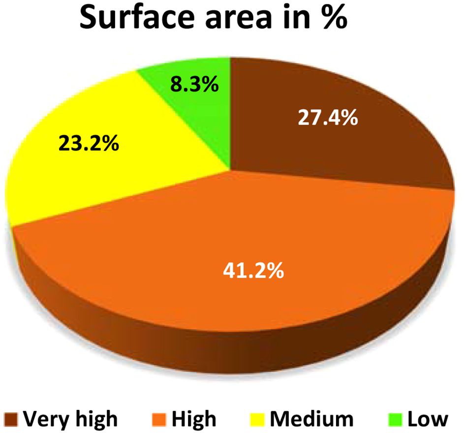
Figure 8. Surface area of degradation levels in %.

4 Validation of results

To assess the performance of the water erosion risk classification model, two complementary approaches were used: the ROC (Receiver Operating Characteristic) curve and the confusion matrix. Although these two tools have different objectives, they are closely linked. The ROC curve is used to analyze the overall ability of the model to distinguish between different classes, independently of a fixed decision threshold. It measures the evolution of the true-positive rate (sensitivity) as a function of the false-positive rate at different thresholds, and the area under the curve (AUC) provides an overall performance indicator. At the same time, the confusion matrix offers a detailed analysis of predictions at a given threshold, precisely identifying good and bad classifications for each class.

On the basis of a field visit to the watershed, field photographs have been taken to validate the results of water erosion risk modelling. They show different types of erosion observed in the field, including gully erosion, badlands, bare slopes and areas of variable vegetation cover. These observations confirm the risk levels identified by the spatial analysis: highly degraded areas correspond to high erosion sectors, while areas with dense vegetation appear less exposed (Figure 9). Several observation points were taken in accessible areas to characterize erosion risk levels (low, medium, high, very high). For hard-to-reach areas, additional points were extracted using the GEE platform, based on visual and topographical criteria and local knowledge. By combining these field points and GEE with spectral indices derived from Sentinel 2A satellite images, a representative dataset was built up.

Figure 9

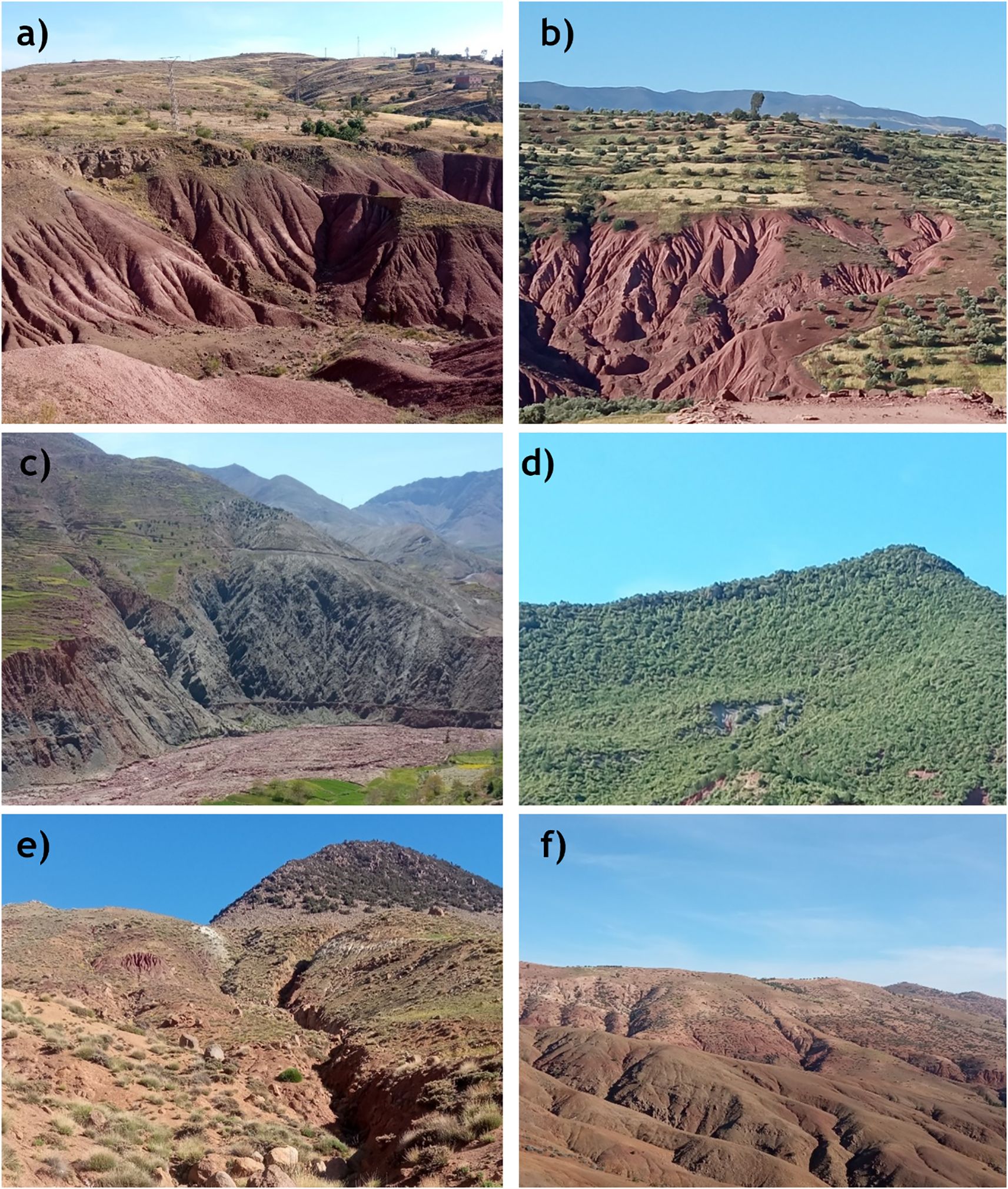
Figure 9. Field illustrations of water erosion forms in the upper Tassaoute watershed. (a) Deep gullying on clay soil; (b) Erosion on terraced cultivated slopes; (c) Marked degradation on steep slopes; (d) Well-vegetated slope at low risk of erosion; (e) Gully formation on bare slopes; (f) Diffuse erosion on arid slopes.

The dataset was then used to train a classification model (Random Forest), and a ROC analysis in One-vs-Rest mode was performed to assess the model’s performance in discriminating each erosion risk class from the others (Figure 10).

Figure 10

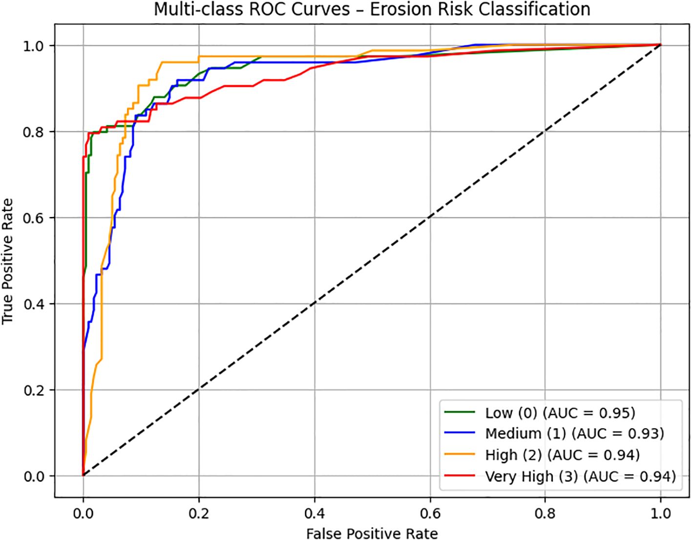
Figure 10. Validation of results by multiclass ROC (in One-vs-Rest mode).

The ROC curve is used to determine model performance, by calculating the area under the curve (AUC). The generalizability of each model was then tested on an external validation cohort. In addition to assessing the discriminating power between each group and the reference group (“one-vs-rest”), it is also essential to evaluate the overall performance of the model in a multi-class classification framework (54).

The multi-class ROC curve obtained shows excellent overall performance. The AUC (Area Under Curve) reaches 0.95 for the “Low” class, 0.93 for “Medium”, 0.94 for “High” and 0.94 for “Very High”. This means that the model can distinguish very effectively the areas corresponding to each level of risk. An AUC close to 1 indicates that the model gives higher probability scores to the true positive classes than to the others, confirming the model’s good discriminatory ability. These results suggest that the spectral index combinations used are relevant for detecting areas at risk of erosion, and that the model can be considered reliable for operational application in this basin.

The confusion matrix (Figure 11) supports the ROC analysis by explicitly showing how the model has classified each observation, i.e. determining the quality of the classification estimated using confusion matrices (55).

Figure 11

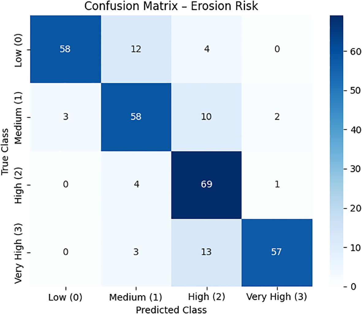
Figure 11. Confusion matrix for the model applied to water erosion risk classification.

In addition, the confusion matrix confirms the model’s accuracy, showing that most samples are correctly classified. For example, 58 samples in the “Weak” class were correctly predicted, compared with only 16 misclassified samples. Similar trends were observed for the other classes: 58 “Medium”, 69 “high” and 57 “Very high” samples were correctly predicted. Errors are mainly concentrated between adjacent classes (e.g. confusion between “Medium” and “High”), which is expected in a continuous phenomenon like erosion. This robustness demonstrates the model’s ability to accurately capture the spatial dynamics of erosion risk, based on both field and satellite data.

5 Discussions

5.1 The influence of vegetation on water erosion

Joint analysis of the soil erosion risk map and vegetation cover data reveals significant relationships between vegetation density and vulnerability to water erosion in our study catchment, with effective management of water resources, notably via Oued Tassaoute and Moulay Youssef dam, crucial to improving water availability and reducing erosion risk (56). A visual comparison of the effectiveness of the vegetation index in discriminating and quantifying canopy density reveals better accuracy when using MSAVI2. Unlike NDVI, MSAVI2 distinguishes more clearly between bare ground and green areas, particularly in less forested regions. In addition, this index assigns low values to aquatic areas, unlike the DSWI and NDGI indices. These findings are in line with previous results demonstrating the effectiveness of MSAVI2 for vegetation mapping in arid environments (27).

The results obtained in this study confirm and are in line with the abundant scientific literature highlighting the central role of vegetation cover in regulating water erosion. Numerous studies, notably those by (57), have demonstrated that the density, type and spatial distribution of vegetation significantly influence the reduction of runoff and soil loss. Rey notes that water erosion tends to decrease as vegetation cover increases, with vegetated surfaces offering better protection against the detachment and transport of soil particles, in contrast to bare areas, which are particularly vulnerable, especially on slopes. Other authors, such as (58, 59), highlight the influence of climatic conditions on plant growth, and therefore on the ability of the cover to buffer the erosivity of rainfall. In this sense, vegetation acts as a physical barrier that absorbs raindrop energy, reduces direct impact on the soil, and limits particle splash. These authors also stress the importance of seasonal variations and vegetation types, as well as the role of agricultural practices in the dynamics of vegetation cover. And recent literature complements these observations with more mechanistic analyses: (60) highlights the correlation between root density and soil stability, while (61) shows that organic litter contributes significantly to reducing soil losses in agroforestry systems, accounting for up to 90% of erosion variability. Simple arrangements such as grass strips, when judiciously placed, can also effectively reduce runoff and sediment (62, 63). The functional diversity of plant species, in particular their height, leaf system and root system, also appears to play a crucial role in the overall effectiveness of erosion control (64). Finally, (65) points out that the mechanical resistance provided by vegetation can account for up to 50% of overall erosion resistance, underlining the importance of dense, structured and diversified plant cover in preserving soil and water resources.

In short, these results confirm that vegetation cover, in both its quantitative (density) and qualitative (diversity, structure) aspects, is a major lever for the sustainable management of water erosion. The mapping of spectral indices used in this study enables a fine spatialization of these dynamics, providing valuable operational support for watershed management and conservation.

5.2 The influence of soil on water erosion

Cross-analysis of the erosion risk map and soil property indices reveals significant relationships between soil characteristics and vulnerability to water erosion in the watershed studied. Factors such as texture, crust, color and chemical properties directly influence soil structural stability in the face of water action. Fine texture, often composed of clays, limits water infiltration, thus favoring surface runoff (23, 58, 66). However, this texture is not necessarily more sensitive to stripping than the medium texture, a nuance provided by several authors (23, 66). On the other hand, sandy soils, although highly permeable, have low cohesion, making them susceptible to detachment under the impact of raindrops (67). Organic matter plays an essential role in erosion resistance. It improves soil structure, increases porosity and acts as a binder between mineral particles, promoting aggregation (68–70). This stabilizing role has been confirmed in several studies of Mediterranean watersheds (71, 72), where surface horizons poor in organic matter and fine-textured prove particularly vulnerable to erosion. The results of this study are consistent with those reported in other geographical contexts, notably in Lebanon, where CNRSL researchers (69, 73) have highlighted the major influence of soil structure – dependent on texture and organic matter – on susceptibility to water erosion. In addition, spectral indices linked to soil color, such as intensity, hue or saturation, can be used to detect levels of degradation (24), providing a promising tool for erosion mapping and prevention.

In short, soil stability against water erosion depends on a combination of physical and organic properties, including texture, structure, porosity and organic matter. These parameters must be taken into account in any approach to sustainable soil management.

6 Conclusion

Among the most severe levels of degradation, the “high” level is the most widespread, covering 583.13 km², followed by the “very high” level with 387.66 km², the “medium” level, which covers 329.56 km², and finally the “weak” level, which covers 117.99 km².

This research has demonstrated the importance and contribution of remote sensing to the mapping of areas at risk of water erosion. The application of the spectral index method, using remote sensing and spatial analysis techniques, based on spectral indices (vegetation indices, soil indices) will enable us to estimate, understand and analyze the problem of erosion risk in the study area. This method has proven its effectiveness and speed in providing a general diagnosis of the risk of water erosion at the scale of the upstream Tassaoute watershed.

The objective was to model the risk of soil degradation in the upstream Tassaoute watershed by combining spectral indices with statistical analysis. The results were strongly correlated with factors such as the phenological season during which the satellite images were acquired, the quality of the images, the formula of the indices used, and the statistical treatments applied. A statistical analysis was then performed on the resulting image, providing, on one hand, the correlation and determination coefficients of each index, and on the other hand, the factorial axes that summarize more information. All indices are considered statistically significant (P value < 0.05).

However, our methodology is currently applied to images from specific months in 2021 (August and September). The challenge now is to adapt the model to data from previous years and different times of the year. Additionally, the exclusion of urban areas presents a limitation, as elements typical of built environments (e.g., aluminum roofing) inevitably influence the calculation of certain indices.

The disparity between the number of vegetation indices and soil indices must be addressed through a readjustment that will enable the integration of additional parameters, such as surface temperature, precipitation, albedo, and evapotranspiration. Other factors, including topography and the distribution of the hydrographic network, should also be considered.

Given the imminent threat of deterioration of natural resources such as forests, water, soil and biodiversity, as well as the economic and social consequences for the quality of life of residents, it has become urgent to take action to combat erosion. This intervention adopts a global and innovative approach, which seeks to reconcile the growing needs of the population, faced with continuous growth, with the increasingly depleted limited natural resources, also considering the impact of climate change.

To deepen our understanding of soil degradation, it would be beneficial to integrate other techniques such as geochemical data to assess soil degradation. Geochemistry studies the chemical composition of terrestrial materials, including soils. Moreover, the use of isotopic techniques can provide additional information on soil degradation processes. The integration of geochemical data, by combining chemical and isotopic analyses, as well as the use of portable or field technologies, opens new perspectives for assessing soil degradation.

Finally, several methodological limitations need to be highlighted. Dependence on satellite data can introduce biases related to cloud cover or spatial resolution. The temporal selection of images limits seasonal representativeness, and ground sampling remains spatially restricted. Furthermore, although performance has been validated by robust indicators (ROC, confusion matrix), generalization of the model to other geographical contexts requires specific adjustments. These limitations open prospects for future research integrating more in situ data, complementary sensors and temporally dynamic models.

Data availability statement

The raw data supporting the conclusions of this article will be made available by the authors, without undue reservation.

Author contributions

ON-T: Conceptualization, Formal analysis, Software, Writing – original draft, Writing – review & editing. SE: Investigation, Methodology, Visualization, Writing – original draft. KA: Funding acquisition, Investigation, Resources, Visualization, Writing – review & editing. MI: Conceptualization, Formal analysis, Methodology, Software, Validation, Visualization, Writing – review & editing. MF: Formal analysis, Funding acquisition, Visualization, Writing – review & editing. JA: Methodology, Software, Writing – review & editing. IO: Investigation, Visualization, Writing – review & editing. IK: Data curation, Validation, Visualization, Writing – review & editing. SK: Conceptualization, Software, Visualization, Writing – review & editing. MN: Formal analysis, Methodology, Software, Visualization, Writing – review & editing. AE: Conceptualization, Project administration, Software, Supervision, Validation, Visualization, Writing – review & editing.

Funding

The author(s) declare that financial support for the research and/or publication of this article was received from the Ongoing Research Funding Program (ORF-2025-249), King Saud University, Riyadh, Saudi Arabia.

Acknowledgments

The authors extend their sincere appreciation to the Ongoing Research Funding Program (ORF-2025-249), King Saud University, Riyadh, Saudi Arabia, for funding this research. They also gratefully acknowledge the support of the PRIMA Resilink and GEANTech projects for their invaluable contribution to this research article. Special thanks are extended to the anonymous reviewers for their insightful and constructive comments.

Conflict of interest

The authors declare that the research was conducted in the absence of any commercial or financial relationships that could be construed as a potential conflict of interest.

Generative AI statement

The author(s) declare that Generative AI was used in the creation of this manuscript. During the preparation of this work, the authors utilized GPT-4 to correct the grammar and structure of the English language, ensuring clarity in the sentences for the reader. After using this tool/service, the author reviewed and edited the content as needed and took full responsibility for the publication’s content.

Publisher’s note

All claims expressed in this article are solely those of the authors and do not necessarily represent those of their affiliated organizations, or those of the publisher, the editors and the reviewers. Any product that may be evaluated in this article, or claim that may be made by its manufacturer, is not guaranteed or endorsed by the publisher.

References

1. Mosaid H, Barakat A, Bustillo V, and Rais J. Modeling and mapping of soil water erosion risks in the Srou Basin (Middle Atlas, Morocco) using the EPM model, GIS and magnetic susceptibility. J Landscape Ecol. (2022) 15:126–47. doi: 10.2478/jlecol-2022-0007

Crossref Full Text | Google Scholar

2. ENNASSIRI B. Modélisation du risque d’érosion des sols dans le bassin versant de N’Fis Utilisation de l’Equation Universelle Révisée des Pertes en Sols (RUSLE). In: Revue Marocaine de Géomorphologie. Badreddine Ennassiri: University of Hassan II Casablanca (2021). Available at: https://revues.imist.ma/index.php/Remageom/article/view/25621.

Google Scholar

3. Aboutaib F, Krimissa S, Pradhan B, Elaloui A, Ismaili M, Abdelrahman K, et al. Evaluating the effectiveness and robustness of machine learning models with varied geo-environmental factors for determining vulnerability to water flow-induced gully erosion. Front Environ Sci. (2023) 11:1207027. doi: 10.3389/fenvs.2023.1207027

Crossref Full Text | Google Scholar

4. Borrelli P, Alewell C, Alvarez P, Anache JAA, Baartman J, Ballabio C, et al. Soil erosion modelling: A global review and statistical analysis. Sci Total Environ. (2021) 780:146494. doi: 10.1016/j.scitotenv.2021.146494

PubMed Abstract | Crossref Full Text | Google Scholar

5. Eloudi H, Hssaisoune M, Reddad H, Namous M, Ismaili M, Krimissa S, et al. Robustness of optimized decision tree-based machine learning models to map gully erosion vulnerability. Soil Syst. (2023) 7:50. doi: 10.3390/soilsystems7020050

Crossref Full Text | Google Scholar

6. Borrelli P, Poesen J, Vanmaercke M, Ballabio C, Hervás J, Maerker M, et al. Monitoring gully erosion in the European Union: A novel approach based on the Land Use/Cover Area frame survey (LUCAS). Int Soil Water Conserv Res. (2022) 10:17–28. doi: 10.1016/j.iswcr.2021.09.002

Crossref Full Text | Google Scholar

7. Tien Bui D, Shirzadi A, Shahabi H, Chapi K, Omidavr E, Pham BT, et al. A novel ensemble artificial intelligence approach for gully erosion mapping in a semi-arid watershed (Iran). Sensors. (2019) 19:2444. doi: 10.3390/s19112444

PubMed Abstract | Crossref Full Text | Google Scholar

8. Gómez-Gutiérrez Á, Conoscenti C, Angileri SE, Rotigliano E, and Schnabel S. Using topographical attributes to evaluate gully erosion proneness (susceptibility) in two mediterranean basins: advantages and limitations. Nat Hazards. (2015) 79:291–314. doi: 10.1007/s11069-015-1703-0

Crossref Full Text | Google Scholar

9. Arabameri A, Pradhan B, and Rezaei K. Gully erosion zonation mapping using integrated geographically weighted regression with certainty factor and random forest models in GIS. J Environ Manage. (2019) 232:928–42. doi: 10.1016/j.jenvman.2018.11.110

PubMed Abstract | Crossref Full Text | Google Scholar

10. Acharki S, El Qorchi F, Arjdal Y, Amharref M, Bernoussi AS, and Aissa HB. Soil erosion assessment in Northwestern Morocco. Remote Sens Applications: Soc Environ. (2022) 25:100663. doi: 10.1016/j.rsase.2021.100663

Crossref Full Text | Google Scholar

11. El Amarty F, Lahrach A, Benaabidate L, and Chakir A. Estimating soil erosion and sediment yield using GIS in the central pre-rif (Northern Morocco)–the case of the oued lebene watershed. In: Ecological engineering & Environmental technology (EEET) FST-Fés, Sidi Mohammed BenUniversitè Abdellah, Route d'Immouzer, BP : 2202, Fez 30000, Maroc, vol. 25. (2024). Available at: https://www.researchgate.net/profile/Fahed-El-Amarty-2/publication/381604714_Estimating_Soil_Erosion_and_Sediment_Yield_Using_Geographic_Information_System_in_the_Central_Pre-Rif_Northern_Morocco_-_The_Case_of_the_Oued_Lebene_Watershed/links/66759822d21e220d89c59f5a/Estimating-Soil-Erosion-and-Sediment-Yield-Using-Geographic-Information-System-in-the-Central-Pre-Rif-Northern-Morocco-The-Case-of-the-Oued-Lebene-Watershed.pdf.

Google Scholar

12. Elaloui A, Marrakchi C, Fekri A, Maimouni S, and Aradi M. Mise en place d’un modèle qualitatif pour la cartographie des zones à risque d’érosion hydrique dans la chaîne atlasique: cas du bassin versant de la tessaoute amont.(haut atlas central, maroc). Eur Sci J. (2015) 11, 29. hal-00681436

Google Scholar

13. Elaloui A, Marrakchi C, Fekri A, Maimouni S, and Aradi M. USLE-based assessment of soil erosion by water in the watershed upstream Tessaoute (Central High Atlas, Morocco). Model Earth Syst Environ. (2017) 3:873–85. doi: 10.1007/s40808-017-0340-x

Crossref Full Text | Google Scholar

14. Elaloui A, Khalki EME, Namous M, Ziadi K, Eloudi H, Faouzi E, et al. Soil erosion under future climate change scenarios in a semi-arid region. Water. (2023) 15:146. doi: 10.3390/w15010146

Crossref Full Text | Google Scholar

15. Remini W and Remini B. La sedimentation dans les barrages de L’afrique du nord.

Google Scholar

16. El Jihad M-D. Croissance urbaine et problèmes d’assainissement liquide et pluvial dans le bassin du Srou (Maroc central). Sci changements planétaires/Sécheresse. (2005) 16(1):41–52.

Google Scholar

17. Yammad Y and Baddih H. L’incidence de l’accès à l’eau potable et aux services d’assainissement sur la croissance économique et l’IDH: Cas du Maroc. In: Congrès Interdisciplinaire sur l’Economie Circulaire CIEC-2024. (2024) Montpellier, France. hal-04967042. Available at: https://hal.science/hal-04967042/document.

Google Scholar

18. Ismaili M, Krimissa S, Namous M, Htitiou A, Abdelrahman K, Fnais MS, et al. Assessment of soil suitability using machine learning in arid and semi-arid regions. Agronomy. (2023) 13:165. doi: 10.3390/agronomy13010165

Crossref Full Text | Google Scholar

19. Keay-Bright J and Boardman J. The influence of land management on soil erosion in the Sneeuberg Mountains, Central Karoo, South Africa. Land Degrad Dev. (2007) 18:423–39. doi: 10.1002/ldr.785

Crossref Full Text | Google Scholar

20. Khemiri K and Jebari S. Évaluation de l’érosion hydrique dans des bassins versants de la zone semi-aride tunisienne avec les modèles RUSLE et MUSLE couplés à un Système d’information géographique. Cahiers Agricultures. (2021) 30:7. doi: 10.1051/cagri/2020048

Crossref Full Text | Google Scholar

21. Fadil A and Wahidi FE. Vers une nouvelle classification des modèles d’évaluation et de prédiction de l’érosion hydrique. Physio-Géo Géographie physique environnement. (2023), 83–112. doi: 10.4000/physio-geo.15783

Crossref Full Text | Google Scholar

22. El Jazouli A. cartographie et modélisation des risques d’érosion hydrique et de glissement de terrain au niveau du bassin amont d’oum er rbia (2020). Available online at: https://toubkal.imist.ma/handle/123456789/25586 (Accessed June 1, 2025).

Google Scholar

23. Maimouni S. exploitation des données du capteur advanced land imager et du modèle numérique d’altitude pour la cartographie de l’érosion hydrique dans le pourtour du barrage hassan 1er au maroc (2012). Available online at: https://toubkal.imist.ma/handle/123456789/25656 (Accessed December 14, 2024).

Google Scholar

24. Haboudane D. Intégration des données spectrales et géomorphométriques pour la caractérisation de la dégradation des sols et l’identification des zones de susceptibilité à l’érosion hydrique. Ottawa: National Library of Canada= Bibliothèque nationale du Canada (2002). Available at: https://library-archives.canada.ca/eng/services/services-libraries/theses/Pages/item.aspx?idNumber=53823846.

Google Scholar

25. El Ghachi M. Impact des actions anthropiques sur le bilan hydrologique dans le bassin versant de la Tassaout (amont du barrage Moulay Youssef): modèle hydrologique Orchy II (1986-2010). J Water Environ Sci. (2018) 2:297–304.

Google Scholar

26. Chakir M, Ghadbane O, Ouakhir H, and El G. Extraction et analyse des phases de tarissement: application dans le bassin versant de l’oued Tassaout (amont du Barrage Moulay Youssef), Haut Atlas Central, Maroc (1978-2016). Afrique Sci. (2023) 22:129–41.

Google Scholar

27. Gadal S, Gbetkom P, and Mfondoum A. A new soil degradation method analysis by sentinel 2 images combining spectral indices and statistics analysis: application to the Cameroonians shores of lake Chad and its hinterland. In: Proceedings of the 7th international conference on geographical information systems theory, applications and management. AMU - Aix Marseille Université: SCITEPRESS - Science and Technology Publications (2021). p. 25–36. doi: 10.5220/0010521200250036

Crossref Full Text | Google Scholar

28. Guo M, Yu Z, Xu Y, Huang Y, and Li C. ME-net: A deep convolutional neural network for extracting mangrove using Sentinel-2A data. Remote Sens. (2021) 13:1292. doi: 10.3390/rs13071292

Crossref Full Text | Google Scholar

29. Boiffin J, Papy F, and Eimberck M. Influence des systèmes de culture sur les risques d’érosion par ruissellement concentré. I.–Analyse des conditions de déclenchement de l’érosion. Agronomie. (1988) 8:663–73. doi: 10.1051/agro:19880801

Crossref Full Text | Google Scholar

30. Gallien E, Le Bissonnais Y, Eimberck M, Benkhadra H, Ligneau L, Ouvry J-F, et al. Influence des couverts végétaux de jachère sur le ruissellement et l’érosion diffuse en sol limoneux cultivé. Cahiers Agricultures. (1995) 4:171–83.

Google Scholar

31. Abdou MM. Trends in re-greening and soil degradation in western Niger. Environ Water Sciences Public Health Territorial Intell J. (2019) 3:96–103. doi: 10.48421/IMIST.PRSM/ewash-ti-v3i2.15896

Crossref Full Text | Google Scholar

32. Ismaili M, Krimissa S, Namous M, Abdelrahman K, Boudhar A, Edahbi M, et al. Mapping soil suitability using phenological information derived from MODIS time series data in a semi-arid region: A case study of Khouribga, Morocco. In: Heliyon, vol. 10. (2024). Available at: https://www.cell.com/heliyon/fulltext/S2405-8440(24)00132-4.

PubMed Abstract | Google Scholar

33. Rouse JW, Haas RH, Schell JA, and Deering DW. Monitoring vegetation systems in the Great Plains with ERTS. NASA Spec. Publ. (1974) 351:309.

Google Scholar

34. Sharma KL, Grace JK, Mandal UK, Gajbhiye PN, Srinivas K, Korwar GR, et al. Evaluation of long-term soil management practices using key indicators and soil quality indices in a semi-arid tropical Alfisol. Soil Res. (2008) 46:368–77. doi: 10.1071/SR07184

Crossref Full Text | Google Scholar

35. Söderström M, Piikki K, Stenberg M, Stadig H, and Martinsson J. Producing nitrogen (N) uptake maps in winter wheat by combining proximal crop measurements with Sentinel-2 and DMC satellite images in a decision support system for farmers. Acta Agriculturae Scandinavica Section B — Soil Plant Sci. (2017) 67:637–50. doi: 10.1080/09064710.2017.1324044

Crossref Full Text | Google Scholar

36. Qi J, Chehbouni A, Huete AR, Kerr YH, and Sorooshian S. A modified soil adjusted vegetation index. Remote Sens Environ. (1994) 48:119–26. doi: 10.1016/0034-4257(94)90134-1

Crossref Full Text | Google Scholar

37. Bochenek Z, Dąbrowska-Zielińska K, Gurdak R, Niro F, Bartold M, and Grzybowski P. Validation of the LAI biophysical product derived from Sentinel-2 and Proba-V images for winter wheat in western Poland. Geoinformation Issues. (2017) 9:15–26.

Google Scholar

38. Nedkov R. Normalized differential greenness index for vegetation dynamics assessment. (2017) 70(8):1143–6.

Google Scholar

39. Benabdelouahab T, Balaghi R, Hadria R, Lionboui H, and Tychon B. Assessment of vegetation water content in wheat using near and shortwave infrared SPOT-5 Data in an irrigated area. rseau. (2016) 29:97–107. doi: 10.7202/1036542ar

Crossref Full Text | Google Scholar

40. Li S, Yuan F, Ata-UI-Karim ST, Zheng H, Cheng T, Liu X, et al. Combining color indices and textures of UAV-based digital imagery for rice LAI estimation. Remote Sens. (20191763) 11(15):1763. doi: 10.3390/rs11151763

Crossref Full Text | Google Scholar

41. Maimouni S, Bannari A, El-Harti A, and El-Ghmari A. Potentiels et limites des indices spectraux pour caractériser la dégradation des sols en milieu semi-aride. Can J Remote Sens. (2011) 37:285–301. doi: 10.5589/m11-038

Crossref Full Text | Google Scholar

42. Ramos TB, Castanheira N, Oliveira AR, Paz AM, Darouich H, Simionesei L, et al. Soil salinity assessment using vegetation indices derived from Sentinel-2 multispectral data. application to Lezíria Grande, Portugal. Agric Water Manage. (2020) 241:106387. doi: 10.1016/j.agwat.2020.106387

Crossref Full Text | Google Scholar

43. Okaingni J-C, Kouamé KF, and Martin A. Mapping breastplates in volcano-sedimentary area of anikro-kadiokro (Ivory coast) using the dempster-shafer theory of evidence. Rev Télédétection. (2010) 9:19–32.

Google Scholar

44. Laboratory of Natural Resources Management, Department of Geography, University of Yaoundé I, Cameroon, Ngandam Mfondoum AH, Etouna J, Laboratory of Remote Sensing and Spatial Analysis, National Institute of Cartography, Yaoundé, Cameroon, et al. Assessment of land degradation status and its impact in arid and semi-arid areas by correlating spectral and principal component analysis neo-bands. IJARSG. (2016) 5:1539–60. doi: 10.23953/cloud.ijarsg.77

Crossref Full Text | Google Scholar

45. Ambouta KJ. Etude des facteurs de formation d’une croute d’erosion et de ses relations avec les proprietes internes d’un sol sableux fin au Sahel (1996). Available online at: https://elibrary.ru/item.asp?id=5601796 (Accessed June 1, 2025).

Google Scholar

46. Devineau J-L. Utilisation de l’indice de rougeur de Madeira pour la reconnaissance des sols de la région de Bondoukuy (ouest burkinabé) à partir d’images satellitaires SPOT., in Surveillance des Sols dans l’Environnement par Télédétection et Systèmes d’Information Géographiques: Symposium International AISS (Groupes de Travail RS: Télédétection et Cartographie des Sols et DM: Carte Internationale Numérique des Sols et des Terrains)= Monitoring Soils in the Environment with Remote Sensing and GIS: ISSS International Symposium (Working Groups RS and DM), (Orstom) (1995). Available online at: https://ird.hal.science/ird-00357128/ (Accessed June 1, 2025).

Google Scholar

47. Nguyen CT, Chidthaisong A, Kieu Diem P, and Huo L-Z. A modified bare soil index to identify bare land features during agricultural fallow-period in southeast Asia using Landsat 8. Land. (2021) 10:231. doi: 10.3390/land10030231

Crossref Full Text | Google Scholar

48. Uyanık GK and Güler N. A study on multiple linear regression analysis. Proc - Soc Behav Sci. (2013) 106:234–40. doi: 10.1016/j.sbspro.2013.12.027

Crossref Full Text | Google Scholar

49. Foucart T. Colinéarité et régression linéaire. In: Mathématiques et sciences humaines. Mathematics and social sciences (2006). doi: 10.4000/msh.2963

Crossref Full Text | Google Scholar

50. Mfondoum AHN, Etouna J, Nongsi BK, Moto FM, and Deussieu FN. Assessment of land degradation status and its impact in arid and semi-arid areas by correlating spectral and principal component analysis neo-bands. Int J Advanced Remote Sens GIS. (2016) 5:1539–60. doi: 10.23953/cloud.ijarsg.77

Crossref Full Text | Google Scholar

51. Mouissi S and Alayat H. Utilisation de l’Analyse en Composantes Principales (ACP) pour la caractérisation Physico-chimique des eaux d’un écosystème aquatique: Cas du Lac Oubéira (Extrême NE Algérien). J Materials Environ Sci. (2016) 7:2214–20.

Google Scholar

52. Aied M. ETUDE QSAR DE CERTAIN DERIVES 7-SUBSTUTUÉ 4-AMINOQUINOLINE COMME DES AGENTS ANTIPALUDIQUE. 2018 (2018). Available online at: http://archives.univ-biskra.dz/handle/123456789/12026 (Accessed May 7, 2025).

Google Scholar

53. Guerrien M. L’intérêt de l’analyse en composantes principales (ACP) pour la recherche en sciences sociales. Présentation à partir d’une étude sur le Mexique. Cahiers Des Amériques latines. (2003), 181–92. doi: 10.4000/cal.7364

Crossref Full Text | Google Scholar

54. Chen Z, Xu L, Zhang C, Huang C, Wang M, Feng Z, et al. CT radiomics model for discriminating the risk stratification of gastrointestinal stromal tumors: a multi-class classification and multi-center study. Front Oncol. (2021) 11:654114. doi: 10.3389/fonc.2021.654114

PubMed Abstract | Crossref Full Text | Google Scholar

55. Sparfel L, Gourmelon F, and Le Berre I. Approche orientée-objet de l’occupation des sols en zone côtière. Télédétection. (2010) 8(4):237–56.

Google Scholar

56. Baiddah A, Krimissa S, Hajji S, Ismaili M, Abdelrahman K, El Bouzekraoui M, et al. Head-cut gully erosion susceptibility mapping in semi-arid region using machine learning methods: insight from the high atlas, Morocco. Front Earth Sci. (2023) 11:1184038. doi: 10.3389/feart.2023.1184038

Crossref Full Text | Google Scholar

57. Rey F, Ballais J-L, Marre A, and Rovéra G. Rôle de la végétation dans la protection contre l’érosion hydrique de surface. Comptes rendus. Géoscience. (2004) 336:991–8. doi: 10.1016/j.crte.2004.03.012

Crossref Full Text | Google Scholar

58. Hassan HEH, Touchart L, and Faour G. La sensibilité potentielle du sol à l’érosion hydrique dans l’ouest de la Bekaa au Liban. In: M@ ppemonde. (2013). Université d’Orléans, Laboratoire CEDETE (EA 1210) Centre national de télédétection, Liban. Available at: https://hal.science/hal-01962928/.

Google Scholar

59. Ousmana H, El Hmaidi A, Essahlaoui A, Bekri H, and El Ouali A. Modélisation et cartographie du risque de l’érosion hydrique par l’application des SIG et des directives PAP/CAR. Cas du bassin versant de l’Oued Zgane (Moyen Atlas tabulaire, Maroc). Bull l’Institut Scientifique Rabat Section Sci la Terre. (2017) 39:103–19.

Google Scholar

60. Dahanayake AC, Webb JA, Greet J, and Brookes JD. How do plants reduce erosion? An Eco Evidence assessment. Plant Ecol. (2024) 225:593–604. doi: 10.1007/s11258-024-01414-9

Crossref Full Text | Google Scholar

61. Blanco-Sepúlveda R, Lima F, and Aguilar-Carrillo A. An assessment of the shade and ground cover influence on the mitigation of water-driven soil erosion in a coffee agroforestry system. Agroforest Syst. (2024) 98:1771–82. doi: 10.1007/s10457-024-00989-6

Crossref Full Text | Google Scholar

62. Zhang X, Li P, Bin Li Z, and Qiang Yu G. Effects of grass strips distribution on soil erosion and its optimal configuration on hillslopes. CATENA. (2024) 238:107882. doi: 10.1016/j.catena.2024.107882

Crossref Full Text | Google Scholar

63. Zhou S, Li P, Zhang X, Wang Y, Yu K, Shi P, et al. Runoff and erosion reduction benefits of vegetation during natural succession on fallow grassland slopes. Sci Total Environ. (2024) 954:176211. doi: 10.1016/j.scitotenv.2024.176211

PubMed Abstract | Crossref Full Text | Google Scholar

64. Seitz S, Gall C, Riveras-Muñoz Nicolás, Song Z, and Scholten T. Étude des effets de différentes couches de végétation sur l'érosion des sols à l'aide d'un simulateur de précipitations portable. Dans: EGU General Assembly Conference Abstracts. (2024). p. 3431.

Google Scholar

65. Liu C, Zhang K, Wei S, Wang P, Cen Y, and Xia J. Evaluation of the effects of grass and shrub cover on overland flow resistance and its attributes under simulated rainfall. J Hydrology. (2023) 626:130285. doi: 10.1016/j.jhydrol.2023.130285

Crossref Full Text | Google Scholar

66. Roose E, Arabi M, Brahamia K, Chebbani R, Mazour M, and Morsli B. Érosion en nappe et ruissellement en montagne méditerranéenne algérienne. Cahiers Orstom série pédologie. (1993) 28:289–308.

Google Scholar

67. Morgan RPC and Hann MJ. Design of diverter berms for soil erosion control and biorestoration along pipeline rights-of-way. Soil Use Manage. (2005) 21:306–11. doi: 10.1111/j.1475-2743.2005.tb00403.x

Crossref Full Text | Google Scholar

68. Duchaufour P. Précis de pédologie (1970). Available online at: https://www.sidalc.net/search/Record/KOHA-OAI-AGRO:6594/Description (Accessed June 2, 2025).

Google Scholar

69. Kheir RB, Girard M-C, Shaban A, Khawlie M, FAOUR G, and Darwich T. Apport de la télédétection pour la modélisation de l’érosion hydrique des sols dans la région côtière du Liban. Télédétection. (2001) 2:79–90.

Google Scholar

70. Mohsine Y. Application du magnétisme de l’environnement pour la caractérisation de l’état d’évolution et/ou de dégradation des sols: Application aux sous bassins versants de Mezguida et Ait Azzouz de Bouregreg (2009). Available online at: https://toubkal.imist.ma/handle/123456789/12975 (Accessed December 14, 2024).

Google Scholar

71. Lal R. Soil degradation by erosion. Land Degrad Dev. (2001) 12:519–39. doi: 10.1002/ldr.472

Crossref Full Text | Google Scholar

72. El Bouzekraoui M, Elaloui A, Krimissa S, Abdelrahman K, Kahal AY, Hajji S, et al. Performance assessment of individual and ensemble learning models for gully erosion susceptibility mapping in a mountainous and semi-arid region. Land. (2024) 13:2110. doi: 10.3390/land13122110

Crossref Full Text | Google Scholar

73. Darwish TM and Zurayk RA. Distribution and nature of Red Mediterranean soils in Lebanon along an altitudinal sequence. Catena. (1997) 28:191–202. doi: 10.1016/S0341-8162(96)00037-9

Crossref Full Text | Google Scholar