Spatiotemporal prediction of soil moisture content at various depths in three soil types using machine learning algorithms

Introduction: Accurate prediction of soil moisture content (SMC) is crucial for agricultural systems as it affects hydrological cycles, crop growth, and resource management. Considering the challenges with prediction accuracy and determining the effect of soil texture, depth, and meteorological data on SMC variation and prediction capability of the used models, this research has been conducted.

Methods: Three machine learning (ML) models—random forest regression (RFR), eXtreme gradient boosting (XGBoost), and long short-term memory (LSTM)—were developed to predict SMC in three soil types (loam, sandy loam, and silt loam) at five depths of 5, 20, 40, 60, and 80 cm. The dataset was collected during the maize season in 2023, encompassing meteorological parameters collected using Internet of Things (IoT)-based sensors and SMC data calculated using the gravimetric method.

Results: The results showed variations in SMC in all studied soil types and depths, with silt loam exhibiting the highest variation in SMC. RFR demonstrated high accuracy at different depths and soil types, particularly in loam soil, at a depth of 80 with a root mean square error (RMSE) value of 0.89 and a mean absolute error (MAE) value of 0.74, and in silt loam at 40 cm depth with an RMSE value of 0.498 and an MAE of 0.416. LSTM performed effectively at shallower and moderate depths (60 and 20 cm) with RMSE values of 0.391 and 0.804 and MAE values of 0.335 and 0.793, respectively. In sandy loam soil at 5 cm depth, XGBoost displayed minimal errors and robust performance at the same depths with higher accuracy, achieving an RMSE of 0.025 and an MAE of 0.159. Analysis of training and validation loss revealed that the LSTM model stabilized and improved with more epochs, showing a more consistent decrease in MSE, while RFR and XGBoost exhibited higher performance with increased model complexity, shown in low MSE and RMSE values. Comparisons between measured and predicted SMC% values demonstrated the models’ effectiveness in capturing soil moisture dynamics. Furthermore, feature importance analysis revealed that solar radiation and precipitation were the most influential predictors across all models, offering critical insights into dominant environmental drivers of soil moisture variability.

Discussion: By providing precise SMC predictions across different spatial and temporal scales, this study underscores the value of ML models for SMC prediction, which could have implications for improving irrigation scheduling, reducing water wastages, and enhancing sustainability.

1 Introduction

Current farming practices have already exceeded the Earth’s carrying capacity (1). Therefore, the primary challenge is to enhance productivity and sustainably feed the world without depleting natural resources, particularly water, which is vital for crop production. Hence, it is imperative to implement more sustainable water management practices (2). With the increased demand for agricultural water resources, real-time monitoring of soil moisture is essential for developing a realistic irrigation schedule, leading to better water management (3, 4), and enhancing crop production (5). Soil moisture content (SMC) is a critical factor influencing farm yields and hydrological cycles, providing essential information on available water for vegetation growth requirements (6). Thus, understanding the spatial and temporal variation of SMC is crucial for various applications such as predicting floods, droughts (7), and forest fires, as well as for environmental and agricultural research (8, 9). Accurately predicting SMC is essential for the rational use and management of water resources (10, 11). However, the complex interplay of factors affecting soil water content makes prediction challenging, especially in spatiotemporal dynamics (12–14). Currently, direct methods for determining soil moisture that measure SMC directly from the soil samples include oven drying methods (both gravimetric and volumetric), while all automated systems for estimating soil moisture are classified as indirect methods (15). The gravimetric method is widely regarded as the most reliable and robust technique for estimating soil moisture. It quantifies soil moisture as the mass of water in a sample divided by the mass of dry soil, typically expressed in [kg/kg]. However, for comparative studies in earth sciences, it is often represented as a percentage (15). The gravimetric method has been utilized to validate data collected using indirect techniques (16, 17).

Existing prediction models face challenges related to accuracy, generalization, and processing multiple features, necessitating improvements in performance. Conventional prediction techniques frequently employ neural networks, linear regression, and empirical formulas (18, 19). Recently, advancements in sensor measuring technologies have enabled researchers to collect extensive, continuous, and reasonably accurate data at in situ monitoring sites (20, 21). Artificial intelligence-based models leveraging artificial neural networks (ANNs) represent a significant leap forward in machine learning (ML), enabling better extraction of hidden patterns within big data (22). Integrating artificial intelligence with prediction models enhances model performance and accuracy (23). However, current ANN models for SMC prediction tend to focus mainly on single data feature extraction, overlooking spatial and temporal factors, which limits the accuracy of predictions. Furthermore, existing soil moisture content (SMC%) prediction models often only forecast the average surface layer (0–20 cm) or a single depth, rendering them ineffective for practical agricultural irrigation decisions.

Various AI-based techniques, including random forest regression (RFR), support vector machine (SVM), extreme gradient boosting regression (XGBR), and CatBoost gradient boosting regression (CBR), have been utilized to overcome these limitations and more accurately forecast SMC (24–26). In their study, Ren et al. (27) utilized XGBoost to estimate soil moisture, demonstrating superior performance compared to other techniques with a correlation coefficient of 0.69 and an accuracy of 88%. The primary predictors were air relative humidity, maximum air temperature, and total precipitation. Consideration of soil characteristics, particularly during the 2022 drought, led to increased prediction accuracy. Additionally, Alibabaei et al. (28) discussed the use of deep learning algorithms, specifically long short-term memory (LSTM) and bidirectional LSTM (BLSTM), to model daily reference evapotranspiration and SMC for agricultural decision support systems. Their models achieved R² values between 0.96 and 0.98 and mean square error values between 0.014 and 0.056, with LSTM yielding the most favorable results. Furthermore, an analysis was conducted to assess how the loss function impacted the performance of the proposed models, revealing that the model employing mean square error as its loss function outperformed other models.

Considering the challenges of enhancing soil moisture prediction accuracy, and the lack of soil-specific and depth-specific modeling (29, 30), and to evaluate the efficiency of the dataset collected by Internet of Things (IoT)-based sensors in the models’ training, this research aims to study how the soil type, depth, and meteorological data affect SMC variations; to develop and refine AI-based ML models including RFR, eXtreme gradient boosting (XGBoost), and LSTM, which consider effective models in SMC prediction due to its ability to capture linear and non-linear relations between studied factors (29, 31); to predict SMC in various soil types and depths by combining meteorological variables with SMC data; and to evaluate models’ performance using several performance metrics. The results will provide significant insights into the models’ applicability for SMC prediction to enhance water use efficiency and enhance sustainability in agriculture by improving decision-making in irrigation management and enhancing sustainability.

2 Materials and methods

2.1 Experimental site and sensor setup

The research was conducted between June and October 2023 during the maize vegetation season at the 23-ha field, an agricultural site equipped with IoT sensors for data collection at Széchenyi István University in Mosonmagyaróvár, Hungary (32, 33). The area had an average annual precipitation of 580 mm in 2023, and an average annual temperature of 11.2°C, and during the maize vegetation season, the precipitation amount was approximately 400 mm with temperatures ranging between 18.5°C and 21.3°C. The soil types identified according to the USDA soil classification taxonomy (34) utilizing the soil texture triangle include loam, silt loam, and sandy loam (35) (Figure 1). The terrain has a slight slope of 5% with elevation varying between 133 and 138 m (23), soil pH ranged between 7.12 and 7.8, and other soil properties are shown in Table 1. Data collection from the field by sensors was carried out at 10- to 15-min intervals using LoRaWAN and Narrowband Internet of Things (NB-IoT).

Figure 1

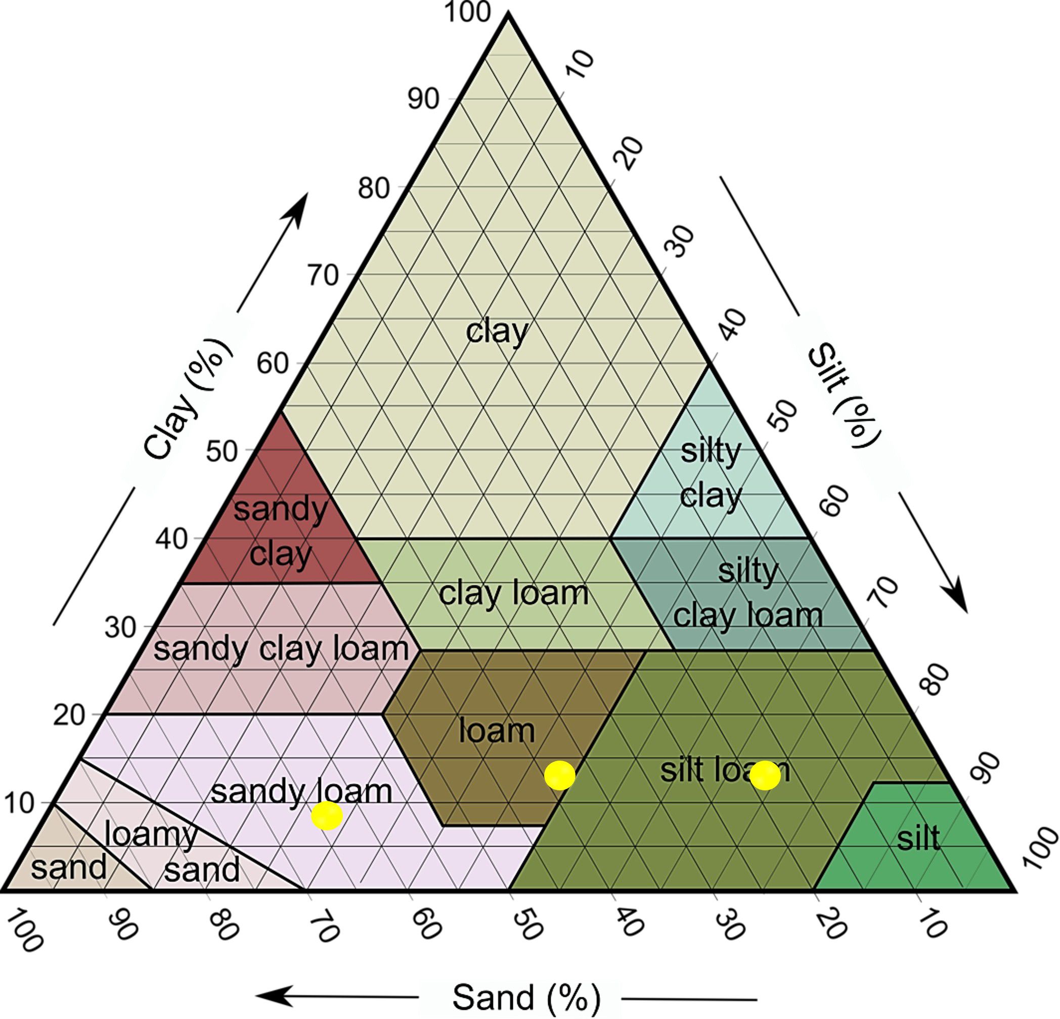
Figure 1. Soil texture classes (silt, clay, and sand) for each studied soil.

Table 1

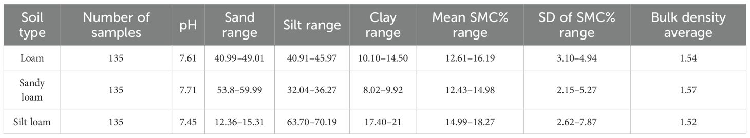
Table 1. Soil property averages and range values in all studied soil types and depths with mean SMC values and standard deviation.

2.2 Gravimetric technique for soil moisture content measurements

A total of 405 soil samples were collected from depths of 5, 20, 40, 60, and 80 cm on three soil types: loam, silt loam, and sandy loam, with 135 samples each. Sampling locations were determined according to the USDA’s recommended procedures (36), ensuring representative and systematic coverage across the three soil textures, loam, sandy loam, and silt loam (Figure 2A). Each sampling point shown in the figure represents measurements taken at all five specified depths. The samples were collected using an auger on 10 different dates every 2 weeks (June 1–15, July 2–15, August 4–21, September 5–20, and October 3–18). They were collected from the field in the same sensor’s locations from a 1-m² circle around the sensor. The samples were saved in plastic bags to maintain their moisture content before being moved to the laboratory. After that, they were placed in pre-weighed containers and weighed using a digital scale to record their initial weights. The samples were then transported to the laboratory and oven-dried at 105°C for 24 h (37, 38). After drying, the samples were weighed again to obtain their post-drying weights. Finally, the empty weights of the soil moisture containers were measured. SMC based on dry weight was calculated using Equation 1:

Figure 2

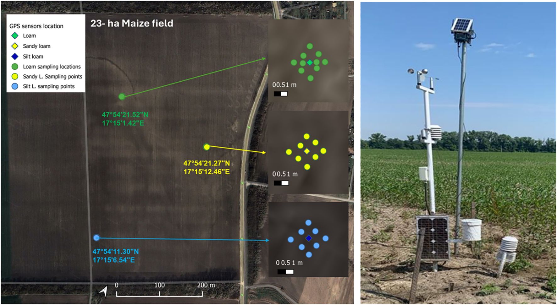
Figure 2. (A) Sensor station’s locations at the field with soil types, GPS coordinates, and spatial distribution of sensor stations and corresponding sample locations within each identified soil type. (B) IoT sensor stations based in the field (wind sensor, precipitation sensor, solar radiation sensor, humidity sensor, and temperature sensor).

$\begin{array}{ll}\theta =\frac{Mw}{Md}\times 100& (1)\end{array}$

where:

● θ = soil moisture content (%)

● Mw = mass of water (g) = (wet weight – dry weight)

● Md = mass of dry soil (g)

2.3 Data preparation and processing

The dataset was carefully prepared to address incorrect, missing, or hard-to-interpret values that could lead to overfitting or inaccurate, or deceptive results from the algorithm. Data preparation, including data transformation and statistical testing, was carried out using Python (version 3.10.12) (39) to ensure that there were no missing or zero values and to verify that the data types entering the model were accurate and consistent; in addition, basic statistical analyses including variation analysis and means calculations were conducted using Python. Additionally, dates and soil types were defined in the model to replace numerical values with appropriate date formats and soil type names. Following the data preparation, three ML algorithms—RFR, LSTM, and XGBoost—were employed to predict SMC in all soil types and depths. The dataset, which contained over 6,500 records collected from SMC measurements and meteorological data, was split into two parts: 80% for model training and 20% for testing. Each algorithm utilizes six inputs (SMC%, precipitation, humidity, temperature, solar radiation, and wind speed).

2.4 AI-based models

2.4.1 Random forest regression

The RFR is an approach based on classification trees. Belgiu and Drăguţ (40) described the primary phases of the RFR algorithm as follows:

1. Randomly selecting a subset of the original training set with replacement.

2. Using the subset to build the regression tree model.

3. Averaging the results of all trees to produce the final prediction.

The key hyperparameters used were as follows:

- n_estimators: defines the number of trees.

- random_state = 42: ensures reproducibility.

- max_leaf_nodes: limits the number of terminal nodes or leaves in each tree, which can reduce overfitting.

In general, the samples were divided, with approximately two-thirds of the dataset (in-bag data) for training samples and the remaining part for validation samples [out-of-bag (OOB) data] (Figure 3) (41). The RFR model was implemented using Python with the Pandas, NumPy, Matplotlib, and Scikit-learn libraries.

Figure 3

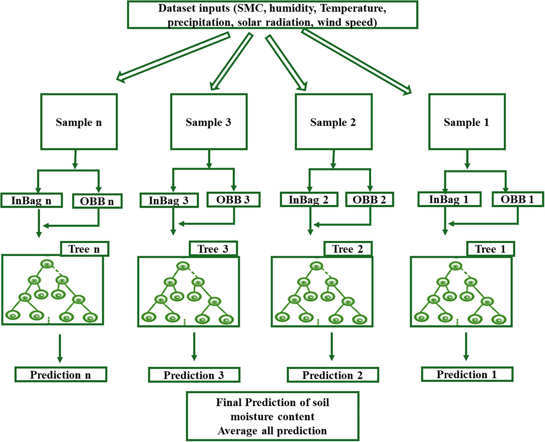
Figure 3. Random forest regression (RFR) model architecture.

2.4.2 Long short-term memory architectures

LSTM networks are a type of recurrent neural network (RNN) architecture designed to address the vanishing gradient problem and effectively capture long-range dependencies in sequential data. In the RNN model, the output from the previous step is utilized as input for the next step. This model is well-suited for predicting SMC as it can model time-series data, such as meteorological variables, and their impact on soil moisture trends.

The LSTM model used in this study comprises two layers (Figure 4): The first LSTM layer has 50 units and return_sequences=True, allowing the output to be passed to the second LSTM layer. The second LSTM layer also has 50 units. The hyperparameters utilized were epochs (number of training cycles) and batch_size. The optimizer used was Adam, with a mean_squared_error loss function. The output was generated by a dense layer with a single unit. The input data were normalized using the MinMaxScaler, ensuring all values were scaled between 0 and 1. The data were reshaped into a 3D array (samples, time steps, and features) before being input into the LSTM layers. The LSTM model was constructed and trained using Python with Pandas, NumPy, Matplotlib, and Scikit-learn libraries, in addition to TensorFlow for the LSTM layers.

Figure 4

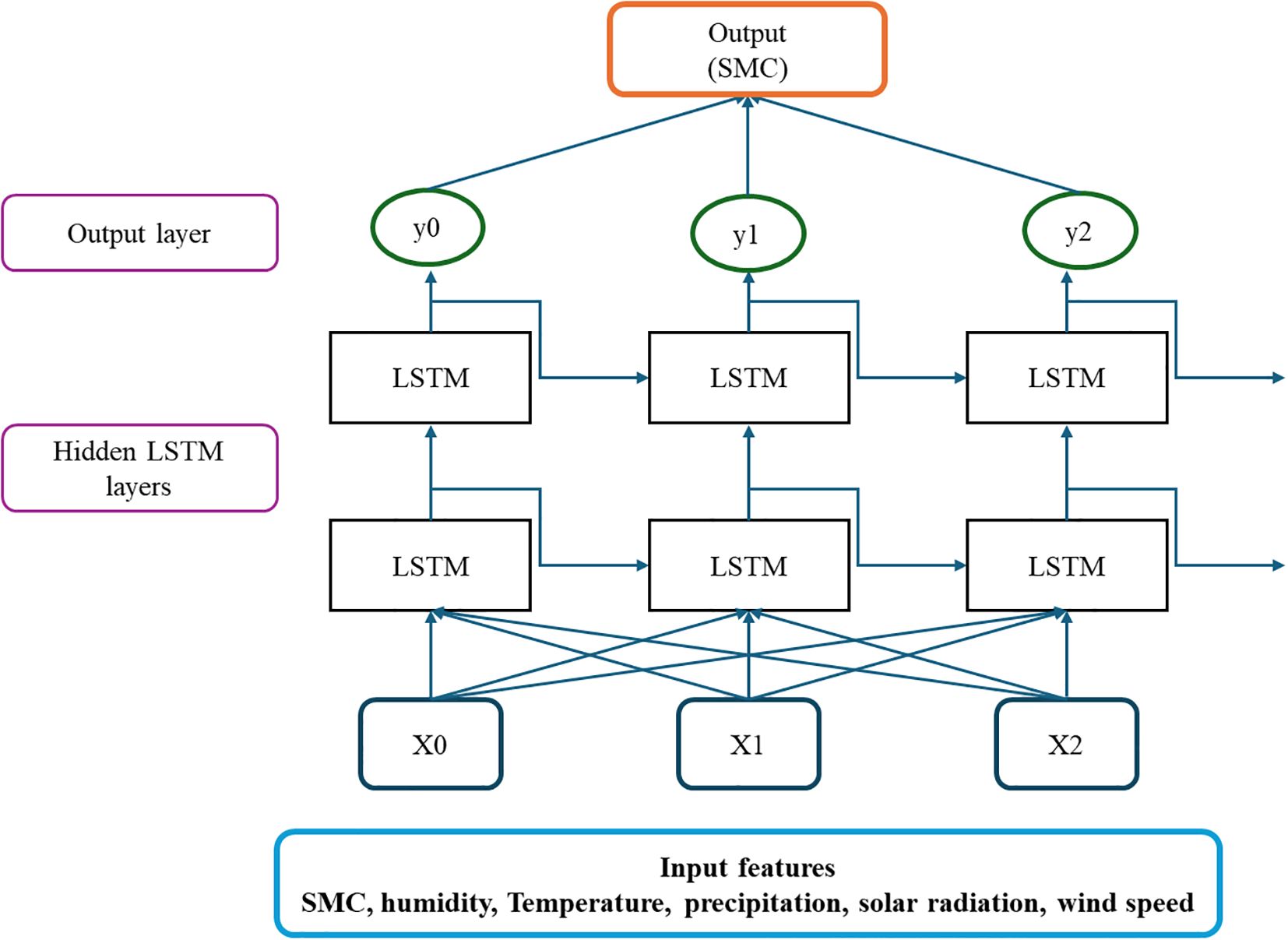
Figure 4. Diagram of LSTM layers.

2.4.3 XGBoost

The XGBoost technique, developed by Chen and Guestrin (42), is a powerful method for supervised learning that can handle regression and classification issues effectively. The XGBR algorithm is widely used in data mining due to its quick execution speed achieved by parallelization, out-of-core computation, and cache optimization. Data scientists appreciate its adaptability to different environments and excellent performance in small-scale data analysis. In a recent study, XGBoost was used to predict SMC using meteorological and soil moisture input features. The model’s hyperparameters were fine-tuned using a grid search to identify the best configuration, including n_estimators, learning_rate, and max_depth. The optimal configuration was selected using fivefold cross-validation to ensure the model’s ability to generalize well in studied soil types and depths. The flowchart for the XGBoost model is summarized in Figure 5. The XGBoost model was developed and trained using Python, along with libraries such as Pandas, NumPy, Matplotlib, and the XGBoost library.

Figure 5

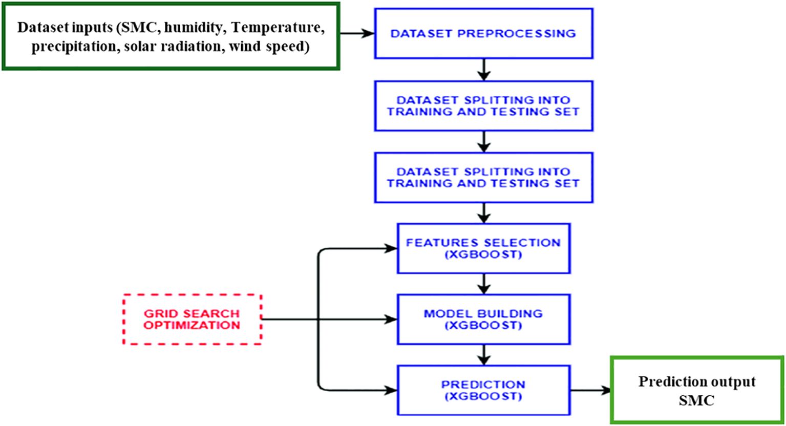
Figure 5. Flowchart of the XGBoost model.

2.5 Performance evaluation measures

Four indicators were calculated to quantify the performance of the different models.

Mean square error (MSE): The MSE is the average of the squared differences between projected and observed. In other words, the MSE represents the variance of the mistake (43). It is calculated using Equation 2:

$\begin{array}{ll}\text{MSE}=\raisebox{1ex}{$1$}\!\left/ \!\raisebox{-1ex}{$n$}\right.{\displaystyle {\sum }_{t=1}^n{(y_t-\widehat{y}t)}^2}& (2)\end{array}$

where y_t is the ground truth, and $\widehat{y}$ represents the mean of the predicted values.

Root mean square error (RMSE): It captures the typical difference between predicted and observed values (43). It is calculated by taking the square root of the MSE. Unlike MSE, RMSE is measured in the same units as the original data, making it easier to interpret. Since RMSE considers squared differences, it emphasizes larger deviations from predictions. This makes RMSE valuable when minimizing significant discrepancies is critical (Equation 3).

$\begin{array}{ll}\text{RMSE}=\sqrt{\raisebox{1ex}{$1$}\!\left/ \!\raisebox{-1ex}{$n$}\right.{\displaystyle {\sum }_{t=1}^n{(y_t-\widehat{y}t)}^2}}& (3)\end{array}$

Mean absolute error (MAE) (43): It calculates the average of the absolute differences between predictions and actual observations (Equation 4):

$\begin{array}{ll}\text{MAE}=\raisebox{1ex}{$1$}\!\left/ \!\raisebox{-1ex}{$n$}\right.{\displaystyle {\sum }_{t=1}^n\left|y_t-\widehat{y}t\right|}& (4)\end{array}$

R-squared (R²): It is an indicator of statistical significance that compares the variation explained by the model to the total variance. Higher R² indicates less difference between real and projected values. It is calculated using Equation 5:

$\begin{array}{ll}{R}^2=1-\frac{{\sum }_{t=1}^n{(y_t-\widehat{y}t)}^2}{{\sum }_{t=1}^n{(y_t-\underset{\_}{y})}^2}& (5)\end{array}$

where y_i is the predicted value, y_t is the ground truth, and $\widehat{y}$ represents the mean of the predicted values.

2.6 Feature importance analysis

Feature importance analysis was conducted for each ML model to evaluate and compare the contribution of studied meteorological variables to SMC prediction. For RFR, the Gini-based significance approach from scikit-learn was used to calculate the average reduction in error supplied by each feature across the forest (44, 45). In the LSTM model (an RNN model implemented in TensorFlow/Keras), feature importance is not inherently provided; thus, a model-agnostic permutation importance approach was applied and calculated by assessing the increase in MSE after shuffling each predictor variable in the validation dataset. Finally, with XGBoost, the built-in gain-based feature importance measure was utilized to calculate the cumulative improvement in the model’s accuracy when splitting by each feature (46). All analyses were conducted in Python and all feature importance results were computed separately for each soil type, depth, and model.

3 Results and discussion

3.1 Statistical analysis results for the three soil types

After analyzing 405 SMC% measurements in three types of soil and five depths over the maize vegetation season, the results shown in Figure 6 demonstrate that silt loam soil has the highest mean SMC, ranging from 14.99% to 18.27% due to its balanced sand, silt, and clay particle texture, which maximizes water retention (47), with the highest SMC (27.23%) recorded at 60 cm depth and the highest variability in the deeper layers (60 and 80 cm). The mean moisture content of loam soil varied from 12.61% to 16.19% at the five depths, with larger variability shown at deeper layers (60 and 80 cm), and maximum SMC value was at 20 cm depth with 22.1%. Sandy loam soil had a lower mean moisture content than loam soil due to its higher sand content, which decreased water retention, and the mean SMC ranged between 12.43% and 14.98%, with the highest SMC (20.77%) recorded at 80 cm depth. The low moisture content of sandy loam resulted in little variation among the five depths due to the high sand content, which reduces the water holding capacity and effect on soil water movement and dynamics through the soil layers (48). The highest SMC values and variability in deeper soil layers across all soil types are attributed to higher water retention capacity at depth compared with surface layers in the studied area (49). This variation in SMC% highlights the need to consider soil types and depth when monitoring soil moisture dynamics, as these factors had a significant impact on SMC variation (50). These results could be used in optimizing irrigation management, which will reduce water waste and enhance sustainability.

Figure 6

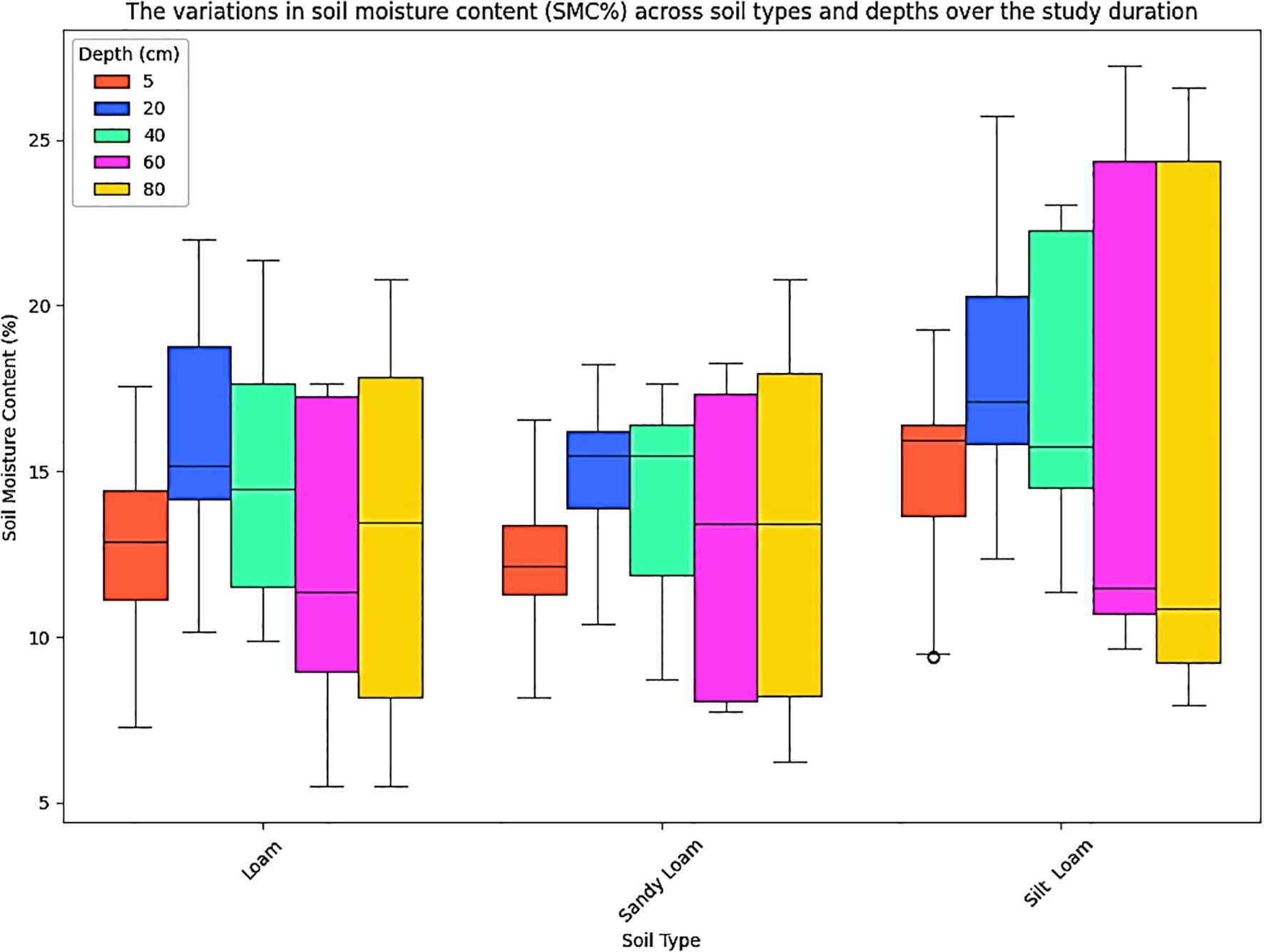
Figure 6. Soil moisture content variation in three soil types at five different depths.

3.2 Validation and predictive performance in studied soil types and depths

The performance of the three models (RFR, XGBoost, and LSTM) in predicting SMC in the studied soil types and depths resulted in several findings (Table 2).

Table 2

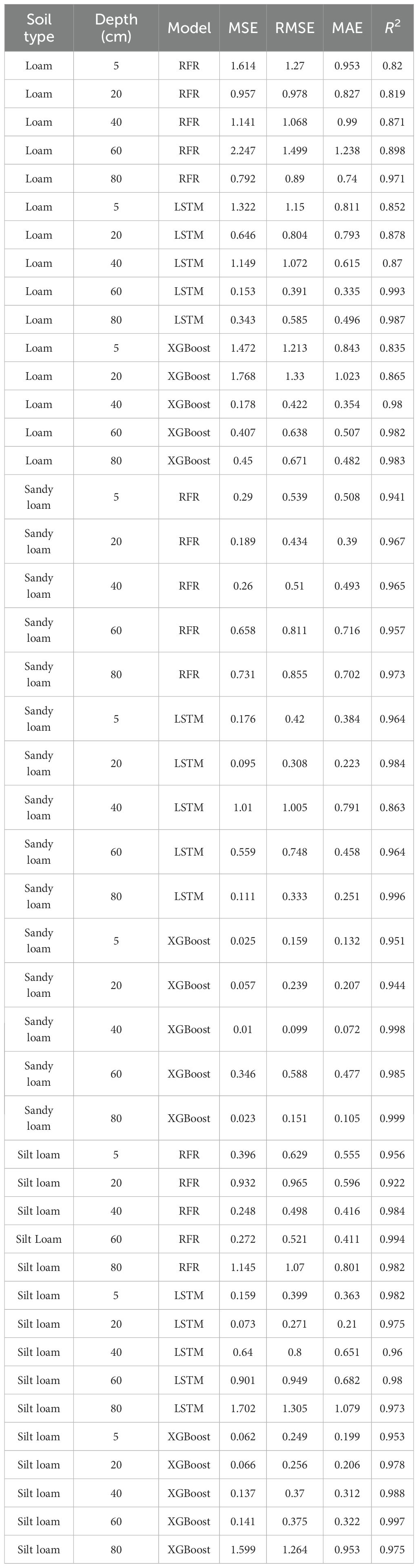
Table 2. Performance metrics evaluation results of the three used models across studied soil types and depths.

Among the three models, the RFR model consistently demonstrated the most robust and generalizable performance in all studied soil types and depths. For instance, in loam soil, at depths of 80 and 20 cm, the model achieved the lowest RMSE values of 0.89 and 0.98 and MAE values of 0.74 and 0.89, respectively. Figure 7 highlighted the model’s ability to highly accurately predict SMC at different layers in loam soil. In sandy loam soil, RFR performed best at depths of 20, 40, and 5 cm with RMSE values of 0.43, 0.51, and 0.54, respectively, and MAE values of 0.39, 0.49, and 0.51, respectively. Additionally, the model performed accurately in silt loam soil at 40- and 60-cm depths with RMSE values of 0.49 and 0.52, and MAE values of 0.42 and 0.41, respectively. These results align with the results of Cheng et al. (10) and Draper et al. (51) and suggest that RFR accurately captures the variation in SMC in all studied soil types and depths (52).

Figure 7

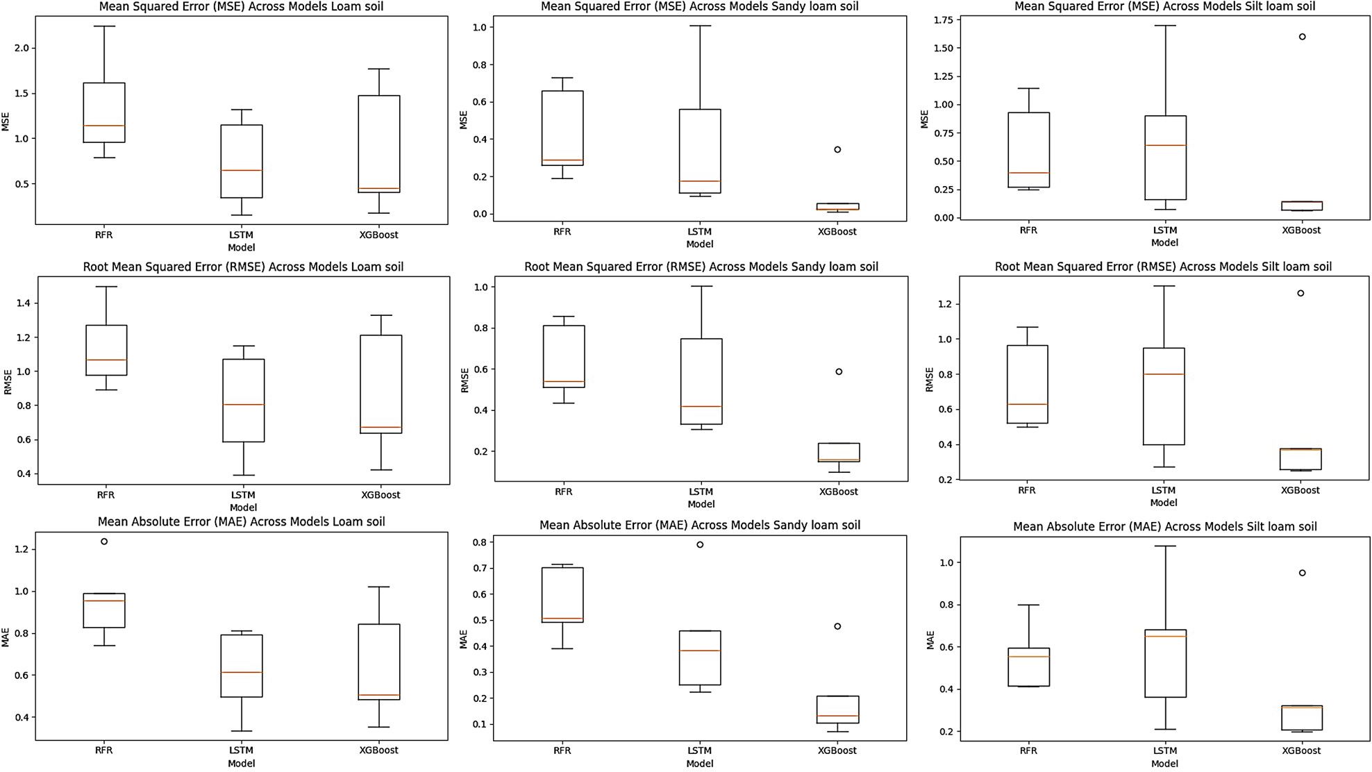
Figure 7. Predictive performance and validation results (MSE, RMSE, and MAE) for all soil types.

On the other hand, the LSTM models also showed promising results, particularly at shallow to moderate depths (20, 40, and 60 cm) and at all soil types where the meteorological factors have more impact on SMC variation at these layers, while it performed less consistently compared with RFR. For instance, in loam soil, at depths of 60 and 20 cm, the model achieved the lowest RMSE values of 0.39 and 0.80 and MAE values of 0.34 and 0.79, respectively. Figure 7 highlighted the model’s ability to accurately predict SMC at different layers in loam soil. In sandy loam soil, LSTM had the best performance at depths of 20 and 5 cm with RMSE values of 0.31 and 0.42, respectively, and MAE values of 0.22 and 0.38, respectively. In addition, in silt loam soil, the lowest errors were at 20- and 5-cm depths with RMSE values of 0.27 and 0.34, and MAE values of 0.21 and 0.36, respectively (Figure 7), aligning with the results of Filipović et al. (3) and Park et al. (53). These findings indicate that the LSTM model demonstrates promising performance in predicting SMC, and the ability to accurately predict SMC, especially at shallower to moderate depths where the impact of environmental factors is higher than deeper layers (28).

The XGBoost models that offered a high performance in capturing complex and nonlinear relations performed well in different soil types and depths especially the shallower depths. The model showed a high accuracy at 40- and 60-cm depths in loam soil with the lowest RMSE values of 0.422 and 0.638, and MAE values of 0.354 and 0.507, respectively (Figure 7). In sandy loam, the best errors were at depths of 40 and 5 cm where XGBoost had RMSE values of 0.099 and 0.159, and MAE values of 0.072 and 0.132, respectively, which considers higher performance in shallow depths compared with the results by Ren et al. (27), where the highest RMSE was 11.11 and MAE was 4.87. Similarly, in silt loam soil, it performed well at 5 and 20 cm with RMSE values of 0.249 and 0.256, and MAE values of 0.199 and 0.206, respectively. The acceptable threshold for RMSE value is 10% (54). During the experiment period, the models predicted SMC with RMSE values ranging from 0.24% to 0.9%. These low MSE and RMSE values, along with a high R² value, suggest that these models can effectively predict SMC as an alternative to classic empirical equations (55).

The variation in the measured parameters between deeper layers and upper layers is caused by different influencing factors. Shallower depths (5–20 cm) are directly affected by weather conditions such as precipitation and humidity, making it easier for the model to predict SMC accurately with high-quality data. On the other hand, deeper layers (40–80 cm) are influenced by factors like surface water dynamics, soil structure, and other soil properties, making it more complex for the model to accurately predict SMC in these layers (56, 57) and emphasizing the need to consider more features in model training for deeper soil layers.

The RFR exhibited consistent prediction accuracy with high R² values. In loam soil, RFR achieved R² values ranging from 0.820 to 0.971, with the highest R² at 80 cm depth. Similarly, in sandy loam soil, RFR performed well, with R² values ranging from 0.941 to 0.973, peaking at 20 cm depth. Moreover, in silt loam soil, the model had R² values ranging from 0.956 to 0.994, with the highest R² at 60 cm depth (Figure 8). These results align with the findings of Cheng et al. (10) and Zhao et al. (58) and demonstrate that the RFR model offered the best generalization in the studied soil types and depths, especially the deeper layers where the impact of meteorological factors is less, and SMC is affected by other factors such as soil properties and components (11). On the other hand, the LSTM model showed promising accuracy results, especially at shallower depths where the model achieved R² values in loam soil ranging from 0.852 to 0.987, with the highest R² found at 60 cm depth. In sandy loam soil, LSTM performed well with R² values ranging from 0.964 to 0.996, peaking at 80 cm depth. Similarly, in silt loam soil, R² values varied from 0.982 to 0.980 (Figure 8), with the best R² found at 60 cm depth; similar results were achieved in other research studies (28, 59). These findings indicate that LSTM models can accurately represent the temporal dynamics of SMC in various soil types and depths, particularly at shallow to intermediate depths, compared to other models (60). However, LSTM performance decreased as depth increased in all soil types.

Figure 8

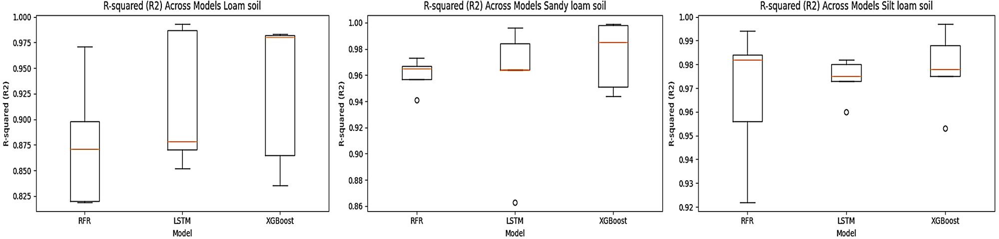
Figure 8. Accuracy performance evaluation of the RFR, LSTM, and XGBoost in all soil types.

In loam soil, XGBoost had R² values ranging from 0.835 to 0.983, with the highest R² at 40 cm depth, while in sandy loam soil, R² values ranged from 0.951 to 0.999, with the highest value at 40 cm depth. Similarly, in silt loam soil, R² values varied from 0.953 to 0.997, with the best R² found at 60 cm depth (Figure 8). These findings indicate that XGBoost models may accurately capture the complicated interactions between SMC and environmental variables in a variety of soil types and depths. However, XGBoost’s performance decreased at deeper depths in loam and silt loam soils (27, 61). The results showed that the RFR model had the most consistent performance in all soil types and depths in comparison with XGBoost that performed best at shallower depths (5 to 40 cm) and LTSM in shallow to moderate layers (5, 20, 40, and 60 cm). In addition, RFR offered the best generalization capacity. These findings highlighted the need for further improvements for the models to increase accuracy in the deep oil layers where factors other than meteorological data have a significant impact on soil moisture dynamics.

3.3 The training and validation loss behaviors of models in studied soil types and depths

The learning curves of the LSTM model indicated a decrease in loss values (MSE) with increasing epochs, particularly between 600 and 800, suggesting improved model generalization. However, there were slight variations in loss curves, indicating potential moderate overfitting at specific depths and soil types, such as 60 and 80 cm in loam soil (Figure 9) and 20, 40, and 80 cm in silt loam soil (Figure 10) (62). On the other hand, when the number of trees increased to 200, both the RFR and XGBoost models demonstrated decreasing loss values, showing improved model performance with increased complexity (63). However, deviations from this trend were observed, particularly in XGBoost models for sandy loam soil at 5 and 40 cm depth (Figure 11) and silt loam soil at 20 and 40 cm depth (Figure 10), where loss values slightly increased with the number of trees, indicating potential instability or poor performance under certain conditions. Overall, while all models showed improved performance with a higher number of epochs for LSTM (62) and greater model complexity for RFR and XGBoost (63), the LSTM model consistently outperforms and stabilizes in all studied soil types and depths.

Figure 9

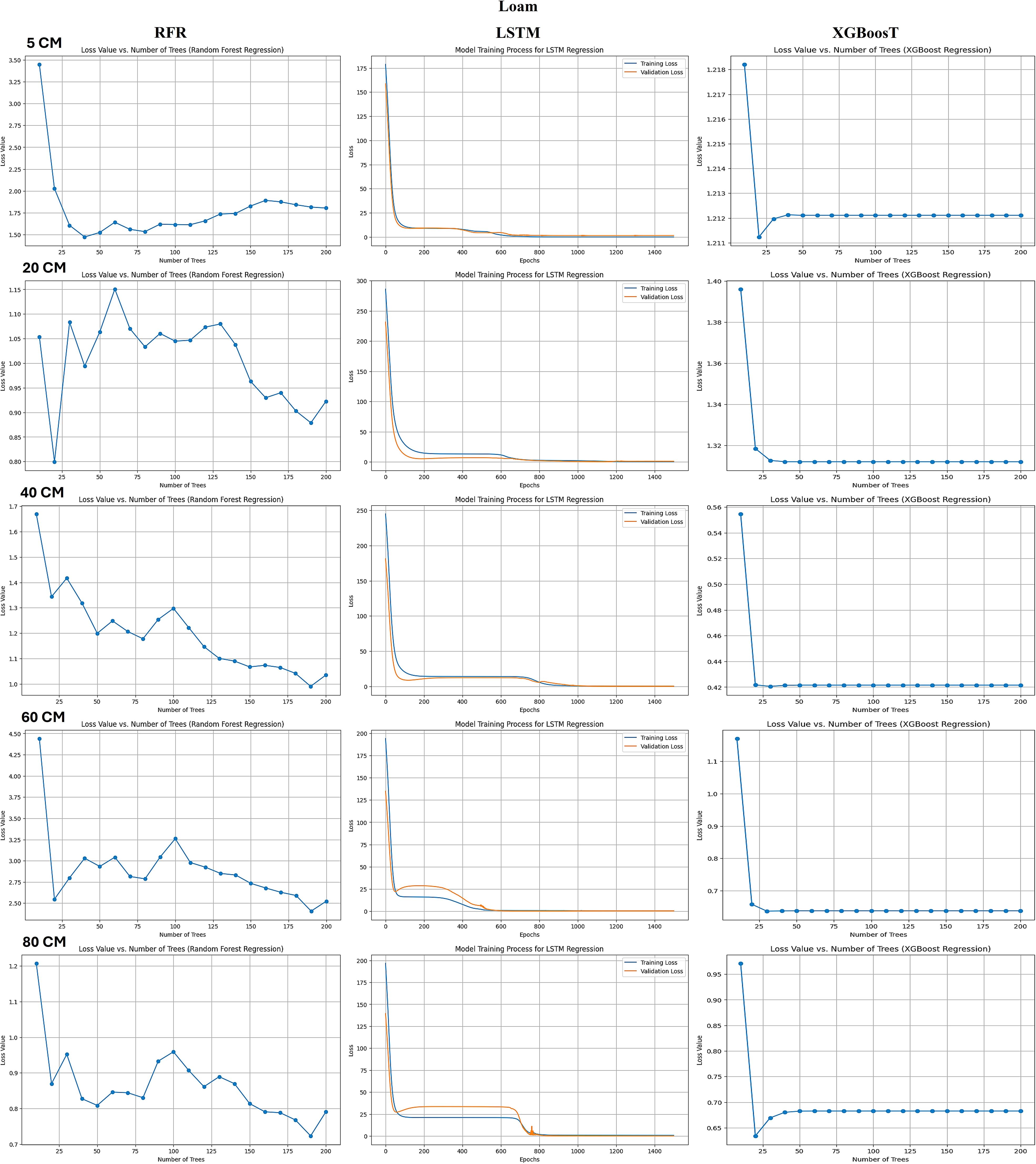
Figure 9. The loss value vs. the number of trees and epochs for RFR, XGBoost, and LSTM at various depths in loam soil.

Figure 10

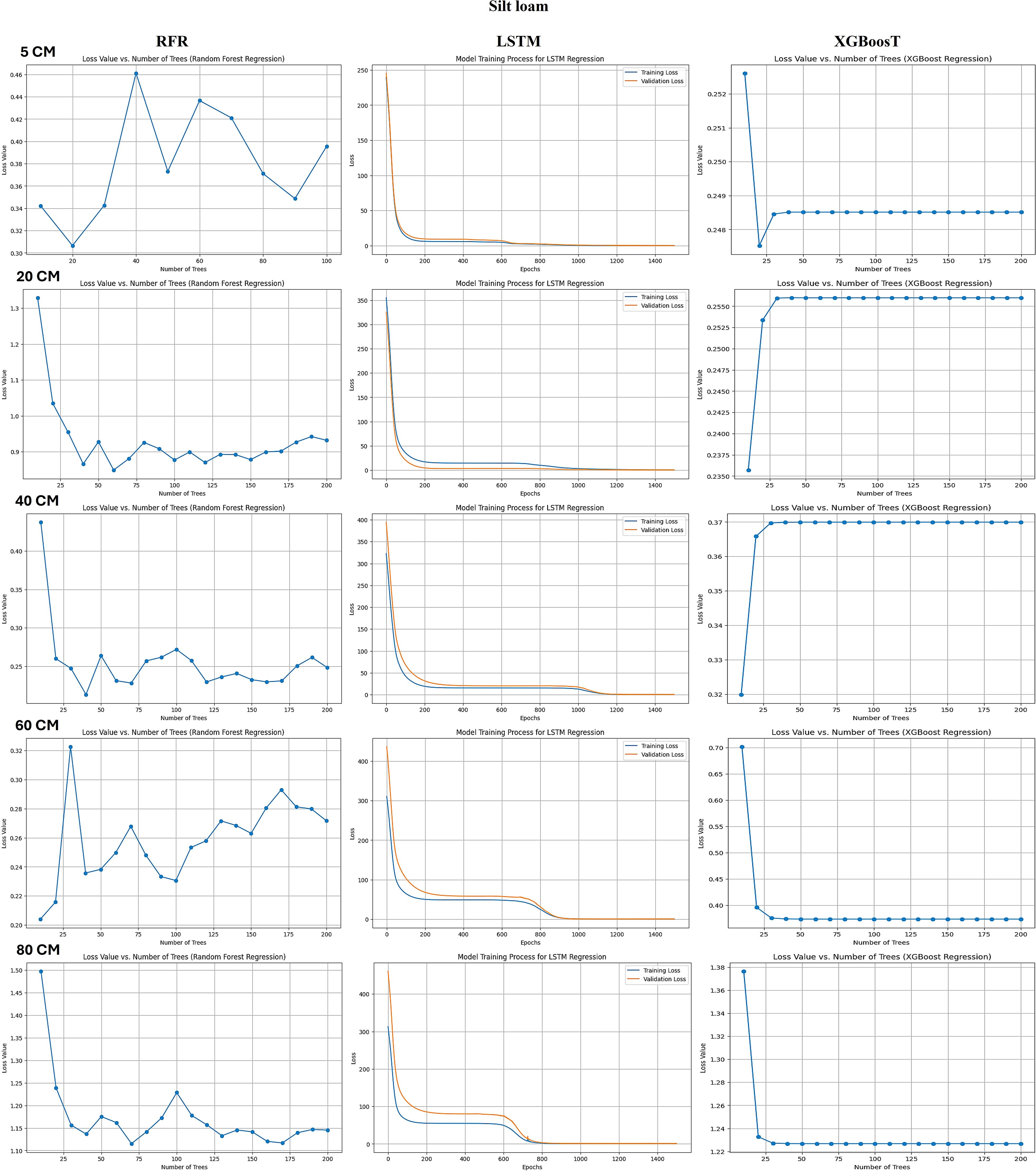
Figure 10. The loss value vs. the number of trees and epochs for RFR, XGBoost, and LSTM at various depths in silt loam soil.

Figure 11

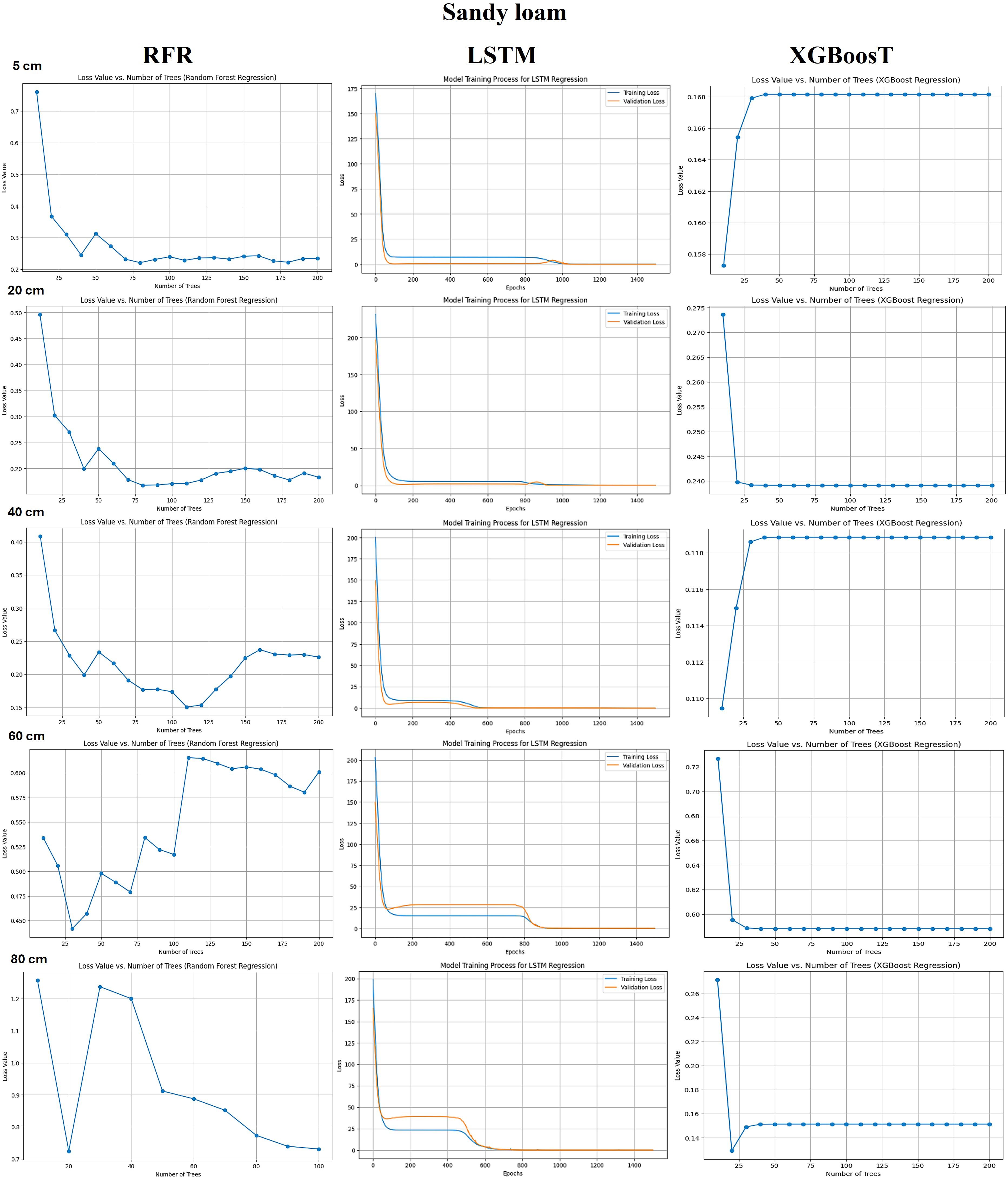
Figure 11. The loss value vs. number of trees and epochs for RFR, XGBoost, and LSTM at various depths in sandy loam soil.

3.4 Comparison of measured and predicted SMC% values

The comparison between measured and predicted SMC% values at different depths in all soil types provides insight into the models’ predictive performance. The results show the model’s ability to accurately represent underlying patterns and variability in SMC at various depths and soil types. The close agreement between measured and predicted values indicates that the modeling approaches accurately predict SMC% (see Figure 12), and the mean measured and predicted values are provided in Appendix A. Compared with previous research by Alibabaei et al. (28) and Ren et al. (27), which developed different models to predict SMC, this research combines multiple soil layers’ SMC prediction with three AI-based ML models in three soil types, with the use of gravimetric data for more accurate validation and learning; the use of in situ IoT sensors data and high temporal resolution allows for more robust performance of the model than the use of only satellite images for model training. Thus, the soil-specific and depth-specific modeling achieved in this research is vital for precision irrigation management and drought monitoring. Variations between measured and predicted values, especially at certain depths or soil types, suggest many potentials for model development especially for deep soil layers (52, 55). Enhancing models’ generalizability and applicability could be done by considering extending the inputs with more variables such as different locations instead of only one location in this research, irrigations, evapotranspiration, vegetation indices from more vegetation seasons, and utilizing more soil properties such as soil texture and organic matter content.

Figure 12

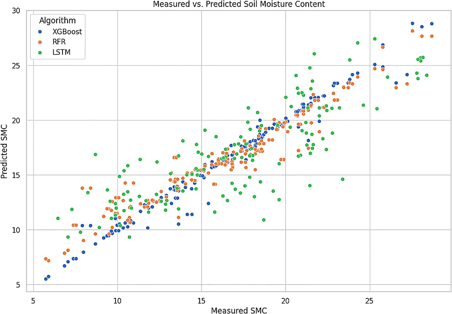
Figure 12. Measured and predicted soil moisture content results by the three ML models (RFR, XGBoost, and LSTM).

3.5 Feature importance analysis results

The feature importance analysis revealed both common patterns and significant differences in how the three models prioritize the environmental variables. Overall, the studied meteorological data have contributed to SMC prediction, but solar radiation consistently showed as the most effective predictor, particularly for SMC in deeper soil layers (40 to 80 cm), achieving average values ranging from 0.4 to 0.85 across three soil types and five depths with highest values of impact on silt loam with three models (0.8 with RFR, 0.79 with XGBoost, and 0.7 in LSTM) (Figure 13). This result demonstrates that evaporative demand caused by solar energy input is a dominating component driving soil moisture variability at depth, which is consistent with previous research indicating that solar radiation and temperature strongly influence soil water evaporation and drying (64, 65). On the other hand, precipitation had an important role in SMC prediction, especially at surface layer 5 cm in the three soil types with average values of 0.14 in RFR, 0.4 in XGBoost, and 0.25 in LSTM. These results emphasize the role of precipitation in increasing the SMC in surface layers (66). Humidity, temperature, and wind speed had varied importance among models, soil types, and depths. While analysis results showed the relatively high importance of humidity and wind speed in loam and silt loam soils, particularly at surface layers 5 and 20 cm with RFR and LSTM models, temperature had high importance value in sandy loam soil with the XGBoost model achieving values of 0.17 and 0.44 at 5- and 20-cm depths, respectively.

Figure 13

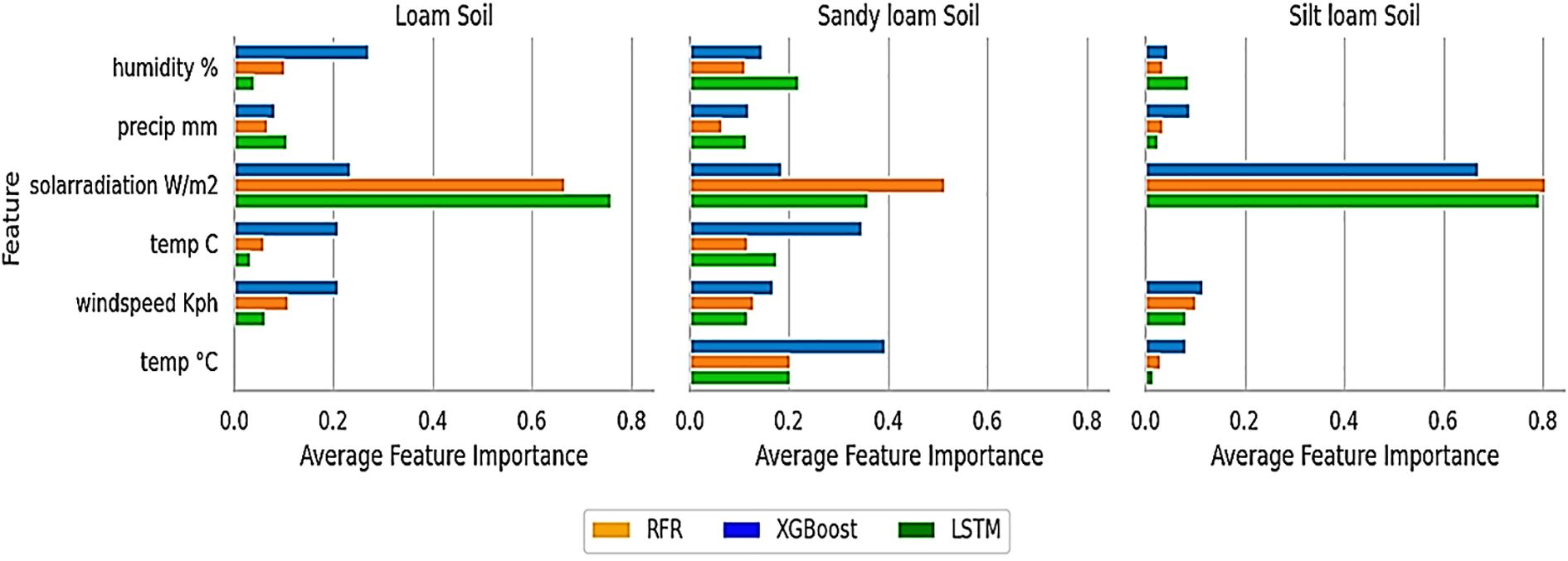
Figure 13. Average feature importance value results by the three ML models (RFR, XGBoost, and LSTM) per soil type across all depths.

These variations represent each algorithm’s learning method. LSTMs, which are designed to capture temporal patterns and lag effects, may prioritize characteristics such as temperature that represent long-term environmental influences. RFR and XGBoost, on the other hand, use threshold-based decision rules and prioritize features that bring quick advances in predictive accuracy, such as recent precipitation or current wind speeds. Despite these model-specific variations, solar radiation and precipitation were the two most important variables impacting SMC across depths, soil types, and models. These findings are consistent with hydrological SMC principles, in which precipitation determines water input and solar radiation with temperature causing evapotranspiration and moisture loss (67). Overall, the feature importance results showed that the ML models effectively captured the key hydrological factors that influenced soil moisture dynamics. In particular, the ability to quantify and rank the impact of different predictors provides a solid base for optimizing irrigation systems. By identifying the key variables impacting SMC at certain depths and soil types, this study allows for data-driven decisions that support site-specific irrigation scheduling, reduce water use waste, and improve resource use efficiency. Additionally, feature importance analysis not only enhances model interpretability but also directly contributes to the objectives of sustainable water management and precision crop production. However, it is important to acknowledge that the influence of environmental predictors varies notably across soil types and depths. This highlights the need to develop soil-specific and depth-specific models that account for these variations by selecting key drivers tailored to each scenario. Additionally, the current study was limited to data from a single location and one growing season, which may affect the generalizability of the results to other regions or climatic conditions. Incorporating multi-season and multi-location datasets in future research would improve the robustness and transferability of the models. Furthermore, integrating intrinsic soil properties such as the percentages of sand, silt, and clay, along with other relevant variables like vegetation indices and organic matter into the predictive framework, could enhance model accuracy and adaptability. Expanding the comparison to include additional ML algorithms and larger datasets will also be essential to strengthen performance and ensure scalability for broader precision irrigation applications.

4 Conclusions

The research introduced soil-specific and depth-specific modeling for SMC prediction at three different soil types and five depths (5, 20, 40, 60, and 80 cm) using three ML models (RFR, XGBoost, and LSTM). The results showed that SMC varied in the studied soil types, with sandy loam soil exhibiting less variance and silt loam and loam soils showing higher variability across depths. This emphasizes the importance of considering both soil type and depth when monitoring SMC.

RFR performed the best in all studied soil types and depths, particularly in capturing soil moisture variability in deeper soil layers (60 and 80 cm). LSTM performed well at shallower to moderate depths (5 to 60 cm) with less accuracy in deeper soil layers. On the other hand, XGBoost achieved high accuracy in predicting SMC in shallower depths, particularly in sandy loam soil due to its ability to model complex interactions between meteorological inputs and soil moisture dynamics. The differences between measured and predicted values provide opportunities for model modification and validation, especially for deeper layers and the need to enhance the generalizability and applicability of models by considering increasing inputs for model training with more variables such as different locations, irrigations, evapotranspiration, vegetation indices, and soil properties, as well as highlighting the fact that each soil type and depth could be modeled with different algorithms. The feature importance analysis results further demonstrated the dominant role of solar radiation and precipitation, emphasizing their significant influence on soil moisture dynamics.

These findings highlight the practical importance of these models in agricultural and environmental management. By accurately predicting SMC, these models could enhance water-use efficiency, optimize irrigation schedule, and improve understanding of soil moisture dynamics for ecosystem management. The study also demonstrates the potential for expanding these models to predict SMC in different regions, offering valuable insights for decision-makers in agriculture, hydrology, and enhancing the sustainability that aligned with Sustainable Development Goal 6 (SDG6) (sustainable management of water). While the models demonstrated strong predictive performance, their application is currently limited to a single site and one growing season. Future research should focus on expanding datasets across multiple locations and seasons, integrating additional soil properties and vegetation indices, and testing a wider range of algorithms to enhance accuracy, adaptability, and scalability for broader precision irrigation applications.

Data availability statement

The raw data supporting the conclusions of this article will be made available by the authors, without undue reservation.

Author contributions

TA: Writing – review & editing, Writing – original draft, Formal Analysis, Methodology. MN: Writing – review & editing, Supervision. AS: Validation, Writing – review & editing. NA: Writing – review & editing. OH: Writing – review & editing. AN: Methodology, Conceptualization, Writing – review & editing, Writing – original draft.

Funding

The author(s) declare financial support was received for the research and/or publication of this article. The research was supported by the EKÖP-24-3-I-SZE-107 University Research Fellowship Program of the Ministry for Culture and Innovation from the Source of the National Research, Development and Innovation Fund; the “Precision Bioengineering Research Group” supported by the “Széchenyi István University Foundation”; and the János Bolyai Research Scholarship (Bo/00578/24) of the Hungarian Academy of Sciences. TKP2021-NKTA-32 has been implemented with the support provided by the Ministry of Culture and Innovation of Hungary from the National Research.

Conflict of interest

The authors declare that the research was conducted in the absence of any commercial or financial relationships that could be construed as a potential conflict of interest.

Generative AI statement

The author(s) declare that no Generative AI was used in the creation of this manuscript.

Any alternative text (alt text) provided alongside figures in this article has been generated by Frontiers with the support of artificial intelligence and reasonable efforts have been made to ensure accuracy, including review by the authors wherever possible. If you identify any issues, please contact us.

Publisher’s note

All claims expressed in this article are solely those of the authors and do not necessarily represent those of their affiliated organizations, or those of the publisher, the editors and the reviewers. Any product that may be evaluated in this article, or claim that may be made by its manufacturer, is not guaranteed or endorsed by the publisher.

References

1. Sundmaeker H, Verdouw C, Wolfert S, and Freire LP. Internet of food and farm 2020. In: Digitising the industry internet of things connecting the physical, digital and virtualWorlds. New York, USA: River Publishers (2022). p. 129–51.

Google Scholar

2. Kulmány IM, Bede-Fazekas Á, Beslin A, Giczi Z, Milics G, Kovács B, et al. Calibration of an Arduino-based low-cost capacitive soil moisture sensor for smart agriculture. J Hydrology Hydromechanics. (2022) 70:330–40. doi: 10.2478/johh-2022-0014

Crossref Full Text | Google Scholar

3. Filipović N, Brdar S, Mimić G, Marko O, and Crnojević V. Regional soil moisture prediction system based on Long Short-Term Memory network. Biosyst Eng. (2022) 213:30–8. doi: 10.1016/j.biosystemseng.2021.11.019

Crossref Full Text | Google Scholar

4. Stroobosscher ZJ, Athelly A, and Guzmán SM. Assessing capacitance soil moisture sensor probes’ ability to sense nitrogen, phosphorus, and potassium using volumetric ion content. Front Agron. (2024) 6:1346946. doi: 10.3389/fagro.2024.1346946

Crossref Full Text | Google Scholar

5. Bibek Acharya VS. COMPARATIVE ANALYSIS OF SOIL AND WATER DYNAMICS IN CONVENTIONAL AND SOD-BASED CROP ROTATION IN FLORIDA. Front Agron. (2025) 7:1552425. doi: 10.3389/fagro.2025.1552425

Crossref Full Text | Google Scholar

6. Luo W, Xu X, Liu W, Liu M, Li Z, Peng T, et al. UAV based soil moisture remote sensing in a karst mountainous catchment. Catena (Amst). (2019) 174:478–89. doi: 10.1016/j.catena.2018.11.017

Crossref Full Text | Google Scholar

7. Wang X, Liu H, Sun Z, and Han X. Soil moisture inversion based on multiple drought indices and RBFNN: A case study of northern Hebei Province. Heliyon. (2024) 10:e37426. doi: 10.1016/j.heliyon.2024.e37426

PubMed Abstract | Crossref Full Text | Google Scholar

8. Seneviratne SI, Corti T, Davin EL, Hirschi M, Jaeger EB, Lehner I, et al. Investigating soil moisture–climate interactions in a changing climate: A review. Earth Sci Rev. (2010) 99:125–61. doi: 10.1016/j.earscirev.2010.02.004

Crossref Full Text | Google Scholar

9. Mulla DJ. Twenty five years of remote sensing in precision agriculture: Key advances and remaining knowledge gaps. Biosyst Eng. (2013) 114:358–71. doi: 10.1016/j.biosystemseng.2012.08.009

Crossref Full Text | Google Scholar

10. Cheng M, Jiao X, Liu Y, Shao M, Yu X, Bai Y, et al. Estimation of soil moisture content under high maize canopy coverage from UAV multimodal data and machine learning. Agric Water Manag. (2022) 264:107530. doi: 10.1016/j.agwat.2022.107530

Crossref Full Text | Google Scholar

11. Lv C, Xie Q, Peng X, Dou Q, Wang J, Lopez-Sanchez JM, et al. Soil moisture retrieval over agricultural fields with machine learning: A comparison of quad-, compact-, and dual-polarimetric time-series SAR data. J Hydrol (Amst). (2024) 644:132093. doi: 10.1016/j.jhydrol.2024.132093

Crossref Full Text | Google Scholar

12. Holsten A, Vetter T, Vohland K, and Krysanova V. Impact of climate change on soil moisture dynamics in Brandenburg with a focus on nature conservation areas. Ecol Modell. (2009) 220:2076–87. doi: 10.1016/j.ecolmodel.2009.04.038

Crossref Full Text | Google Scholar

13. Gao L, Wang Y, Geris J, Hallett PD, and Peng X. The role of sampling strategy on apparent temporal stability of soil moisture under subtropical hydroclimatic conditions. J Hydrology Hydromechanics. (2019) 67:260–70. doi: 10.2478/johh-2019-0006

Crossref Full Text | Google Scholar

14. Meißl G, Klebinder K, Zieher T, Lechner V, Kohl B, and Markart G. Influence of antecedent soil moisture content and land use on the surface runoff response to heavy rainfall simulation experiments investigated in Alpine catchments. Heliyon. (2023) 9:e18597. doi: 10.1016/j.heliyon.2023.e18597

PubMed Abstract | Crossref Full Text | Google Scholar

15. Singh A, Gaurav K, Sonkar GK, and Lee C-C. Strategies to measure soil moisture using traditional methods, automated sensors, remote sensing, and machine learning techniques: review, bibliometric analysis, applications, research findings, and future directions. IEEE Access. (2023) 11:13605–35. doi: 10.1109/ACCESS.2023.3243635

Crossref Full Text | Google Scholar

16. Little M and Smith. A comparison of three methods of soil water content determination. South Afr J Plant Soil. (1998) 15:80–9. doi: 10.1080/02571862.1998.10635121

Crossref Full Text | Google Scholar

17. Wagner W, Lemoine G, and Rott H. A method for estimating soil moisture from ERS scatterometer and soil data. Remote Sens Environ. (1999) 70:191–207. doi: 10.1016/S0034-4257(99)00036-X

Crossref Full Text | Google Scholar

18. Cai Y, Zheng W, Zhang X, Zhangzhong L, and Xue X. Research on soil moisture prediction model based on deep learning. PloS One. (2019) 14:e0214508. doi: 10.1371/journal.pone.0214508

PubMed Abstract | Crossref Full Text | Google Scholar

19. Cheng M, Li B, Jiao X, Huang X, Fan H, Lin R, et al. Using multimodal remote sensing data to estimate regional-scale soil moisture content: A case study of Beijing, China. Agric Water Manag. (2022) 260:107298. doi: 10.1016/j.agwat.2021.107298

Crossref Full Text | Google Scholar

20. Zheng W, Zhangzhong L, Zhang X, Wang C, Zhang S, Sun S, et al. A review on the soil moisture prediction model and its application in the information system. Cham, Switzerland (2019). pp. 352–64. pp. 352–64. doi: 10.1007/978-3-030-06137-1_32.

Crossref Full Text | Google Scholar

21. Haddon A, Kechichian L, Harmand J, Dejean C, and Ait-Mouheb N. Linking soil moisture sensors and crop models for irrigation management. Ecol Modell. (2023) 484:110470. doi: 10.1016/j.ecolmodel.2023.110470

Crossref Full Text | Google Scholar

22. Liakos K, Busato P, Moshou D, Pearson S, and Bochtis D. Machine learning in agriculture: A review. Sensors. (2018) 18:2674. doi: 10.3390/s18082674

PubMed Abstract | Crossref Full Text | Google Scholar

23. Nyéki A, Kerepesi C, Daróczy B, Benczúr A, Milics G, Nagy J, et al. Application of spatio-temporal data in site-specific maize yield prediction with machine learning methods. Precis Agric. (2021) 22:1397–415. doi: 10.1007/s11119-021-09833-8

Crossref Full Text | Google Scholar

24. Ågren AM, Larson J, Paul SS, Laudon H, and Lidberg W. Use of multiple LIDAR-derived digital terrain indices and machine learning for high-resolution national-scale soil moisture mapping of the Swedish forest landscape. Geoderma. (2021) 404:115280. doi: 10.1016/j.geoderma.2021.115280

Crossref Full Text | Google Scholar

25. Carranza C, Nolet C, Pezij M, and van der Ploeg M. Root zone soil moisture estimation with Random Forest. J Hydrol (Amst). (2021) 593:125840. doi: 10.1016/j.jhydrol.2020.125840

Crossref Full Text | Google Scholar

26. Senanayake IP, Yeo I-Y, Walker JP, and Willgoose GR. Estimating catchment scale soil moisture at a high spatial resolution: Integrating remote sensing and machine learning. Sci Total Environ. (2021) 776:145924. doi: 10.1016/j.scitotenv.2021.145924

Crossref Full Text | Google Scholar

27. Ren Y, Ling F, and Wang Y. Research on provincial-level soil moisture prediction based on extreme gradient boosting model. Agriculture. (2023) 13:927. doi: 10.3390/agriculture13050927

Crossref Full Text | Google Scholar

28. Alibabaei K, Gaspar PD, and Lima TM. Modeling soil water content and reference evapotranspiration from climate data using deep learning method. Appl Sci. (2021) 11:5029. doi: 10.3390/app11115029

Crossref Full Text | Google Scholar

29. Paul S and Singh S. Soil moisture prediction using machine learning techniques. In: Proceedings of the 2020 3rd international conference on computational intelligence and intelligent systems. ACM, New York, NY, USA (2020). p. 1–7. doi: 10.1145/3440840.3440854

Crossref Full Text | Google Scholar

30. Kheimi M and Zounemat-Kermani M. Conventional and advanced AI-based models in soil moisture prediction. Phys Chem Earth Parts A/B/C. (2025) 139:103944. doi: 10.1016/j.pce.2025.103944

Crossref Full Text | Google Scholar

31. Sahour H, Gholami V, Torkaman J, Vazifedan M, and Saeedi S. Random forest and extreme gradient boosting algorithms for streamflow modeling using vessel features and tree-rings. Environ Earth Sci. (2021) 80:747. doi: 10.1007/s12665-021-10054-5

Crossref Full Text | Google Scholar

32. Neményi M, Kovács AJ, Oláh J, Popp J, Erdei E, Harsányi E, et al. Challenges of sustainable agricultural development with special regard to Internet of Things: Survey. Prog Agric Eng Sci. (2022) 18:95–114. doi: 10.1556/446.2022.00053

Crossref Full Text | Google Scholar

33. Alahmad T, Neményi M, and Nyéki A. Applying ioT sensors and big data to improve precision crop production: A review. Agronomy. (2023) 13:2603. doi: 10.3390/agronomy13102603

Crossref Full Text | Google Scholar

34. USDA. ND. Natural Resources Conservation Service. Soil classification (2020). Available online at: https://www.nrcs.usda.gov/wps/portal/nrcs/main/soils/survey/class/ (Accessed July 29, 2024).

Google Scholar

35. Milics G, Kovács AJ, Pörneczi A, Nyéki A, Varga Z, Nagy V, et al. Soil moisture distribution mapping in topsoil and its effect on maize yield. Biol (Bratisl). (2017) 72:847–53. doi: 10.1515/biolog-2017-0100

Crossref Full Text | Google Scholar

36. USDA. Field book for describing and sampling soils V4.0. United States Department of Agriculture, Washington DC, USA: USDA (2024). Available online at: https://www.nrcs.usda.gov/resources/guides-and-instructions/field-book-for-describing-and-sampling-soils.

Google Scholar

37. Dirksen C. Soil physics measurements. Stuttgart, Germany: Catena Verlag (1999).

Google Scholar

38. Shukla A, Panchal H, Mishra M, Patel PR, Srivastava HS, Patel P, et al. Soil moisture estimation using gravimetric technique and FDR probe technique: a comparative analysis. Am Int J Res Form. Appl Nat Sci. (2014) 8:89–92. doi: 10.13140/RG.2.2.28776.70405

Crossref Full Text | Google Scholar

39. Python Software Foundation. Python Language Reference, version 3.10 (2024). Available online at: https://www.python.org (Accessed November 11, 2024).

Google Scholar

40. Belgiu M and Drăguţ L. Random forest in remote sensing: A review of applications and future directions. ISPRS J Photogrammetry Remote Sens. (2016) 114:24–31. doi: 10.1016/j.isprsjprs.2016.01.011

Crossref Full Text | Google Scholar

41. Loan Pham T, Huy Nguyen V, Le Thu Hoa T, Tien Ha TT, Phan CN, Vu XD, et al. Application of chemical fertilizers and plant spacing improves growth and root yield of rehmannia glutinosa libosch. Asian J Plant Sci. (2020) 19:68–76. doi: 10.3923/ajps.2020.68.76

Crossref Full Text | Google Scholar

42. Chen T and Guestrin C. XGBoost. In: Proceedings of the 22nd ACM SIGKDD international conference on knowledge discovery and data mining. ACM, New York, NY, USA (2016). p. 785–94. doi: 10.1145/2939672.2939785

Crossref Full Text | Google Scholar

43. Willmott CJ, Ackleson SG, Davis RE, Feddema JJ, Klink KM, Legates DR, et al. Statistics for the evaluation and comparison of models. J Geophys Res Oceans. (1985) 90:8995–9005. doi: 10.1029/JC090iC05p08995

Crossref Full Text | Google Scholar

44. Nembrini S, König IR, and Wright MN. The revival of the Gini importance? Bioinformatics. (2018) 34:3711–8. doi: 10.1093/bioinformatics/bty373

PubMed Abstract | Crossref Full Text | Google Scholar

45. Arya PK, Sur K, Dhote S, Siral H, Kundu T, Mehta BS, et al. Integrating multi-source satellite imagery and socio-economic household data for wealth-based poverty assessment of India: A GIS and machine learning based approach. Soc Indic Res. (2025) 179:653–76. doi: 10.1007/s11205-025-03614-w

Crossref Full Text | Google Scholar

46. Wang L and Gao Y. Soil moisture inversion using multi-sensor remote sensing data based on feature selection method and adaptive stacking algorithm. Remote Sens (Basel). (2025) 17:1569. doi: 10.3390/rs17091569

Crossref Full Text | Google Scholar

47. Zhang J, Amonette JE, and Flury M. Effect of biochar and biochar particle size on plant-available water of sand, silt loam, and clay soil. Soil Tillage Res. (2021) 212:104992. doi: 10.1016/j.still.2021.104992

Crossref Full Text | Google Scholar

48. Bajpai A and Kaushal A. Soil moisture distribution under trickle irrigation: a review. Water Supply. (2020) 20:761–72. doi: 10.2166/ws.2020.005

Crossref Full Text | Google Scholar

49. Yang L, Wei W, Chen L, Jia F, and Mo B. Spatial variations of shallow and deep soil moisture in the semi-arid Loess Plateau, China. Hydrol Earth Syst Sci. (2012) 16:3199–217. doi: 10.5194/hess-16-3199-2012

Crossref Full Text | Google Scholar

50. Guo X, Fu Q, Hang Y, Lu H, Gao F, and Si J. Spatial variability of soil moisture in relation to land use types and topographic features on hillslopes in the black soil (Mollisols) area of northeast China. Sustainability. (2020) 12:3552. doi: 10.3390/su12093552

Crossref Full Text | Google Scholar

51. Draper C, Reichle R, de Jeu R, Naeimi V, Parinussa R, and Wagner W. Estimating root mean square errors in remotely sensed soil moisture over continental scale domains. Remote Sens Environ. (2013) 137:288–98. doi: 10.1016/j.rse.2013.06.013

Crossref Full Text | Google Scholar

52. Ning J, Yao Y, Tang Q, Li Y, Fisher JB, Zhang X, et al. Soil moisture at 30 m from multiple satellite datasets fused by random forest. J Hydrol (Amst). (2023) 625:130010. doi: 10.1016/j.jhydrol.2023.130010

Crossref Full Text | Google Scholar

53. Park S-H, Lee B-Y, Kim M-J, Sang W, Seo MC, Baek J-K, et al. Development of a soil moisture prediction model based on recurrent neural network long short-term memory (RNN-LSTM) in soybean cultivation. Sensors. (2023) 23:1976. doi: 10.3390/s23041976

PubMed Abstract | Crossref Full Text | Google Scholar

54. O’Callaghan JR, Menzies DJ, and Bailey PH. Digital simulation of agricultural drier performance. J Agric Eng Res. (1971) 16:223–44. doi: 10.1016/S0021-8634(71)80016-1

Crossref Full Text | Google Scholar

55. Behroozi-Khazaei N and Nasirahmadi A. A neural network based model to analyze rice parboiling process with small dataset. J Food Sci Technol. (2017) 54:2562–9. doi: 10.1007/s13197-017-2701-x

PubMed Abstract | Crossref Full Text | Google Scholar

56. Babaeian E, Sadeghi M, Jones SB, Montzka C, Vereecken H, and Tuller M. Ground, proximal, and satellite remote sensing of soil moisture. Rev Geophysics. (2019) 57:530–616. doi: 10.1029/2018RG000618

Crossref Full Text | Google Scholar

57. Wang L, Fang S, Pei Z, Zhu Y, Khoi DN, and Han W. Using fengYun-3C VSM data and multivariate models to estimate land surface soil moisture. Remote Sens (Basel). (2020) 12:1038. doi: 10.3390/rs12061038

Crossref Full Text | Google Scholar

58. Zhao W, Li A, Huang P, Juelin H, and Xianming M. Surface soil moisture relationship model construction based on random forest method. In: 2017 IEEE international geoscience and remote sensing symposium (IGARSS). Fort Worth, TX, USA: IEEE (2017). doi: 10.1109/IGARSS.2017.8127378

Crossref Full Text | Google Scholar

59. Li C, Zhang Y, and Ren X. Modeling hourly soil temperature using deep biLSTM neural network. Algorithms. (2020) 13:173. doi: 10.3390/a13070173

Crossref Full Text | Google Scholar

60. Basir S, Noel S, Buckmaster D, and Ashik-E-Rabbani M. Enhancing subsurface soil moisture forecasting: A long short-term memory network model using weather data. Agriculture. (2024) 14:333. doi: 10.3390/agriculture14030333

Crossref Full Text | Google Scholar

61. Nguyen TT, Ngo HH, Guo W, Chang SW, Nguyen DD, Nguyen CT, et al. A low-cost approach for soil moisture prediction using multi-sensor data and machine learning algorithm. Sci Total Environ. (2022) 833:155066. doi: 10.1016/j.scitotenv.2022.155066

PubMed Abstract | Crossref Full Text | Google Scholar

62. Santosa S, Santosa YP, Lambang Goro G, Wahjoedi -, and Mahbub J. Computational of Concrete Slump Model Based on H2O Deep Learning framework and Bagging to reduce Effects of Noise and Overfitting. JOIV : Int J Inf Visualization. (2023) 7:370. doi: 10.30630/joiv.7.2.1201

Crossref Full Text | Google Scholar

63. Zhang Y, Han W, Zhang H, Niu X, and Shao G. Evaluating soil moisture content under maize coverage using UAV multimodal data by machine learning algorithms. J Hydrol (Amst). (2023) 617:129086. doi: 10.1016/j.jhydrol.2023.129086

Crossref Full Text | Google Scholar

64. Srivastava A, Yetemen O, Kumari N, and Saco PM. Role of solar radiation and topography on soil moisture variations in semiarid aspect-controlled ecosystems. sat. (2018) 1. doi: 10.13140/RG.2.2.28776.70405

Crossref Full Text | Google Scholar

65. Han Q, Zeng Y, Zhang L, Wang C, Prikaziuk E, Niu Z, et al. Global long term daily 1 km surface soil moisture dataset with physics informed machine learning. Sci Data. (2023) 10:101. doi: 10.1038/s41597-023-02011-7

PubMed Abstract | Crossref Full Text | Google Scholar

66. Dai L, Fu R, Guo X, Du Y, Zhang F, and Cao G. Soil moisture variations in response to precipitation across different vegetation types on the northeastern qinghai-tibet plateau. Front Plant Sci. (2022) 13:854152. doi: 10.3389/fpls.2022.854152

PubMed Abstract | Crossref Full Text | Google Scholar

67. Du M, Zhang J, Wang Y, Liu H, Wang Z, Liu C, et al. Evaluating the contribution of different environmental drivers to changes in evapotranspiration and soil moisture, a case study of the Wudaogou Experimental Station. J Contam Hydrol. (2021) 243:103912. doi: 10.1016/j.jconhyd.2021.103912

PubMed Abstract | Crossref Full Text | Google Scholar