Improving plant-available water estimation using model averaging of national soil water models

Introduction: Multiple operational soil water balance (SWB) models provide real-time estimates of soil moisture across Australia, yet differences in model structure and outputs introduce uncertainty for end users. Model averaging offers a potential pathway to improve predictions, but previous studies have largely applied static weighting schemes. This study investigates a temporally dynamic implementation of the Granger–Ramanathan (GRA) model averaging approach to improve in situ and spatial estimates of plant-available water (PAW) in southeastern and southern Australia.

Methods: Two hypotheses were tested: (1) that GRA model averaging improves point-scale PAW predictions compared to individual models, and (2) that spatially scaling GRA coefficients produces more accurate PAW maps than equal-weight averaging. Soil moisture sensor networks from three study regions were used to evaluate GRA performance at the probe scale. Spatial implementations of GRA were developed using temporally varying coefficients, with and without environmental covariates, and compared against static models and simple averaging.

Results: At the point scale, GRA consistently outperformed individual SWB models and equal weighting, achieving higher concordance with sensor observations (e.g., mean concordance of 0.87 at Boorowa, 0.73 at Muttama, and 0.90 at Eyre Peninsula, compared to 0.29–0.53 for individual models and 0.05–0.60 for equal weighting). Spatial GRA with dynamic coefficients improved mapping performance relative to static approaches, but incorporating environmental covariates did not consistently enhance accuracy and in some cases reduced model generalizability.

Discussion: Dynamic GRA model averaging provides a practical framework for integrating multiple national-scale SWB models to improve real-time PAW prediction, particularly at well-instrumented locations. However, scaling these benefits to landscape mapping remains challenging when sensor networks are sparse or unevenly distributed. The approach has potential applications in agricultural decision-making and environmental monitoring, but further refinement is needed to optimise spatial implementations.

1 Introduction

Understanding soil water content is essential for informed farm management and operational decision-making. While many farmers develop a sense of soil moisture conditions through experience, this knowledge is increasingly supplemented by in situ sensor networks and publicly available modelled estimates, such as those from the Australian Bureau of Meteorology’s Landscape Water Balance model (AWRA-L) system (1). These model outputs, when combined with improved weather forecasts, are contributing to more data-driven decision-making.

Soil water balance models simulate fluxes and storage based on well-understood hydrological principles (2), incorporating inputs like precipitation and evapotranspiration, along with loss terms such as runoff and drainage. They vary in complexity and are embedded in larger systems like SWAT (3), APSIM (4), and DSSAT (5). In Australia, several national-scale models now deliver real-time soil moisture estimates, including AWRA-L, the Soil Moisture Processing System (SMIPS) by Stenson et al. (6), the Satellite-Guided Root-zone moisture Analysis and Forecasting System (S-GRAFS) from 7, and one developed by Wimalathunge and Bishop (8) which we will call the USYD model. Many of these frameworks increasingly integrate remote sensing and data assimilation approaches.

While the proliferation of soil water models provides valuable information, it also introduces complexity. Models differ in structure, assumptions, output units, soil depth support and layering, and spatial resolution. These differences result in varying outputs and biases, creating uncertainty for users trying to determine which model to trust (9). Building a new mechanistic model tailored to specific needs is one option—but risks adding further duplication to an already crowded space.

An alternative to relying on a single soil water model is model averaging—combining outputs from multiple models to reduce individual biases and improve prediction accuracy. This empirical strategy is widely used across hydrology, meteorology, and environmental modelling (9–11) and is increasingly applied in soil science (e.g., 12, 13).

Model averaging methods typically assume a linear combination of predictions from different models. Equal weighting (EW) is the simplest method but is generally naïve because it disregards differences in model skill. A variance-weighted approach, as proposed by Bates and Granger (14), assigns lower weights to predictions with higher uncertainty—a strategy that was implemented by Heuvelink and Bierkens (15) in combining legacy soil maps with interpolated point predictions.

Other methods include Bayesian Model Averaging (16), Akaike Information Criterion (AIC)-based averaging (17), and Mallows model averaging (18), though these approaches are more computationally intensive.

A particularly pragmatic and robust alternative is Granger–Ramanathan (GRA) averaging (19). Unlike conventional averaging, GRA relaxes the constraint that weights must sum to one by incorporating an intercept term. The weights and intercept are estimated via ordinary least squares (OLS) regression, allowing this method to better account for covariance in model errors and reduce prediction bias (9).

Recent studies in soil science have demonstrated the value of model averaging for improving the prediction of soil attributes. For example, O’Rourke et al. (13) combined vis-NIR and XRF spectral models using formal model averaging procedures to estimate a range of agronomic soil properties. They found that ensemble predictions generally outperformed or matched individual models, and that GRA provided a simple yet effective alternative to more complex weighting schemes. Similarly, Malone et al. (12) applied GRA model averaging to integrate spatial predictions of soil hydraulic properties such as available water capacity, showing that ensemble methods could yield more accurate maps than any individual input product. However, both studies relied on static model weights, and the literature remains sparse on how model averaging might adapt over time or support dynamic soil moisture prediction. Questions remain about how best to extend model averaging approaches spatially—especially when in situ data are sparse or unevenly distributed. The present study builds on these earlier efforts by evaluating a temporally dynamic implementation of GRA, applied at both point and landscape scales using multiple national-scale soil water models. In doing so, we address a key gap in the operationalization of ensemble modelling for real-time soil moisture estimation and mapping.

In this study, we evaluate the use of GRA model averaging to combine outputs from four national-scale soil water models. Using soil moisture sensor data from three sites in southeastern and southern Australia, we test two hypotheses:

1. GRA improves point-based estimates of plant available water (PAW) compared to individual models, and

2. Spatially scaling GRA coefficients leads to more accurate PAW maps than equal-weight averaging.

While all three sites were used to test hypothesis 1, only the CSIRO Boorowa Agricultural Research Station (BARS) was used to evaluate hypothesis 2, given its smaller spatial footprint. This allows us to explore the practical feasibility of extending point-based model averaging to mapped soil moisture products, a key requirement for supporting land management decisions.

2 Materials and methods

2.1 Study sites and soil moisture sensor networks

This study was conducted across three regions in southeastern and southern Australia with established soil moisture sensor networks and available calibration knowledge: (1) CSIRO Boorowa Agricultural Research Station (NSW), (2) a sub-catchment of Muttama Creek (NSW), and (3) South Australia’s Eyre Peninsula (Figure 1).

Figure 1

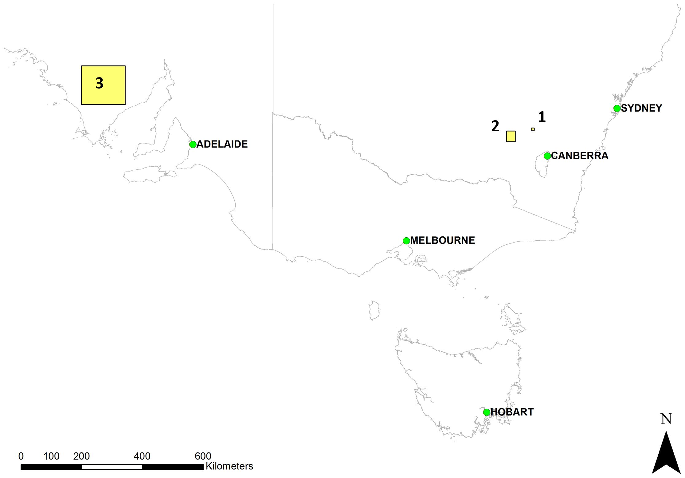
Figure 1. Locations of soil moisture sensor networks used in the study: (1) CSIRO Boorowa, (2) Muttama Creek Catchment, (3) Eyre Peninsula.

2.1.1 CSIRO Boorowa Agricultural Research Station

The 220 ha Boorowa Agricultural Research Station (BARS) is located 3 km south of Boorowa, NSW [34.4386°S, 148.7231°E]. The region has a temperate climate, receiving approximately 619 mm of annual rainfall, and features soils derived from Silurian volcanic materials. These soils are primarily classified as Yellow and Red Chromosols or Kurosols (20), depending on the presence of subsoil acidity. According to the World Reference Base for Soil Resources (21), these correspond to Luvisols, Lixisols, or Acrisols, respectively.

Thirty-three capacitance probes are installed across BARS (Figure 2), each 160 cm long (buried at 20 cm) and measuring at eight depths (30–170 cm) daily since September 2019. Probes measure relative permittivity, which is converted to volumetric soil moisture (θ) using factory calibration adjusted for temperature, followed by a 2-point site-specific rescaling (22). This scaling uses estimated drained upper limit (DUL) and lower limit (LL) values derived via pedotransfer functions (23), informed by soil texture, bulk density, carbon, and cation exchange capacity.

Rescaled soil moisture (Equation 1) is calculated as:

$\begin{array}{ll}{\theta }^S=\frac{DU{L}_{MM}-L{L}_{MM} }{DU{L}_{obs}-L{L}_{obs}} \times ({\theta }^F-DU{L}_{obs})+ DU{L}_{MM}& (1)\end{array}$

Here, ${\theta }^S$ is the rescaled soil moisture, ${\theta }^F$is the factory-calibrated moisture. $DU{L}_{MM}$ and $L{L}_{MM}$ correspond to the measured or modelled DUL and LL respectively, while $DU{L}_{obs}$ and $L{L}_{obs}$ correspond to the observed sensor upper and lower readings. The observed sensor limits are estimated using the 95th and 5th percentiles. PAW is computed as. ${\theta }^S-L{L}_{MM}$ While the 2-point scaling has assumptions—especially regarding DUL and LL correspondence—ongoing sensor data can refine these calibrations over time. Where feasible, measured DUL and LL improve reliability, though require more extensive fieldwork (24).

2.1.2 Muttama Creek Catchment

The Muttama Creek Catchment (MCC) spans 1,025 km² in the Murrumbidgee catchment of NSW, receiving 585–815 mm of annual rainfall. Land use is dominated by mixed cropping and grazing systems. Eight Sentek drill-and-drop probes (Figure 2), each with sensors at depths from 30 to 100 cm, were installed using a stratified sampling approach based on soil clay content (25), elevation, land use, and site access.

Sensor outputs were converted back to sensed frequency (SF) using the default Sentek calibration (26):

$\begin{array}{ll}SF=a*{\theta }_V^b+c& (2)\end{array}$

where a = 0.232, b = 0.41, and c = −0.02. 2-point scaling was then applied to SF using site-specific DUL and LL values estimated via Padarian (23) pedotransfer functions, as described above.

2.1.3 Eyre Peninsula

The Eyre Peninsula (EP) in South Australia covers ~170,000 km², with annual rainfall ranging from 250 mm (north) to 500 mm (south) and is characterized by diverse dryland cropping and grazing systems. Soils vary widely across the region, including calcareous soils, deep loams, sands, and red-brown earths.

A network of 43 capacitance probes (Figure 2) has been in place since 2016 and is publicly accessible through the National Soil Moisture Data Federation system (27). 2-point scaling was applied to raw probe data at each site using DUL and LL values, either measured directly or estimated via pedotransfer relationships based on co-located soil attribute data (e.g., texture, bulk density).

Figure 2

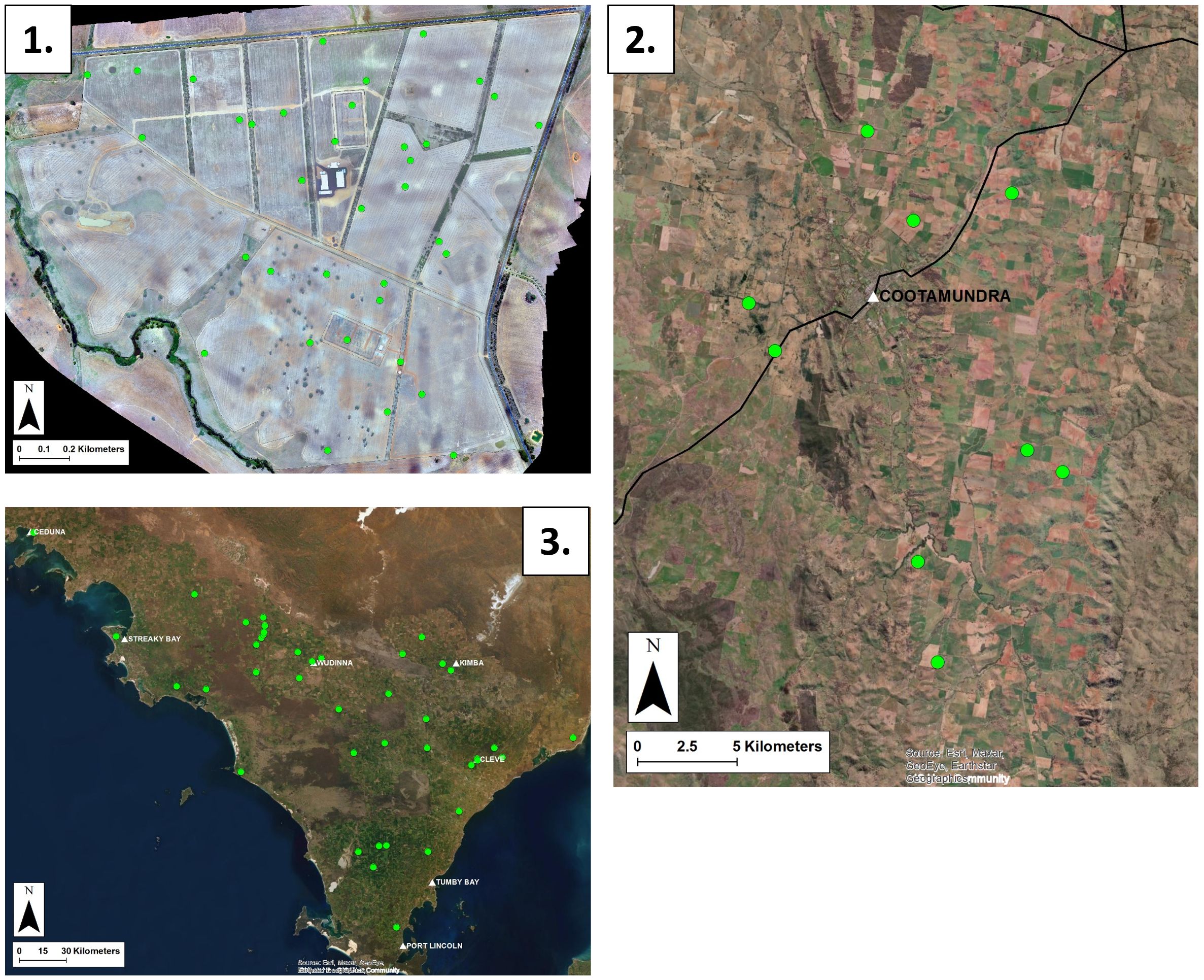
Figure 2. Distribution of soil moisture probes across the three study areas. (1) CSIRO Boorowa, (2) Muttama Creek Catchment, (3) Eyre Peninsula.

2.2 Description of soil water models

Four national-scale soil water balance models were assessed (Table 1), each differing in spatial resolution, depth support, model mechanics, and assimilation of satellite data.

Table 1

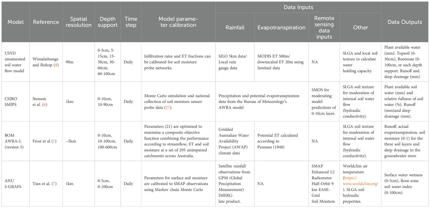
Table 1. Key attributes, inputs and outputs of the four considered models.

2.2.1 USYD model

Described by Wimalathunge and Bishop (8), the USYD model is a daily timestep, multi-layer unsaturated flow model with 90 m resolution, supporting application at continental scale using inputs from the Soil and Landscape Grid of Australia (28). The model simulates infiltration through five soil layers (0–100 cm) using DUL and LL values derived via Padarian (23) pedotransfer functions. Water moves freely between layers; excess beyond 100 cm is lost as deep drainage. Surface runoff occurs only when both top layers (0–15 cm) are saturated. Output is volumetric soil moisture in mm.

2.2.2 SMIPS model

SMIPS (6) is a 2-layer (0–10 cm, 10–90 cm) model operating at 1 km resolution. It produces daily PAW and percent full estimates. The upper layer is adjusted using SMOS satellite data (29) via a calibrated weighting scheme informed by comparisons with national soil moisture sensor networks (27). Vertical water flow between layers is governed by spatially varying parameters tied to soil texture.

2.2.3 AWRA-L model

AWRA-L (1) is a 0.05° (~5 km) resolution model operational since 2015. It simulates water fluxes through soil, groundwater, and surface stores using semi-distributed hydrological response units. Root-zone moisture is defined as the sum of two layers (0–10 cm and 10–100 cm) and expressed as percent saturation. Soil properties are drawn from ASRIS (30), with drainage and moisture dynamics calculated from daily water balance equations.

2.2.4 S-GRAFS model

S-GRAFS (7) combines a first-order Antecedent Precipitation Index (API) model with SMAP satellite soil moisture using four-dimensional variational data assimilation (4DVAR). Driven by GPM precipitation, it generates 1 km soil moisture estimates at both surface (5 cm) and root-zone (~1 m) depth. Root-zone moisture is derived using an exponential filter (SWI) and expressed as a percentage of saturation.

2.3 Post-processing of model outputs and sensor data

Despite similar conceptual underpinnings—partitioning rainfall into storage, runoff, evapotranspiration, and drainage—these models vary in implementation, including depth support, resolution, and units. SMIPS supports 0–90 cm; USYD and AWRA-L use 0–100 cm; S-GRAFS provides ‘root-zone’ estimates, assumed to correspond to 0–90 or 0–100 cm for harmonization. Output units vary between volumetric (mm of PAW) and percent saturation.

To enable comparison with sensor observations, all model outputs were standardized to a 0–90 cm depth and converted to PAW (mm). Sensor data at BARS and Muttama were similarly adjusted using DUL and LL estimates (23), with values aggregated across depths to 90 cm. PAW was calculated by subtracting LL from total water.

Model harmonization steps included:

● For SMIPS, outputs were already in PAW.

● For the USYD model, total water outputs were adjusted to PAW using predicted lower limit (LL) values (31), then scaled to 0–90 cm by multiplying by 0.9. This proportional adjustment assumes near-uniform water distribution across the profile and was adopted as a practical harmonization step to enable comparison across models with differing depth support. We acknowledge this is a simplification, and more refined scaling methods may be explored in future work.

● For AWRA-L and S-GRAFS, outputs in percent saturation were first converted to volumetric values using 2-point scaling (Equation 1) based on estimated DUL and LL. These were then scaled to 0–90 cm by multiplying by 0.9, with the same caveats acknowledged for the USYD model regarding uniform moisture distribution. Finally, the adjusted values were converted to PAW

Calibration windows from 2018–2022 ensured inclusion of both dry (pre-March 2020) and wet (post-2020) periods. Model outputs were spatially intersected with soil probe locations for direct comparison, ensuring harmonized resolution, depth, and units prior to model averaging analysis.

2.4 Model averaging methodology

2.4.1 Probe-level model averaging

With all model outputs and sensor data harmonized to a common 0–90 cm depth and in units of plant available water (PAW, mm), we first conducted a probe-level comparison across each region for the 2021 calendar year. This involved evaluating how each individual model corresponded with soil moisture sensor data prior to applying two model averaging approaches:

● Equal Weighting (EW): A simple unweighted mean of the four models, assigning each a weight of 0.25.

● Granger–Ramanathan Averaging (GRA): A more sophisticated method that fits a linear regression between the sensor data (${\theta }^S$) and the model outputs $X_{USYD},X_{AWRA},X_{SMIPS},X_{SGRAFS}$, allowing each model’s contribution to vary according to its covariance with observed values. The fitted model takes the form:

The fitted model (Equation 3) takes the form:

$\begin{array}{ll}\begin{array}{c}{\theta }^S= W_0+(W_{USYD} \times X_{USYD} )\\ + (W_{AWRA} \times X_{AWRA} )+ (W_{SMIPS} \times X_{SMIPS} )\\ + (W_{SGRAFS} \times X_{SGRAFS} )\end{array}& (3)\end{array}$

Here, W₀ represents the intercept or bias correction term, and the other W_.. variables are fitted OLS parameters, for each of the model variables (outputs from each of the different water balance models). Unlike EW or variance-weighted approaches (e.g. Bates-Granger), GRA inherently adjusts for systematic biases and exploits correlations in model errors, which is particularly relevant for models that share error structure but differ in magnitude or offset.

2.4.2 Spatial model averaging approaches

While probe-level averaging evaluates model skill at specific points, practical use cases demand spatially explicit maps. Given that the underlying models produce gridded outputs, spatial model averaging enables generation of composite maps, but GRA poses challenges due to the site-specific nature of its coefficients.

We explored four strategies for spatializing GRA parameters using data from the BARS site:

1. Temporally Fixed GRA (TF): All probe data combined into a single dataset; one set of GRA coefficients fitted across the full 2021 time series.

2. Temporally Varying GRA (TC): A rolling 25-day window used to fit new GRA coefficients each day, aiming to capture temporal changes in soil wetting and drying dynamics. The choice of a 25-day rolling window for dynamic GRA was intended to approximate a near-monthly scale while preserving enough data points for robust regression fitting.

3. Temporally Fixed GRA with Covariates (TFC): Same as TF, but with additional spatial covariates (topographic, climatic, and gamma radiometric data) drawn from TERN’s 30 m resolution covariate stack (32).

4. Temporally Varying GRA with Covariates (TCC): Same as TC but incorporating the same spatial covariates, aiming to improve spatial prediction accuracy by accounting for environmental heterogeneity.

All spatial model outputs were harmonized to 90 m resolution (matching the USYD model) using bilinear interpolation. For this study, we focus on two key dates—1 April and 1 July 2021—selected to reflect pre-planting and in-crop management phases of the winter cropping cycle.

2.5 Evaluation metrics

Model and model-averaged predictions were assessed against soil moisture probe observations using two metrics:

● Pearson Correlation (r): Captures the strength and shape of the relationship (wetting and drying dynamics) between model output and sensor data.

● Lin’s Concordance Correlation Coefficient (ρ_c): Evaluates both correlation and agreement, providing a measure of prediction skill by quantifying deviation from the 1:1 line.

These metrics were applied to both probe-level and spatial predictions (at BARS only), enabling comparison across individual models, EW averaging, and the different GRA approaches.

3 Results and discussion

3.1 Probe-level evaluations

To assess model performance at point scale, we examined soil moisture traces from the 2021 calendar year, comparing in situ sensor data with outputs from individual soil water balance (SWB) models and two model averaging approaches: equal weighting (EW) and Granger–Ramanathan (GRA). Figure 3 presents representative examples from each study area.

Figure 3

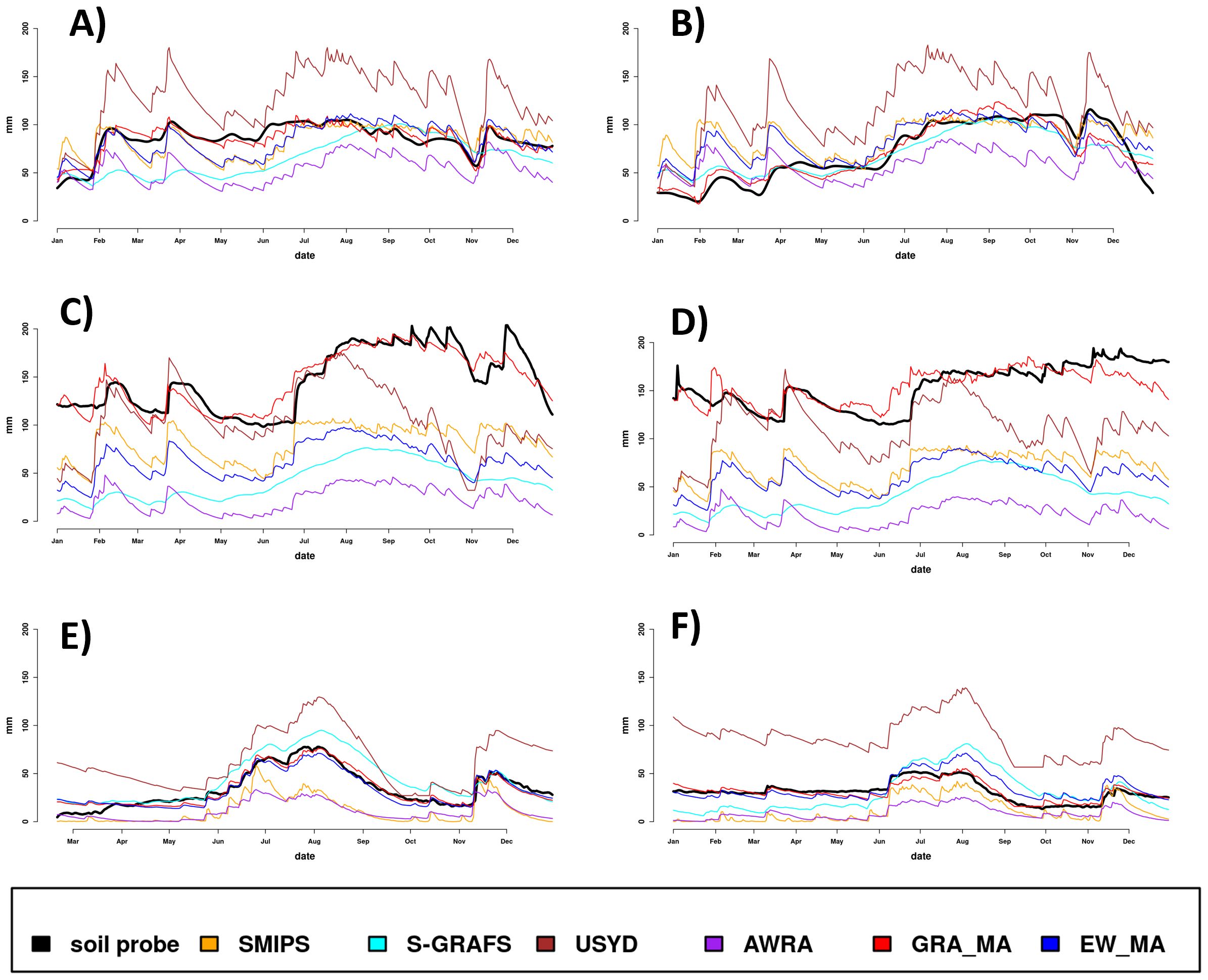
Figure 3. Soil moisture traces from selected probes during the 2021 calendar year. (A, B) BARS probes #127 and #179; (C, D) Muttama probes #X1 and #X7; (E, F) Eyre Peninsula probes #20610 and #40112. Black = probe data; Orange = SMIPS; Cyan = S-GRAFS; Brown = USYD; Purple = AWRA-L; Blue = EW average; Red = GRA average.

3.1.1 BARS

At the Boorowa Agricultural Research Station (BARS), all SWB models demonstrated a reasonable ability to track observed soil moisture dynamics (Figures 3A, B). Table 2 summarizes evaluation metrics across the 33 probes. While correlation values were generally high for all models, there was no consistent standout across all locations. On a probe-by-probe basis, the best-performing model varied.

Table 2

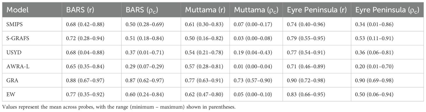
Table 2. Summary of correlation and concordance between soil moisture sensor data and soil water balance (SWB) model outputs and model averages across all sites.

However, concordance results revealed systematic bias in several models—most notably USYD and AWRA-L—which impacted overall agreement with observed data. Both model averaging methods mitigated these discrepancies to some extent. EW averaging improved general fit, but GRA model averaging was clearly superior, achieving near-perfect alignment with sensor traces in many instances.

3.1.2 Muttama Creek Catchment

Model performance at the Muttama Creek Catchment was broadly like BARS, though average correlations were slightly lower (Figures 3C, D). USYD tended to show the highest concordance among individual models, but again, performance varied across probes. The relatively more complex terrain at Muttama may have contributed to this variability.

EW averaging provided comparable correlation to individual models but underperformed in concordance, largely due to its inability to correct for model-specific biases. In contrast, GRA averaging substantially improved both metrics, again highlighting its effectiveness in synthesizing diverse model outputs.

3.1.3 Eyre Peninsula

Despite its distinct soils and climate, model behavior at Eyre Peninsula was consistent with that observed at the other sites (Figures 3E, F). All individual models performed reasonably well, although none emerged as consistently superior. As with BARS and Muttama, model performance was probe dependent.

GRA averaging once again delivered the strongest and most consistent performance across metrics (Table 2), reinforcing its robustness and adaptability across varying landscapes. These findings support model averaging—particularly GRA—as a practical strategy for integrating diverse SWB model outputs at the probe scale.

3.2 Spatialization of GRA model averaging summary of models and their parameters

Two sets of smoothed density plots were generated to visualize the performance of the four spatial model configurations—TF, TFC, TC, and TCC—across the 33 BARS soil moisture probe locations, using Pearson correlation and Lin’s concordance correlation coefficient (CCC) as evaluation metrics (Figure 4). For reference, the density plots also include results summarized in previous section from the probe-level analysis using EW and GRA averaging, which serve as useful benchmarks for comparison. Each plot overlays kernel density curves for six model configurations, enabling direct visual comparison of how correlation and concordance values are distributed across all probes. Narrow, peaked curves near 1.0 indicate consistently strong performance, while broader or flatter curves suggest greater variability among sites.

Figure 4

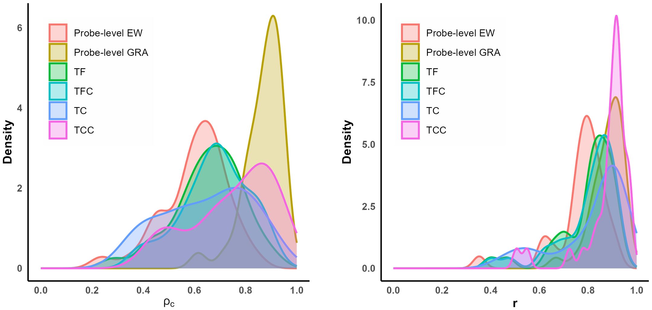
Figure 4. Smoothed density plots of Pearson correlation (r) and Lin’s concordance correlation coefficient (ρ_c) illustrating model performance across 33 BARS soil moisture probe locations. The plots compare four spatial model configurations—Temporally Fixed (TF), Temporally Fixed with Covariates (TFC), Temporally Varying (TC), and Temporally Varying with Covariates (TCC)—against probe-level model averaging results using Equal Weighting (EW) and Granger–Ramanathan (GRA).

The correlation plots show clear distinctions between the EW and GRA outcomes at the probe level. All four spatial models display peaks around 0.9, suggesting they capture the temporal patterns of soil moisture traces reasonably well. Among the spatial approaches, the TC and TCC models—those incorporating temporally varying GRA coefficients—demonstrate the strongest performance, with TCC (which includes both temporal structure and environmental covariates) yielding the highest overall scores.

In the concordance plots, however, the TC and TCC curves are noticeably flatter than the probe-level GRA model, indicating a loss of site-specific precision when probe data are aggregated to fit global GRA coefficients. Despite this, TCC still outperforms TC, visually reinforcing the benefit of incorporating spatial covariates alongside temporal structure. The TC model, while lacking covariate inputs, still performs favorably, highlighting the value of temporal adaptiveness alone.

The TF and TFC models, which use static coefficients, show broader concordance distributions, pointing to less consistent agreement with probe measurements. Although their correlation densities remain relatively high—indicating they capture general wetting and drying trends—their lower concordance values suggest systematic biases or mismatches in magnitude.

Overall, these dual-density plots provide a nuanced view of model performance. Incorporating temporal variation in GRA coefficients consistently enhances predictions. When environmental covariates are added, further improvements are achieved, likely because these covariates help characterize the local conditions at sensor locations. In contrast, incorporating covariates alone (as in TFC) without temporal variation offers limited benefit, indicating an interaction effect between spatial and temporal factors in model performance. The parameter coefficients for both TF and TFC GRA models are provided in the Supplementary Material.

3.3 Spatialization of GRA model averaging

Spatial implementation of model averaging is relatively straightforward for both EW and GRA approaches. For EW, provided that all input maps have been harmonized in terms of depth support, data units, and spatial resolution, model averaging is simply the arithmetic mean—i.e., each SWB model output receives an equal weight of 0.25. Figure 5 shows individual SWB model outputs for the selected dates of 1st April and 1st July 2021, while Figure 6 presents the corresponding EW model averaging outputs. Notably, S-GRAFS and AWRA-L produce relatively less spatial variation compared to the USYD and SMIPS models, likely due to differences in spatial resolution and input data (e.g. SMAP satellite inputs in S-GRAFS). As expected, EW model averaging generates maps that broadly reflect the central tendencies of the contributing models.

Figure 5

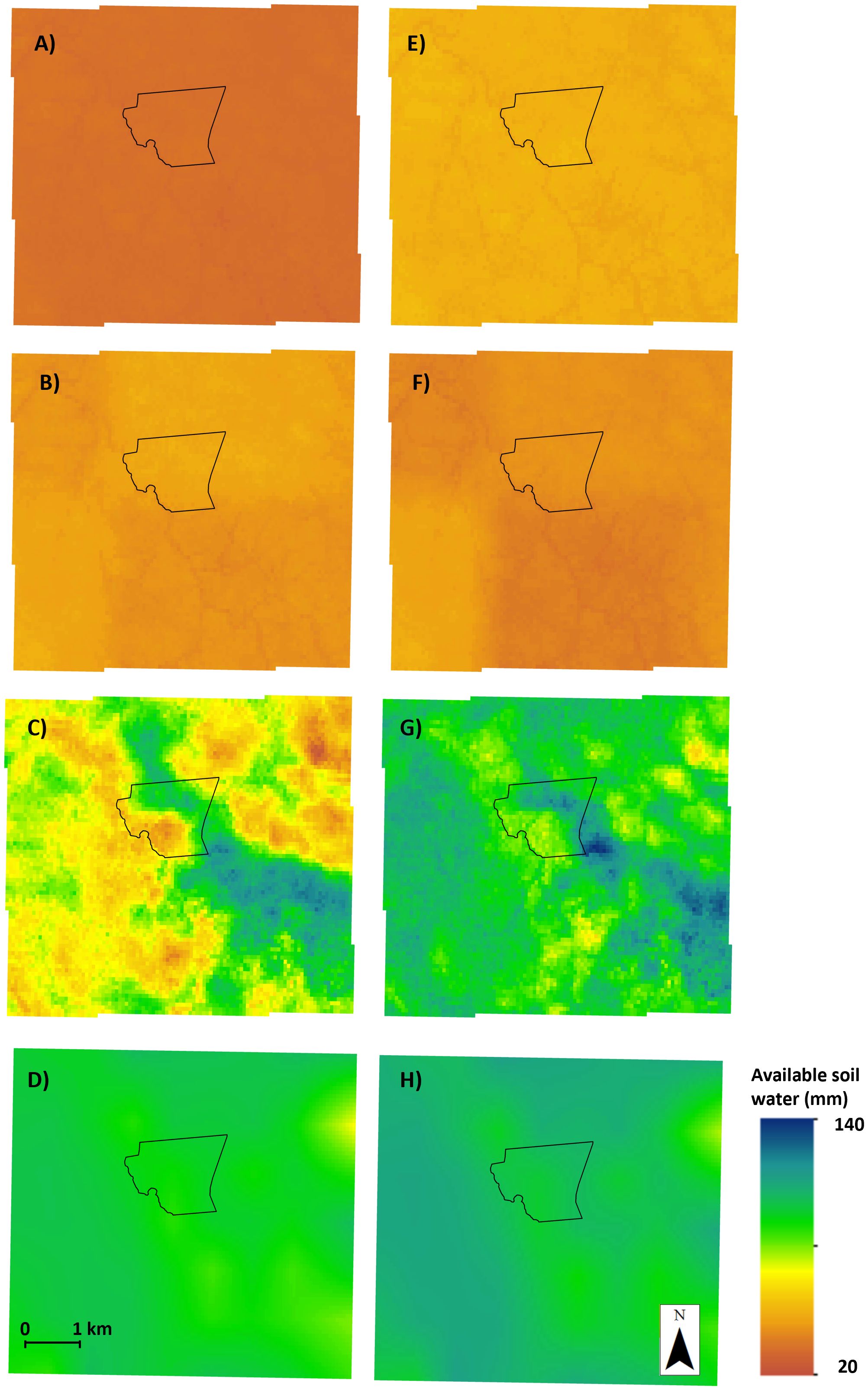
Figure 5. Soil moisture mapping outputs from each of the SWB models for the BARS region on 1st April and 1st July 2021. (A–D) April maps for S-GRAFS, AWRA-L, USYD, and SMIPS, respectively; (E–H) corresponding July maps. All maps are harmonized to PAW (mm) at 0–90 cm depth and 90 m resolution.

Figure 6

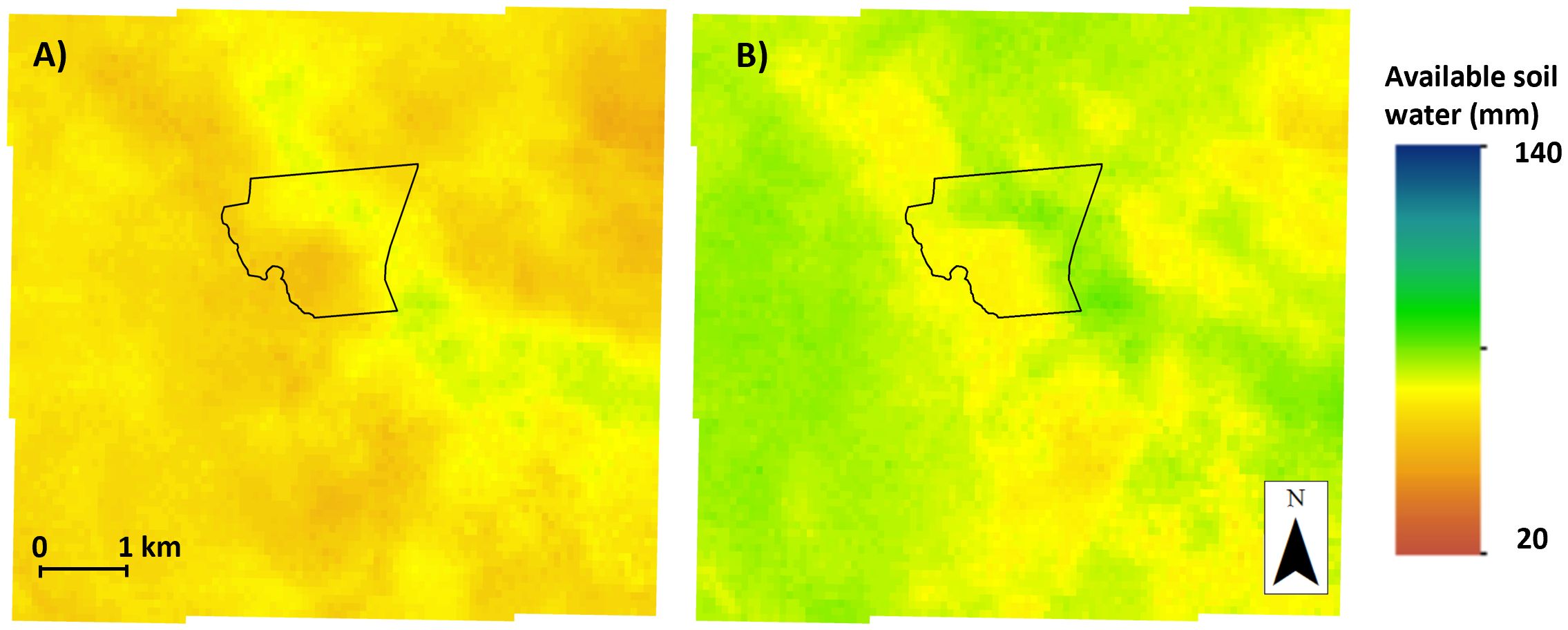
Figure 6. Soil moisture maps from equal-weight model averaging on (A) 1st April and (B) 1st July 2021, using harmonized SWB model outputs.

Figure 7 presents the mapping outputs from the four GRA spatial model configurations (TF, TFC, TC, and TCC) for the same two dates. In the absence of covariates (TF and TC; Figures 7A, C), the resulting spatial patterns are generally comparable to the EW maps. The TC model, which uses temporally varying GRA coefficients, displays greater spatial detail—likely reflecting its more date-specific parameterization. While this may better reflect true spatial soil moisture variability, definitive conclusions would require independent validation data.

Figure 7

Figure 7. Soil moisture mapping outputs using GRA model averaging configurations: (A–D) show TF, TFC, TC, and TCC models for 1st April; (E–H) show the same configurations for 1st July 2021. All maps are shown at 90 m resolution and scaled to PAW (mm, 0–90 cm).

The inclusion of environmental covariates (TFC and TCC; Figures 7B, D) has a much more pronounced effect. When model coefficients trained at probe locations are extrapolated using covariates, large regions of the mapping extent exhibit unusually low PAW values. This pattern suggests that the environmental characteristics at probe locations are not representative of the broader landscape, leading to poor generalization. The issue is most apparent in the TCC model, where the daily re-fitting of GRA coefficients compounds the mismatch between local training data and spatial covariate coverage.

These results highlight an important nuance: although covariates improved model performance at the probe level (as seen in earlier evaluations), they did not translate well to spatial prediction. This likely reflects a combination of factors, including the limited number of probe locations, the relatively small spatial extent of BARS, and the risk of overfitting to locally specific conditions.

While incorporating environmental covariates can help capture spatial gradients, their effectiveness is limited when sensor networks are sparse or spatially clustered. In such cases, alternative spatialization strategies may offer greater robustness. One promising direction is to aggregate the landscape into hydrological response units, soil functional classes, or other stratified land units. Within these strata, probe data can be used to define class-specific temporal patterns, enabling regionally generalized model averaging. This more structured approach to scaling may be better suited to operational mapping and warrants further exploration—a concept we expand upon in the subsequent discussion.

4 General discussion

This investigation aimed to evaluate the efficacy of relatively simple model averaging approaches for combining national-scale operational soil water balance (SWB) models into a unified estimate. The motivation was to reduce decision-making complexity for farm operators, who are otherwise left to reconcile potentially conflicting outputs from individual models. As demonstrated, the four SWB models assessed—SMIPS, AWRA-L, S-GRAFS, and USYD—can produce markedly different estimates of plant-available water (PAW) for the same location and day. These discrepancies arise from differences in model structure, resolution, inputs, and inherent biases.

Our probe-level evaluations across three diverse regions revealed no single model consistently outperformed the others. Instead, model performance varied unpredictably by location, underscoring the challenge for users seeking reliable guidance from any one model. In this context, model averaging emerges as a practical strategy that can consolidate strengths and mitigate weaknesses without necessitating the development of an entirely new modelling framework.

Equal-weight (EW) model averaging, though simple, does not account for model-specific biases or relative performance. At the probe level, EW averaging sometimes performed worse—particularly in terms of concordance—than the best individual models, as it lacks a mechanism for bias correction. Nevertheless, when applied spatially, EW averaging produced reasonable results and may serve as a low-risk, computationally efficient default when no clear model preference exists. Given the unpredictable model performance across probe locations, EW averaging represents a viable and easily implemented compromise.

In contrast, Granger–Ramanathan (GRA) model averaging offers a more robust and statistically grounded alternative. At the probe scale, GRA outperformed individual models and EW averaging, strongly supporting the first hypothesis of this investigation. GRA’s key advantage lies in its ability to correct for bias and exploit covariance among model errors, allowing it to generate predictions that more closely match sensor observations.

Soil moisture sensor networks play a critical role in enabling GRA model averaging by providing the observational data required to calibrate model weights. However, a key challenge emerged in translating probe-level GRA insights into spatially continuous maps. The second hypothesis—that spatially scaled GRA coefficients would produce superior PAW maps—was not supported. This limitation is primarily due to the sparse and clustered nature of most probe networks, which limits the geographic representativeness of GRA parameters derived from them.

We explored this issue through a case study at BARS farm, applying several GRA spatialization strategies, including temporally fixed and varying coefficients, with and without the inclusion of environmental covariates. While temporally varying models (TC and TCC) provided improved probe-level performance, the inclusion of covariates introduced substantial spatial artefacts when extrapolated across the mapping domain. This was most evident in the TCC model, where exaggerated low values appeared in regions far from sensor locations. These artefacts likely arise from a mismatch between the environmental feature space of the probe locations and that of the broader landscape, leading to poor generalization of model parameters.

Although environmental covariates provide valuable context for spatial prediction, their utility is limited when probe networks are spatially clustered and fail to represent the full variability of the covariate feature space. An alternative strategy is to stratify the landscape into hydrological response units (HRUs) or soil functional classes, which can reduce sensitivity to localized calibration and improve the generalizability of model averaging approaches. HRUs are typically delineated using combinations of soil type, slope, land cover, and sometimes geology, and are widely employed in hydrological modelling frameworks such as SWAT (3). In large-scale applications, such as across the contiguous United States (CONUS), watershed-based units like the HUC8 subbasins have been used effectively to support spatially contextualized model training and reduce the risk of spurious predictions (33). These subbasins provide natural boundaries for defining the extent of model domains and retrieving relevant soil observations. Similar stratification approaches could be adopted in our study area using data from the TERN 30 m or 90 m environmental covariate stacks (32) to identify soil-hydrologically homogeneous regions based on variables such as slope, soil texture, soil thickness, and climatic regime. This concept is analogous to the work of McKenzie and Ryan (34), who defined functional soil domains by clustering landscapes based on pedogenic and environmental similarity. Applying such logic specifically to hydrological behavior offers a feasible and testable pathway to improve the spatial implementation of model averaging beyond point-based calibration.

Future work should also explore technical aspects of model harmonization. One of the challenges in multi-model integration is the differing spatial resolutions, measurement units, and depth support of the input models. While this study implemented a harmonization strategy across all four SWB models, there is clear scope for improving the scaling and alignment procedures—particularly spatial scaling.

There is also room for optimization in the temporal dimension of GRA model fitting. Our analysis used a rolling 25-day window at daily resolution. While this approach improved performance relative to year-long aggregates, shorter modelling windows may propagate noise and parameter instability. Future investigations should consider broader temporal intervals—weekly, monthly, or tied to agronomic events such as planting or fertilization—to balance flexibility with robustness and reduce cumulative error propagation.

Finally, alternative model combination strategies such as triple or quadruple collocation may provide promising avenues. These methods allow for the estimation of model errors without requiring ground observations and have been successfully applied in meteorological and remote sensing contexts (35–37). Once error estimates are derived, weighted merging similar to GRA can be applied. Importantly, current applications of collocation techniques rely on ground truth data solely for validation, but future work could investigate their integration into the model averaging process itself. Such innovations could ultimately support more generalizable and spatially robust soil moisture mapping systems—potentially addressing the second hypothesis under a more suitable methodological framework.

5 Conclusion

This study provides new insight into how model averaging—particularly the Granger–Ramanathan (GRA) approach—can be applied to improve both point-scale and spatial estimates of soil moisture. The research makes three key contributions. First, it demonstrates that GRA model averaging significantly improves agreement between modelled and observed plant-available water (PAW) at the probe level, outperforming both individual models and equal-weighted ensembles across diverse environments. Second, it introduces and evaluates a temporally dynamic implementation of GRA, enabling model weights to adapt to changing seasonal and soil moisture conditions—an innovation not previously applied in soil moisture modelling. Third, the study systematically tests spatial scaling strategies for GRA coefficients, including the use of environmental covariates, and highlights both the opportunities and pitfalls of extrapolating fitted weights beyond sensor network domains.

These findings have practical implications for real-time soil water monitoring and decision-support systems. By leveraging data from existing national-scale SWB models and in situ networks, the proposed approach enables a more robust and flexible integration framework without the need to develop entirely new mechanistic models. However, the results also underscore the challenges of spatial generalization in data-sparse landscapes. Incorporating temporally dynamic weights improves prediction accuracy locally, but spatial extrapolation remains sensitive to the representativeness of training data and covariate selection.

Future work should focus on developing more stable spatialization frameworks, such as stratifying landscapes by hydrological or functional soil units, and further exploring hybrid or error-based merging methods (e.g. triple collocation) that do not rely exclusively on in situ observations. Advancing these strategies will be critical for delivering scalable, operational soil moisture products that support precision agriculture, drought monitoring, and environmental management.

Data availability statement

Publicly available datasets were analyzed in this study. Real time and historical soil moisture data from CSIRO Boorowa Farm may be accessed through the ERATOS platform dashboard (https://senaps.eratos.com/#/app/group/detail/dsapi-outgoing-fresh-dealer). An account will first need to be established with the ERATOS team to access those data. All other data that support this study will be made available by the authors, without undue reservation.

Author contributions

BM: Formal Analysis, Resources, Data curation, Validation, Conceptualization, Methodology, Supervision, Investigation, Writing – original draft, Writing – review & editing. RS: Data curation, Methodology, Resources, Writing – review & editing, Writing – original draft. ST: Validation, Resources, Writing – review & editing, Data curation, Investigation. TB: Methodology, Writing – review & editing, Investigation, Conceptualization, Funding acquisition, Resources. YY: Investigation, Writing – review & editing, Resources.

Funding

The author(s) declare financial support was received for the research and/or publication of this article. The authors declare that this study received funding from the Grains Research and Development Corporation project SoilWaterNow: Soil water nowcasting for the grains industry (UOS2002-001RTX). The funder was not involved in the study design, collection, analysis, interpretation of data, the writing of this article or the decision to submit it for publication.

Conflict of interest

The authors declare that the research was conducted in the absence of any commercial or financial relationships that could be construed as a potential conflict of interest.

The author(s) declared that they were an editorial board member of Frontiers, at the time of submission. This had no impact on the peer review process and the final decision.

Generative AI statement

The author(s) declare that no Generative AI was used in the creation of this manuscript.

Any alternative text (alt text) provided alongside figures in this article has been generated by Frontiers with the support of artificial intelligence and reasonable efforts have been made to ensure accuracy, including review by the authors wherever possible. If you identify any issues, please contact us.

Publisher’s note

All claims expressed in this article are solely those of the authors and do not necessarily represent those of their affiliated organizations, or those of the publisher, the editors and the reviewers. Any product that may be evaluated in this article, or claim that may be made by its manufacturer, is not guaranteed or endorsed by the publisher.

Supplementary material

The Supplementary Material for this article can be found online at: https://www.frontiersin.org/articles/10.3389/fsoil.2025.1629686/full#supplementary-material

References

1. Frost AJ, Ramchurn A, and Smith A. The bureau’s operational AWRA landscape (AWRA-L) model. Melbourne, Australia: Australian Bureau of Meteorology Technical Report (2016).

Google Scholar

2. Hillel D. Fundamentals of soil physics. New York, New York: Elsevier Inc (1980).

Google Scholar

3. Gassman PW, Reyes MR, Green CH, and Arnold JG. The soil and water assessment tool: historical development, applications, and future research directions. Trans ASABE. (2007) 50:1211–50. doi: 10.13031/2013.23637

Crossref Full Text | Google Scholar

4. Keating BA, Carberry PS, Hammer GL, Probert ME, Robertson MJ, Holzworth D, et al. An overview of APSIM, a model designed for farming systems simulation. Eur J Agron. (2003) 18:267–88. doi: 10.1016/S1161-0301(02)00108-9

Crossref Full Text | Google Scholar

5. Jones JW, Hoogenboom G, Porter CH, Boote KJ, Batchelor WD, Hunt LA, et al. The DSSAT cropping system model. Eur J Agron. (2003) 18:235–65. doi: 10.1016/S1161-0301(02)00107-7

Crossref Full Text | Google Scholar

6. Stenson M, Searle R, Malone BP, Sommer A, Renzullo LJ, and Di H. Australia wide daily volumetric soil moisture estimates. Version 1.0 [Dataset]. Canberra: Terrestrial Ecosystem Research Network (2021). doi: 10.25901/b020-nm39

Crossref Full Text | Google Scholar

7. Tian S, Renzullo LJ, and Cai D. Satellite-driven 10km global root-zone soil moisture analysis for drought monitoring [Dataset]. Canberra, Australia: Zenodo (2023). doi: 10.5281/zenodo.7553987

Crossref Full Text | Google Scholar

8. Wimalathunge NS and Bishop TFA. A space-time observation system for soil moisture in agricultural landscapes. Geoderma. (2019) 344:1–13. doi: 10.1016/j.geoderma.2019.03.002

Crossref Full Text | Google Scholar

9. Diks CGH and Vrugt JA. Comparison of point forecast accuracy of model averaging methods in hydrologic applications. Stochastic Environ Res Risk Assess. (2010) 24:809–20. doi: 10.1007/s00477-010-0378-z

Crossref Full Text | Google Scholar

10. Raftery AE, Gneiting T, Balabdaoui F, and Polakowski M. Using bayesian model averaging to calibrate forecast ensembles. Monthly Weather Rev. (2005) 133:1155–74. doi: 10.1175/MWR2906.1

Crossref Full Text | Google Scholar

11. Rojas R, Feyen L, and Dassargues A. Conceptual model uncertainty in groundwater modeling: Combining generalized likelihood uncertainty estimation and Bayesian model averaging. . Water Resour Res. (2008) 44:1–16. doi: 10.1029/2008WR006908

Crossref Full Text | Google Scholar

12. Malone BP, Luo Z, He D, Viscarra Rossel RA, and Wang E. Bioclimatic variables as important spatial predictors of soil hydraulic properties across Australia’s agricultural region. Geoderma Regional. (2020) 23:e00344. doi: 10.1016/j.geodrs.2020.e00344

Crossref Full Text | Google Scholar

13. O’Rourke SM, Stockmann U, Holden NM, McBratney AB, and Minasny B. An assessment of model averaging to improve predictive power of portab le vis-NIR and XRF for the determination of agronomic soil properties. Geoderma. (2016) 279:31–44. doi: 10.1016/j.geoderma.2016.05.005

Crossref Full Text | Google Scholar

14. Bates JM and Granger CWJ. The combination of forecasts. JSTOR. (1969) 20:451–68. doi: 10.2307/3008764

Crossref Full Text | Google Scholar

15. Heuvelink GBM and Bierkens MFP. Combining soil maps with interpolations from point observations to predict quantitative soil properties. Geoderma. (1992) 55:1–15. doi: 10.1016/0016-7061(92)90002-O

Crossref Full Text | Google Scholar

16. Hoeting JA, Madigan D, Raftery AE, and Volinsky CT. Bayesian model averaging: a tutorial (with comments by M George rejoinder by authors. Stat Sci. (1999) 14:382–417. doi: 10.1214/ss/1009212519

Crossref Full Text | Google Scholar

17. Buckland ST, Burnham KP, and Augustin NH. Model selection: an integral part of inference. Biometrics. (1997) 53:603–18. doi: 10.2307/2533961

Crossref Full Text | Google Scholar

18. Hansen BE. Least squares model averaging. Econometrica. (2007) 75:1175–89. doi: 10.1111/j.1468-0262.2007.00785.x

Crossref Full Text | Google Scholar

19. Granger CWJ and Ramanathan R. Improved methods of combining forecasts. J Forecasting. (1984) 3:197–204. doi: 10.1002/for.3980030207

Crossref Full Text | Google Scholar

20. Isbell R and National Committee on Soil and Terrain. The Australian soil classification. 3rd Edition. Melbourne, Australia: CSIRO publishing (2021).

Google Scholar

21. IUSS Working Group WRB. World Reference Base for Soil Resources. International soil classification system for naming soils and creating legends for soil maps. 4th edition. Vienna, Austria: International Union of Soil Sciences (IUSS (2022).

Google Scholar

22. Gasch CK, Brown DJ, Brooks ES, Yourek M, Poggio M, Cobos DR, et al. A pragmatic, automated approach for retroactive calibration of soil moisture sensors using a two-step, soil-specific correction. Comput Electron Agric. (2017) 137:29–40. doi: 10.1016/j.compag.2017.03.018

Crossref Full Text | Google Scholar

23. Padarian J. Provision of soil information for biophysical modelling. Masters thesis. Sydney, Australia: Department of Agriculture; Environment, The University of Sydney (2014).

Google Scholar

24. McKenzie NJ, Coughlan K, and Cresswell H. Soil physical measurement and interpretation for land evaluation. Collingwood: CSIRO Pubishing (2002).

Google Scholar

25. Orton TG, Pringle MJ, and Bishop TFA. A one-step approach for modelling and mapping soil properties based on profile data sampled over varying depth intervals. Geoderma. (2016) 262:174–86. doi: 10.1016/j.geoderma.2015.08.013

Crossref Full Text | Google Scholar

26. Dalton M, Buss P, Treijs A, and Portmann M. (2015)., in: Correction for temperature variation in Sentek Drill & Drop soil water capacitance probes, Irrigation Australia Limited Regional Conference, Penrith Panthers, Western Sydney, May 26-28, 2015. (Brisbane, Australia: Irrigation Australia Limited)

Google Scholar

27. Stenson M, Sommer A, Searle R, and Freebairn D. (2018). “Federating and harmonising disparate soil moisture data sources” in: 13th International Conference on Hydroinformatics, London, UK: International Water Association. pp. 2019–2027.

Google Scholar

28. Malone BP, Searle R, Stenson M, McJannet D, Zund P, Román Dobarco M, et al. Update and expansion of the soil and landscape grid of Australia. Geoderma. (2025) 455:117226. doi: 10.1016/j.geoderma.2025.117226

Crossref Full Text | Google Scholar

29. Kerr YH, Waldteufel P, Richaume P, Wigneron JP, Ferrazzoli P, Mahmoodi A, et al. The SMOS soil moisture retrieval algorithm. IEEE Trans Geosci Remote Sens. (2012) 50:1384–403. doi: 10.1109/TGRS.2012.2184548

Crossref Full Text | Google Scholar

30. Johnston RM, Barry SJ, Bleys E, Bui EN, Moran CJ, Simon DAP, et al. ASRIS: the database. Soil Res. (2003) 41:1021–36. doi: 10.1071/SR02033

Crossref Full Text | Google Scholar

31. Searle R and Malone B. 30m resolution soil water parameter modelling. Brisbane: CSIRO (2021) p. EP2022–3598. doi: 10.25919/j31c-rj75

Crossref Full Text | Google Scholar

32. Searle R, Malone B, Wilford J, Austin J, Ware C, Webb M, et al. TERN digital soil mapping raster covariate stacks. v2. Brisbane, Australia: CSIRO (2022). doi: 10.25919/jr32-yq58n

Crossref Full Text | Google Scholar

33. Xu C, Huang J, Hartemink AE, and Chaney NW. Pruned hierarchical Random Forest framework for digital soil mapping: Evaluation using NEON soil properties. Geoderma. (2025) 459:117392. doi: 10.1016/j.geoderma.2025.117392

Crossref Full Text | Google Scholar

34. McKenzie NJ and Ryan PJ. Spatial prediction of soil properties using environmental correlation. Geoderma. (1999) 89:67–94. doi: 10.1016/S0016-7061(98)00137-2

Crossref Full Text | Google Scholar

35. Stoffelen A. Toward the true near-surface wind speed: Error modeling and calibration using triple collocation. J Geophysical Research: Oceans. (1998) 103:7755–66. doi: 10.1029/97JC03180

Crossref Full Text | Google Scholar

36. Yilmaz MT, Crow WT, Anderson MC, and Hain C. An objective methodology for merging satellite- and model-based soil moisture products. Water Resour Res. (2012) 48:1–15. doi: 10.1029/2011WR011682

Crossref Full Text | Google Scholar

37. Fascetti F, Pierdicca N, Pulvirenti L, and Crapolicchio R. SMOS, ASCAT, SMAP and ERA soil moisture comparison through the triple and quadruple collocation technique, Proc. SPIE 10003. In: SAR image analysis, modeling, and techniques XVI (Bellingham, Washington USA: SPIE) (2016). p. 100030H.

Google Scholar