Variations in maximum freezing depth in Northeast China from 1975 to 2024 using a machine learning model

A freezing depth prediction model was constructed using machine learning, incorporating comprehensive data from ground meteorological monitoring stations and remote sensing reanalysis data. The maximum freezing depth (MFD) of seasonally frozen ground (SFG) in Northeast China was systematically analyzed from 1975 to 2024. The simulation results from the machine learning model (MLM) indicated that the MFD of SFG in Northeast China displayed a decreasing trend over the past 50 years, with an average rate of change of -8.54 cm per decade. The average maximum freezing depths (AMFDs) in Northeast China for each decade were: 136.71 cm (1975−1984), 131.96 cm (1985−1994), 123.07 cm (1995−2004), 110.82 cm (2005−2014), and 104.58 cm (2015−2024). The area occupied by each AMFD interval in Northeast China over the past 50 years increased in regions with freezing depths <160 cm. The area with freezing depths >160 cm displayed a decreasing trend. The results not only reveal the impact of climate change on freezing depths, but also provide a scientific basis for environmental management and ecological protection in frozen ground areas. Changes in freezing depth directly affect many sectors such as agriculture, construction, and transportation, making accurate prediction essential for developing climate adaptation strategies. Considering the lack of data regarding the MFD of SFG in Northeast China for the past 50 years, the MLM provided an effective method for predicting changes in MFD using meteorological data and remote sensing reanalysis data.

1 Introduction

Under the backdrop of continuous global warming, the freezing state and extent of seasonally frozen ground (SFG) have changed (1). Due to its unique geographical location and climatic conditions, Northeast China experiences long and harsh winters, resulting in the widespread distribution of permafrost and SFG. The depth of freezing in SFG substantially influences regional infrastructure development and agroecological systems (2, 3). In infrastructure construction activities, the freezing depth directly affects the magnitude of frost heave (4). Frost heave has a huge impact on the stability of engineering structures (5). The frost heave effect causes the foundations of a structure to lift or undergo lateral displacement, which will further weaken its bearing performance (6–8). The freezing depth influences the distribution of soil moisture, which subsequently impacts the absorption of water and nutrients by agricultural crops. Changes in freezing depths and freeze-thaw processes can damage soil structure (9), affect soil aeration and drainage, and may cause damage to agricultural facilities such as greenhouses and irrigation systems (10). With climate change, the variation in the freezing depth of SFG poses new challenges to the adaptability and sustainability of infrastructure construction and agricultural production in Northeast China. Therefore, exploring the variation of the maximum freezing depth (MFD) has very important practical implications. Furthermore, the scarcity of meteorological stations in remote and cold regions makes it prohibitively expensive to conduct continuous monitoring activities to obtain observational data. Consequently, adopting feasible new approaches to predict long-term changes in freezing depth represents an effective solution to this problem (11).

SFG is a critical component of the cryosphere, influencing hydrological cycles, ecosystem stability, and infrastructure resilience (12, 13). Approximately 55×10⁶ km² of the Northern Hemisphere’s land surface experiences soil freezing every year (14). Streletskiy et al. (15) observed that changes in the MFD were associated with climate warming, with Alaska’s freezing depth decreasing by 0.5-1.5 cm per year. SFG accounting for 53.5% of China’s total land area (16). In Northeastern China, an important agricultural crop production area, SFG regulates spring flood risk and agricultural crop productivity (17). Although SFG plays a significant role, research in this area remains inadequate compared to permafrost studies, particularly in high-latitude regions like Northeast China. According to the Second Assessment Report on Climate Change in Northeast China released by Liaoning Meteorological Bureau (18), the annual average temperature increase rate in Northeast China from 1961 to 2017 was 0.31°C per decade, which was higher than that in other parts of China. The accelerated warming phenomenon in Northeastern China has significantly increased uncertainties in predicting seasonal freezing depth.

The existing methods for analyzing soil freezing depth mainly include process-based empirical models, physical models, and data-driven statistical/machine learning models. The Stefan equation provides an easy way to estimate soil freezing depth under specific climatic conditions, and since it is empirically established, it needs to be calibrated under different geographical and climatic conditions (19). The Kudryavtsev model is a widely validated semi-empirical model, which can effectively simulate the distribution of permafrost and the thickness of the active layer. It takes into account the influence of temperature, snow depth, vegetation, and soil properties on frozen soil (20). Although empirical models are very useful in engineering, their empirical nature, difficulty in obtaining parameters, changes in climatic conditions, and soil heterogeneity hinder their wide application. However, statistical/machine learning models are more flexible in dealing with nonlinear climate-soil interactions, as they can not only capture higher-order nonlinear interactions and adapt to multi-scale data fusion, but also integrate physical mechanisms with data-driven approaches. Climate-soil interactions often involve high-dimensional covariates such as climate reanalysis data, and regularization methods or feature selection algorithms can identify key interaction terms to avoid overfitting (21).

In studies spanning extended time periods, numerical models developed using monitoring data and remote sensing reanalysis data have demonstrated a strong generalization ability and transferability (22). Well-trained machine learning models (MLMs) exhibit excellent portability (23). Although various physical models, including land surface models, are frequently used to simulate the state changes of SFG or permafrost, these models exhibit flexible structures by allowing adjustments to numerous physical parameters for long-term scale issues. However, the parameterization schemes of these physical models still require further enhancement to achieve optimal computational efficiency and simulation accuracy (24).

Compared to physical models, MLMs are capable of leveraging diverse types of data more effectively, are not constrained by predefined structural formats, and offer a means to articulate the uncertainty inherent in the model. Machine learning techniques have been applied to address various issues in earth science, including precipitation patterns and soil texture analyses (25–27). MLMs have been used for rainfall prediction in the Republic of Ireland, with the research process emphasizing the significance of feature selection and interpretability in machine learning to enhance the accuracy of predictions (28). In soil texture predictions in ice-free areas of the oceanic Antarctic and the northern peninsula of Antarctica using MLMs, climate, topography, and the degree of soil development are the optimal characteristic variables when applying the random forest (RF) method (29). By choosing reasonable feature input variables, the problem of scale difference can be avoided, making the research more accurate. Additionally, soil freezing characteristics and freezing depth play a key role in ecological systems. Due to the temporal and spatial changes in soil freezing, the uncertainty of soil properties is related to the prediction accuracy of soil characteristics and depth (30). Machine learning methods provide a way to describe the uncertainty of models and are therefore often used in studies predicting soil temperature and soil freezing characteristic curves. An alternative approach to estimate θ (volumetric water content) using a Pedotransfer function implemented with extreme gradient boosting has been developed, with the model trained using soil frozen characteristic data, thereby providing a multifunctional tool to produce soil characteristic curves (31). In a study of soil thickness in alpine grassland on the Tibetan Plateau, researchers employed MLMs, such as the RF, support vector machine, and artificial neural networks to predict changes in soil thickness (32). In a study of soil thickness in alpine meadows on the Qinghai-Tibet Plateau, Wang and Ran (33) used an MLM to predict future changes in the MFD of SFG. The findings indicated that the reduction in MFD displayed an elevation-dependent characteristic; as altitude increased, the rate of decrease in MFD accelerated. However, when the altitude exceeded 5,000 m, this rate of decrease gradually diminished.

Compared to traditional physical models, MLMs demonstrate enhanced adaptability and have a greater potential for improvement, making them a valuable tool in soil science research. This offers a promising approach for investigating seasonal freezing phenomena over extended time scales. In this study, we focused on the SFG in Northeast China as our primary research subject. Through the analysis and processing of meteorological observation data, we employed machine learning techniques to examine variations in seasonal freezing depth; specifically, the patterns of MFD fluctuations in Northeast China from 1975 to 2024.

2 Methodology and data

2.1 Study area

Northeast China is located between 38^∘ 43’15”N and 53^∘ 33’39”N, 115^∘ 27’23”E and 134^∘ 46’26”E, including Heilongjiang, Jilin and Liaoning provinces. The Northeast region has a temperate monsoon climate, spanning the middle temperate zone and the cold temperate zone from south to north, with warm and rainy summers and cold and dry winters. The average annual temperature is below 0°C, the annual temperature range is as high as 49.30°C, and the average annual precipitation ranges from 430.4 to 678.7 mm (16). The climate change rate in Northeast China is large, and meteorological disasters occur frequently. The region is a typical climate-fragile region and one of the largest grain producing regions in China (34).

The SFG in Northeast China begins to freeze in October, and the freezing period lasts for 8−10 months, reaching the MFD in mid to late March of the following year (35). The interannual variation of the MFD displays a fluctuating or periodic decreasing trend (36, 37). The decreasing trend of regional freezing depth is significantly more pronounced in the western part of the region than in the eastern part. The interannual decrease in the MFD is generally within the range of -4.5 to -10 cm/10a, with a total decline of 22 to 50 cm (38). The MFD in Heilongjiang Province gradually increases from south to north and from southeast to northwest. The SFG begins to freeze in October each year and starts to thaw by the end of March of the following year. At this time, the SFG gradually begins to melt. By June and July, thawing is generally complete across most of the SFG, although in the northern regions, the process is delayed by about 1 month. The freezing period in Heilongjiang Province is about 6 months, although in some areas of the province, the freezing period can last up to 7 months (39). The multi-year AMFD in Heilongjiang Province has decreased by approximately 49 cm over the long-term (40). The SFG in Jilin Province begins to freeze in October. The freezing depth reaches a peak in March of the following year, with a complete thaw by the end of June. The MFD gradually decreases from west to east. The multi-year AMFD in Jilin Province has decreased by approximately 22.2 cm (41). The SFG in Liaoning Province displays a band-like distribution with latitude. The freezing period of the SFG is from October of the current year to May of the following year, and the freezing depth reaches its maximum in February and March of the following year (38). The multi-year AMFD of SFG in Liaoning Province has decreased by approximately 26 cm (42).

2.2 Point data

We utilized MFD observations sourced from the China Meteorological Science Data Sharing Service Network (http://data.cma.cn/). The distribution of the meteorological stations is shown in Figure 1. The Northeast China region comprises Liaoning Province, Jilin Province, and Heilongjiang Province. Within this area, there are 49 meteorological monitoring stations located in Liaoning Province, 44 in Jilin Province, and 30 in Heilongjiang Province. Fifty-year observation data were obtained from 123 meteorological monitoring points, among which 98 monitoring points were used for model training and cross-validation, and the remaining 25 monitoring points were used to verify the performance of the model. The annual MFD at the 123 meteorological monitoring points was within the range of 57−270 cm. The observed freezing depth values were generally higher in Heilongjiang Province than in the other two provinces.

Figure 1

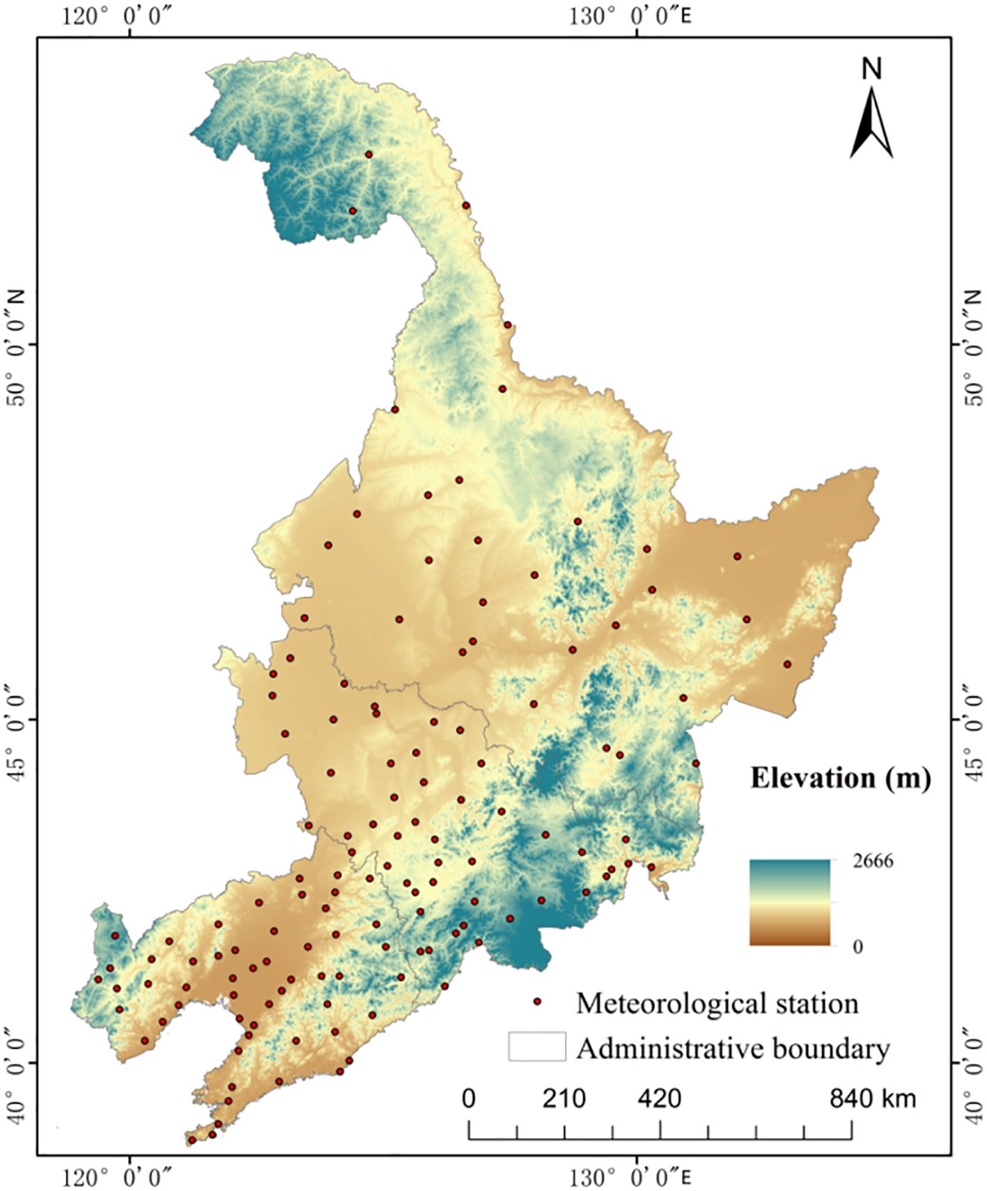
Figure 1. Distribution of the meteorological monitoring points in Northeast China.

2.3 Environmental layers

2.3.1 Climate data

The climate data (temperature, precipitation, snow depth, and solar radiation) used in the study were obtained from the ERA5-Land reanalysis dataset. ERA5-Land is a high-resolution reanalysis dataset released by the European Centre for Medium-Range Weather Forecasts (ECMWF), designed to provide detailed records of meteorological variables over global land surfaces. The ERA5-Land temperature data are generated by assimilating multiple observational sources into a numerical weather prediction model (IFS Cycle 41r2). The model calculates near-surface air temperature (at 2 m height) based on energy balance equations and surface flux parameterizations, incorporating land cover types (vegetation, soil moisture). For ERA5-Land precipitation data, the system combines model forecasts with observational data, optimized through four-dimensional variational assimilation (4D-Var). The ERA5-Land snow depth data are generated through model simulations of snow evolution processes incorporating surface energy balance and snow phase change, while also assimilating satellite-based snow cover observations and in-situ snow depth measurements. The ERA5-Land radiation data are derived from radiative transfer calculations that account for atmospheric composition and cloud interactions (43). The original data are diurnal-scale observations, covering variables such as temperature, precipitation, snow depth, and surface radiation, with a resolution of 0.1°. We undertook a comprehensive preprocessing of the data. First, we calculated the daily mean values for each climate element and simultaneously converted the data into raster format. Second, we separated the daily temperature data into positive and negative values; subsequently, we accumulated these annual data to generate raster datasets representing both the annual positive accumulated temperature (thawing index) and the annual negative accumulated temperature (freezing index). Finally, we calculated and rasterized the annual average values for precipitation, snow depth, and solar radiation. Through this processing approach, five key climate factors were ultimately derived: freezing index, thawing index, snow depth, precipitation, and solar radiation. These variables served as the predictive factors input to the MLMs for subsequent training and establishment.

2.3.2 Soil data

The soil data used in this study were sourced from the Global Soil Dataset for Earth System Modeling (GSDE). This dataset provides comprehensive information about soil attributes, including particle size distribution and organic content. The data is accompanied by quality control indicators, such as confidence levels, to ensure the reliability of the data (44). The spatial resolution of GSDE data is 30 arcseconds. To maintain consistency with the resolution of climate data, the soil element data were resampled to 0.1°. In the vertical direction, this dataset systematically characterized soil properties across eight distinct layers: 0−0.045, 0.045−0.091, 0.091−0.166, 0.166−0.289, 0.289−0.493, 0.493−0.829, 0.829−1.383, and 1.383−2.296 m within a depth of 0 to 2.3 m. Since the bulk density and organic carbon of soil directly control the thermal conductivity, the efficiency of energy transfer in soil is determined. The content of sand and clay regulates the water distribution in soil and affects the release of latent heat from the phase transformation. Gravel content causes a nonlinear effect on freezing by altering water migration paths. Based on the research requirements, we initially screened five soil parameters that held significant environmental relevance as potential predictors: bulk density, organic carbon, sand content, clay content, and gravel content. After undergoing rigorous quality control measures, the soil variables selected provided essential data support for the subsequent model construction.

2.3.3 Digital elevation model

The DEM data used in this study were derived from the geospatial data cloud platform (https://www.gscloud.cn/home). This platform is developed and maintained by the Scientific Data Center of the Computer Network Information Center at the Chinese Academy of Sciences. It serves as a professional online sharing platform that offers a diverse array of geospatial data products. For this study, we selected the ASTER GDEM digital elevation data product, which has a resolution of 30 m. To ensure consistency across datasets, we resampled the original DEM data to align its resolution with that of other climate and environmental element datasets. This processing procedure not only mitigated scale discrepancies among various data sources but also established a unified spatial benchmark for subsequent multi-source data fusion analysis. The DEM contains many factors, in this study we only used the altitude data in the DEM as a position factor, and the elevation values for the study area were all extracted from the DEM.

2.4 Modeling approach

In constructing the model, we thoroughly considered a range of climatic and environmental factors, including the freezing index, thawing index, snow depth, precipitation, solar radiation, digital elevation model (DEM), and soil characteristics (such as bulk density, organic carbon, clay content, gravel content, and sand content). Through feature screening processes, we identified key variables that significantly influenced the freezing depth.

We utilized MFD observations collected from 1975 to 2024 at 123 meteorological monitoring stations located throughout Northeast China. During the model training phase, data from 98 meteorological stations were utilized (with the remaining 25 used for model validation), alongside measured annual MFD data and remote sensing reanalysis data spanning nearly five decades. We systematically trained various MLMs, including RF, support vector machine regression (SVMR), K-nearest neighbor (KNN), and ensemble mean (EM), using dedicated programming tools. The number of training iterations for each method was maintained between 50 and 200 times, while the predictive performance of each model was assessed through spatio-temporal cross-validation and statistical metrics. This approach aimed to identify the optimal machine learning method and training dataset. The techniques were implemented based on the scikit-learn module in Python.

The RF algorithm is an advanced bagging ensemble learning method based on decision trees as weak classifiers. It is a classifier that uses multiple decision trees (a forest) to train and predict samples. This approach is essentially rooted in statistical learning theory, where randomization is applied through resampling: multiple versions of the sample set are extracted from the original training set, a decision tree is trained on each subset, and the results of all trees are combined using a voting mechanism to make the final prediction (45, 46). In this study, the following parameters were used: n_estimators=100, max_depth=5, min_samples_split =10, and max_features = ‘sqrt’.

The SVMR algorithm aims to find an optimal decision hyperplane that not only correctly separates the two categories of data but also maximizes the classification margin between them. Thus, this algorithm exhibits the characteristics of nonlinearity, sparse solutions, and maximum-margin control (47, 48). It assumes an acceptable maximum deviation (ϵ) between the predicted and measured values, for which an ϵ-insensitive loss function is employed to minimize the prediction error. In this study, the following parameters were used: kernel = ‘rbf’, C = 3, gamma = ‘scale’, and epsilon = 0.05. Additionally, normalization methods were applied to avoid overfitting.

The kNN algorithm operates on the principle that, given a known sample space with predefined categories, each new data point is classified based on the k closest samples in the training set. These k samples then determine the category assignment for the new data point (46, 49). In this study, the KNN method identifies the k nearest neighbors for each query point in the samples and uses their average as the prediction value. The parameter k was set to 10, meaning the average of the 10 nearest neighbors was used as the prediction value. Setting the weight parameter to ‘distance’ indicates that each neighbor’s contribution is inversely proportional to its distance.

The EM is to leverage the predictive advantages of different algorithms by assigning different weights to each model to minimize overall bias (50). Specifically, EM first independently trains multiple heterogeneous base learners, then calculates weight coefficients based on each model’s validation set performance, and finally produces outputs that are weighted averages of each model’s predictions. In this study, EM combined three models: RF, SVMR, and KNN.

To address the inherent spatio-temporal autocorrelation of frozen depth data, this study employs a spatio-temporal cross-validation method, which is scientifically justified. Conventional K-fold cross-validation may lead to an overly optimistic evaluation of model performance due to data similarity between adjacent stations and nearby time points. Spatio-temporal cross-validation divides the study area into climate-landform zones and five-decade periods, creating spatial and temporal separation. This method ensures the validation set remains independent of the training set in both spatial and temporal dimensions, thereby providing a more accurate assessment of the model’s predictive ability for unknown spatio-temporal units (51). Since freezing depth is significantly affected by the coupling of local climate and soil conditions, spatio-temporal cross-validation produces more representative data splits for evaluating geographical machine learning models, yielding more reliable model assessments (52, 53).

Based on the training model, we first input annual climate factor data, elevation data, and soil property data into the model. Using our MFD prediction program, we generated predictions on 10 × 10 km grids, with output values obtained through scikit-learn’s prediction method. In the end, we employed an MFD prediction program to generate raster data representing the spatial distribution of MFD on an annual scale in Northeast China. This data was subsequently processed using the ArcGIS platform to derive raster datasets for each adjacent decade (Figures 2–6). Using the resulting raster data, we analyzed the patterns of AMFD variation in Northeast China. The specific research process is shown in Figure 7. To estimate the uncertainty of the predicted values, this study employs a strategy combining bootstrap resampling with multi-round model iteration training. Multiple bootstrap samples were generated from the original dataset. For each bootstrap sample set, we retrained the optimal MLM to construct a probability distribution of freezing depth predictions and determine confidence interval boundaries.

Figure 2

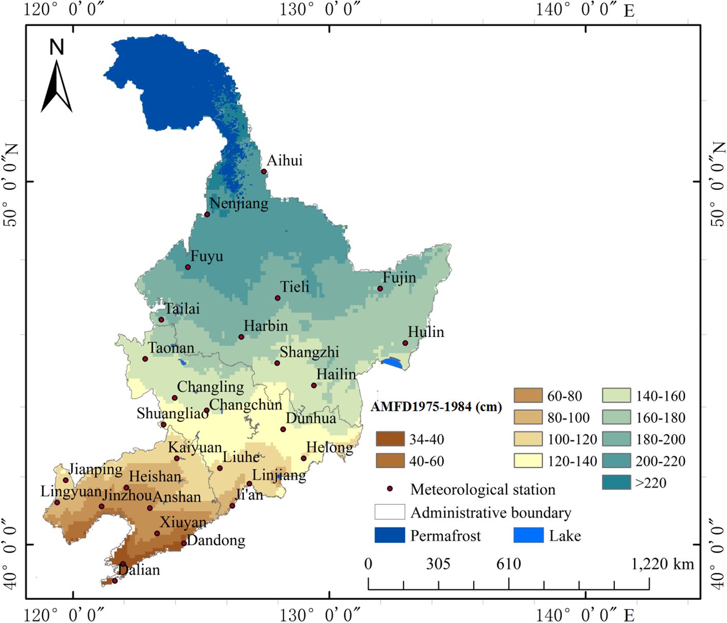
Figure 2. Map of the AMFD from 1975 to 1984.

Figure 3

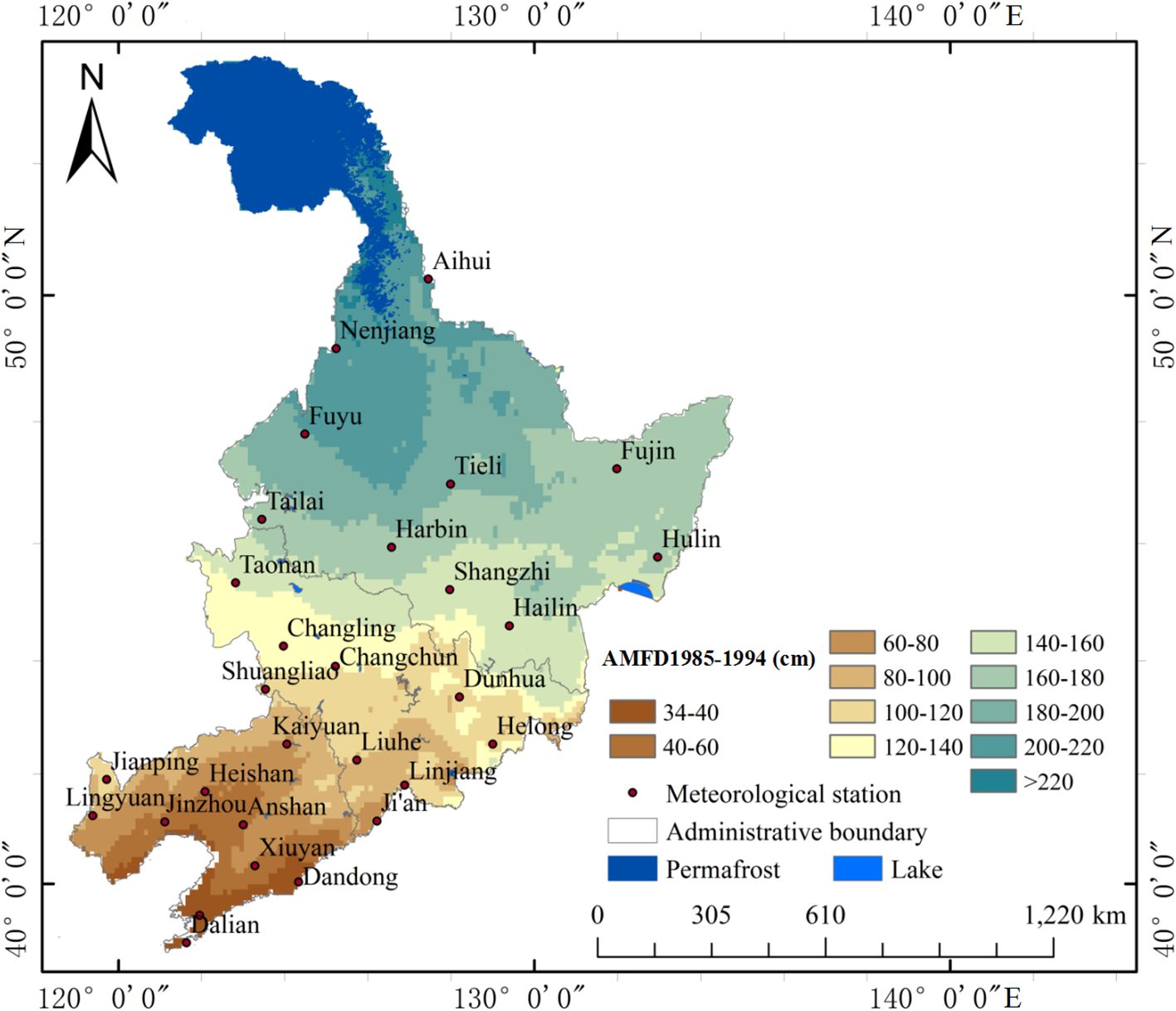
Figure 3. Map of the AMFD distribution from 1985 to 1994.

Figure 4

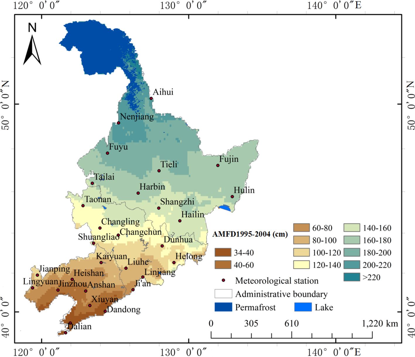
Figure 4. Map of the AMFD distribution from 1995 to 2004.

Figure 5

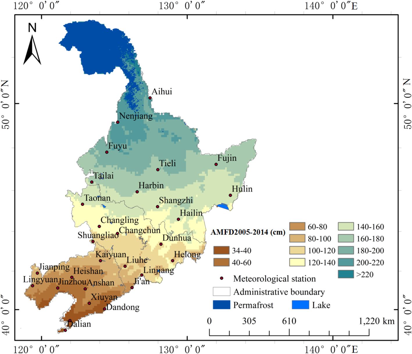
Figure 5. Map of the AMFD distribution from 2005 to 2014.

Figure 6

Figure 6. Map of the AMFD distribution from 2015 to 2024.

Figure 7

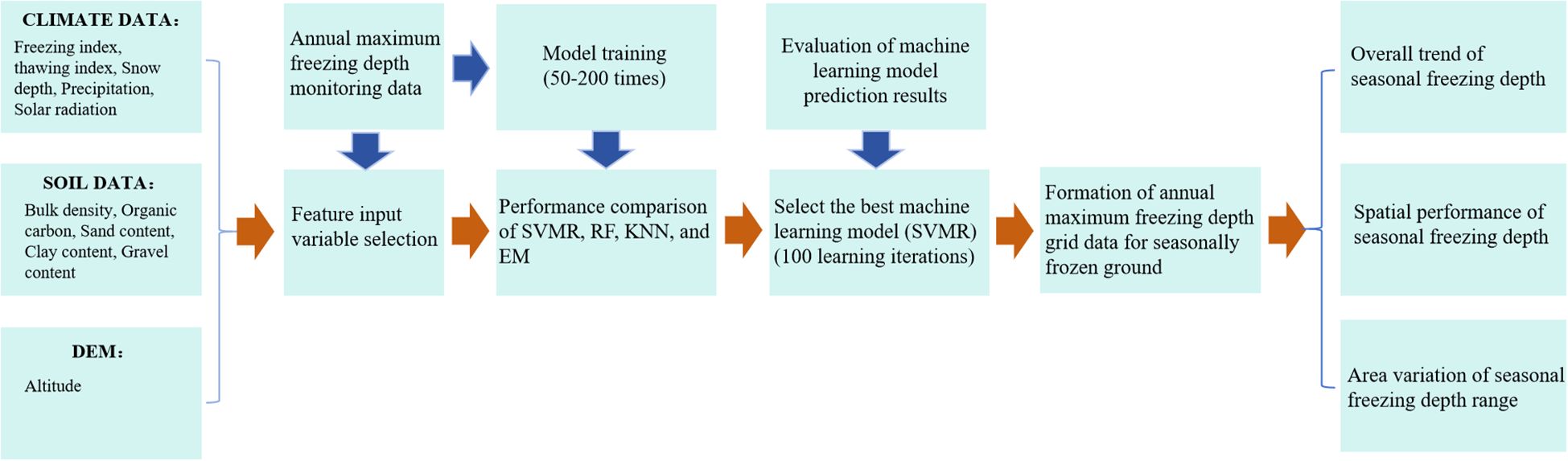
Figure 7. The research process used to assess freezing depth variation.

2.5 Uncertainty estimation

To evaluate uncertainty estimation, we adopted a method combining bootstrap resampling and model retraining. First, bootstrap samples were generated by randomly resampling the original dataset. For each bootstrap sample, we retrained the optimal SVMR model (with 100 training repetitions) to obtain the distribution of freezing depth prediction values. We then used the 5th and 95th percentiles of predicted values to establish a 90% confidence interval. Second, we utilized existing 50–200 training repetition sets for each algorithm along with periodic standard deviation measurements to evaluate the model’s internal stability.

The 50-year (1975-2024) average maximum freezing depth map of Northeast China is shown in Figure 8, and the uncertainty map is shown in Figure 9. We computed a 90% Confidence Interval (CI) widths from 100 bootstrap iterations and Identified high-uncertainty zones. We Used sequential colormap (Yellow-Red) to represent CI magnitude, with a gray line to isolate of high uncertainty.

Figure 8

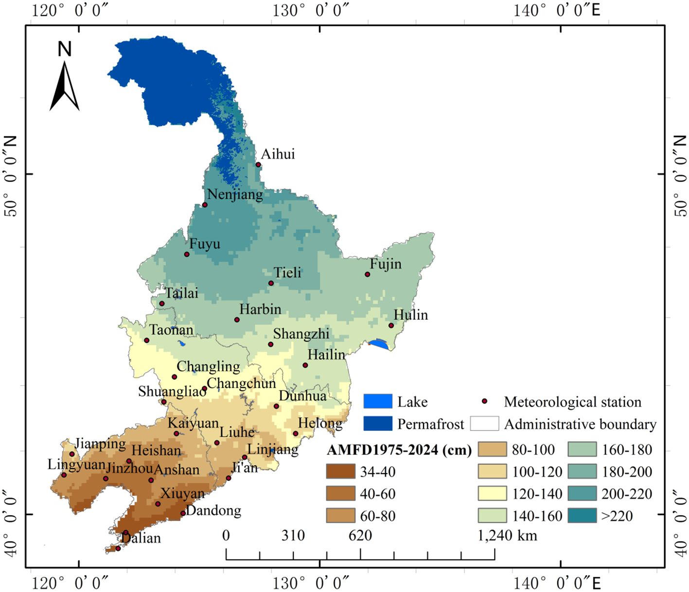
Figure 8. Map of the AMFD from 1975 to 2024.

Figure 9

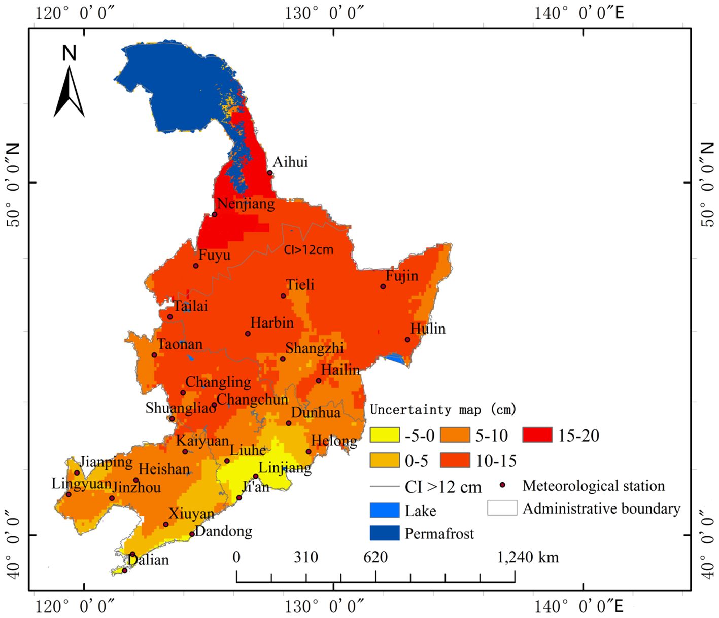
Figure 9. Uncertainty map of the AMFD from 1975 to 2024.

A threshold that is too low may include too many low-risk areas, while a threshold that is too high may overlook genuine risks. In this study, the CI width was set at 12 cm, indicating that the true value may vary by ±6 cm. Areas with a CI > 12 cm are classified as high-uncertainty zones, where the 90% confidence interval exceeds 12 cm. This threshold was determined based on the 75th percentile of bootstrapping results and the average error of freezing depth monitoring equipment in Northeast China.

Additionally, according to China’s current Code for Engineering Geological investigation of Frozen Ground (GB50324-2014) (54), a frost heave rate of 3% is classified as weak frost heave, posing minimal impact on engineering structures in permafrost regions. For areas with freezing depths below 50 cm, replacement methods are applicable. In high-freezing-depth areas (e.g., 2 m), a 3% frost heave rate translates to 6 cm of deformation. Thus, the defined confidence interval represents an engineering-critical error margin deemed acceptable in practice.

3 Results

3.1 Feature selection

In the process of establishing MLMs, the selection of feature input variables is a key link that determines the performance of the model. Reasonable variable selection can not only improve the prediction accuracy and generalization ability of the model, but also effectively accelerate the convergence speed of the model. This is very important for studying the changes in the freezing depth of SFG using MLMs. The Permutation Importance Evaluation Method quantifies feature importance by randomly shuffling individual feature values and observing the resulting degradation in model performance. The implementation process comprised four key steps: (1) During data preprocessing, all continuous variables were standardized using “z-score normalization”, while categorical variables were one-hot encoded; (2) An Extra-Trees regressor was trained on 70% of the training dataset; (3) After calculating the baseline mean squared error (MSE₀) on an independent test set, each feature column was sequentially shuffled, and the error (MSE_i) was recalculated, with the feature importance score defined as I_i = MSE_i - MSE₀; (4) To reduce stochastic variability, the experiment was repeated 10 times, and the mean was taken, while statistically insignificant variables were excluded using a one-sample t-test (α = 0.05). Using this approach (22), we conducted an importance ranking analysis on the initially set of 11 potential predictors [freezing index, thawing index, precipitation, snow depth, solar radiation, DEM (altitude), bulk density, organic carbon, sand content, clay content and gravel content]. The results indicated (Figure 10) that among the various factors influencing the freezing depth of SFG in Northeast China, the freezing index made the most significant contribution, followed by solar radiation. The thawing index and DEM (altitude) had the same degree of influence. This ranking result has significant physical implications. As fundamental indicators that characterize climatic conditions, the freezing index and thawing index played a crucial role in the development of SFG. This finding was closely aligned with the conclusions of several previous studies, indicating that climate change has had a substantial impact on the variation in depth (55, 56). Comprehensively considering the ranking results of the importance of characteristic factors and their practical physical significance, we ultimately identified eight representative predictors to serve as input variables for the MLM. These predictors were freezing index, solar radiation, thawing index, DEM (altitude), snow depth, precipitation, bulk density, and gravel content. These characteristic factors encompassed the essential environmental elements, including climatic conditions (freezing/thawing index, solar radiation, snow depth, and precipitation), topographic features (DEM), and soil properties (bulk density and gravel content). Collectively, these factors provided a comprehensive reflection of the multi-dimensional environmental characteristics that influence the development of SFG.

Figure 10

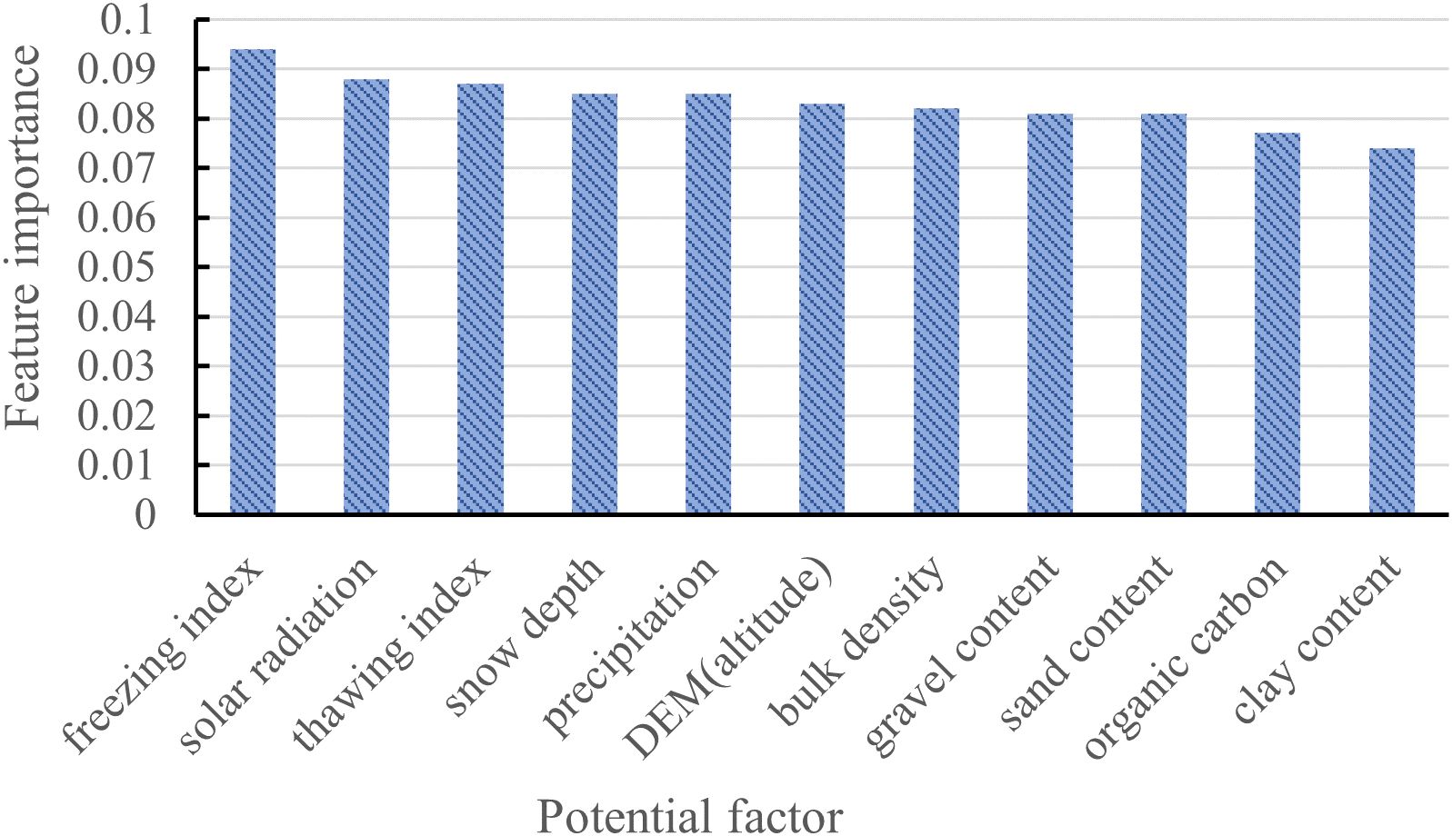
Figure 10. Ranking the importance of the input variables.

3.2 Model interpretation

Using climate and remote sensing data as input variables, we adopted multiple machine learning methods to predict and model the freezing depth of SFG. Specifically, four algorithms were selected for a comparative analysis: RF, SVMR, KNN, and EM. Table 1 presents the performance metrics of each model, evaluated through the coefficient of determination (R²), root mean square error (RMSE), mean absolute error (MAE), and bias. The results of the comparative analysis showed that in terms of prediction accuracy, the overall performance of the three methods, i.e., RF, SVMR, and EM, was significantly better than that of the KNN method. In terms of the R², the SVMR and EM methods demonstrated significant advantages. When the number of training iterations reached 100, their R² values were markedly higher than those obtained from the RF and KNN methods. To ensure a robust model evaluation, we further analyzed the characteristics of the error indices. Given that the RMSE is more sensitive to outliers, whereas the MAE provides a more stable reflection of prediction error, we prioritized the SVMR method with the smallest MAE value when the training iterations were set to 100 and the RMSE values across models were similar. Notably, SVMR demonstrated a more stable error control ability while maintaining a relatively high R² value. A training session consisting of 100 iterations not only ensured that the model comprehensively learnt the data features but also mitigated the risk of overfitting. Compared with other methods, SVMR had the advantages of being able to deal with nonlinear relationships and small sample sizes. It was suitable for problems with complex environmental influencing factors, such as freezing depth prediction. After comprehensively considering the accuracy and stability of the models, we finally adopted the SVMR model trained 100 times as the optimal prediction model. The design of the training process being repeated 50–200 times in this study is based on the following considerations: First, to eliminate the impact of randomness on model performance evaluation through multiple runs. Second, when the number of training iterations exceeds 100, the standard deviations of R² and MAE for each model tend to stabilize, indicating that further increases in the number of iterations have a limited effect on improving reliability.To enhance model interpretability and gain deeper insights into feature contribution mechanisms, we employed Shapley Additive Explanations (SHAP) to assess the marginal impact of each feature on model predictions (Table 2). The assessment indicates that the freezing index, solar radiation, and thawing index are key factors influencing freezing depth prediction, while large absolute SHAP values align with the energy balance theory of frozen ground. The accumulative negative temperature directly promotes frozen ground development, with its highest SHAP value reflecting its core driving role. Conversely, accumulative positive temperature and increased radiation lead to surface warming, thereby reducing freezing depth, showing significant negative contributions. The contributions of snow depth, precipitation, and DEM to freezing depth prediction cannot be ignored either: snow depth exhibits both a strong insulating effect and high surface reflectivity, which weakens the freezing effect; winter precipitation increases soil moisture, promoting soil freezing; while high-altitude areas experience lower temperatures, further promoting soil freezing. The mean SHAP values of soil parameters (bulk density and gravel content) are relatively low, suggesting that their influence on freezing depth is mediated through heat conduction and moisture migration, making these complex coupling processes difficult for the model to capture.

Table 1

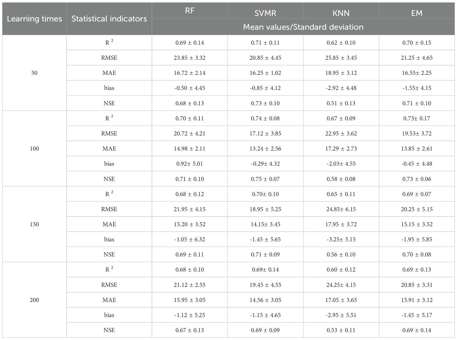
Table 1. Mean values and standard deviation of the statistical indicators of various MLMs.

Table 2

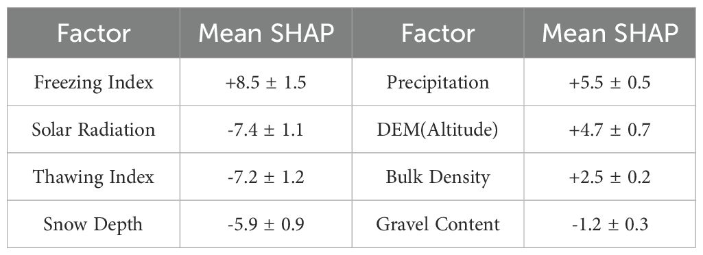
Table 2. Key factor and SHAP values.

3.3 Evaluation of the predictive ability of SVMR

This study employed a spatio-temporal cross-validation method, beginning with spatial partitioning. Due to the relatively independent climate-geomorphology characteristics of the three provinces in northeast China, the 98 training points were divided into 3 spatial subsets according to provincial boundaries. This ensures that the spacing between sites within each subset meets the required criteria to maintain spatial coherence. Next, within each spatial subset, the 50 years of data were grouped into five 10-year periods for temporal stratification. For each iteration, one space-time combination was used as the test set in sequence, while the other combinations served as training sets for iterative training. Finally, the average and standard deviation of NSE values obtained from each validation were calculated.

The optimized NSE values (Table 1) show that the SVMR model achieves an NSE of 0.75 ± 0.07 (based on 100 training sessions), indicating that the kernel function effectively captures the key spatio-temporal interaction characteristics of frozen ground formation through nonlinear mapping, while the regularization parameter helps suppress overfitting across the data period. Among the other models, the EM algorithm performs suboptimally due to the inherent limitations of ensemble learning (NSE=0.73 ± 0.06), whereas KNN is constrained by the local smoothing assumption (NSE=0.58 ± 0.08), resulting in strong spatial heterogeneity. These results demonstrate that NSE values obtained through spatio-temporal cross-validation can reliably assess the model’s generalization ability in unknown spatio-temporal scenarios.

Based on the raster data for the 10-year AMFD, we extracted the predicted values for 25 meteorological monitoring points in Northeast China. These values were then compared against the mean observation data from the same period (Figure 11). The R² between the predicted and observed values from 1975 to 1984, 1985 to 1994, 1995 to 2004, 2005 to 2014, and 2015 to 2024 all exceeded 86%, and all passed a significance test at P <0.01. These results suggested that the combination of an MLM with remote sensing reanalysis data resulted in a good fitting performance in predicting the MFD of SFG. The predicted values yielded by the model showed good spatial consistency with the observed values from meteorological stations, enabling an accurate representation of the actual seasonal freezing depth conditions in Northeast China.

Figure 11

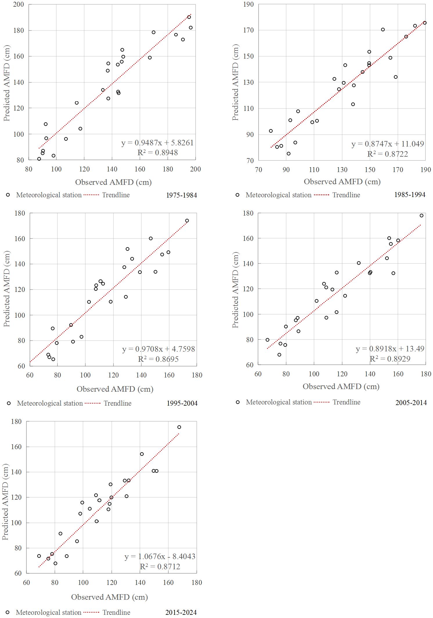
Figure 11. Comparison of predicted and observed values from 1975 to 2024.

3.4 Overall trend of AMFD

The overall variation in the AMFD of SFG in Northeast China from 1975 to 2024 is shown in Figure 12. There was a significant decreasing trend in AMFD in the region, with the rate of change measured at -8.54 cm/10a. The AMFDs in Northeast China were 136.71 cm (1975−1984), 131.96 cm (1985−1994), 123.07 cm (1995−2004), 110.82 cm (2005−2014), and 104.58 cm (2015−2024). The reductions in the AMFD between each adjacent decade were 4.75 cm (1975−1984 to 1985−1994), 8.89 cm (1985−1994 to 1995−2004), 12.25 cm (1995−2004 to 2005−2014), and 6.24 cm (2005−2014 to 2015−2024). The AMFD changed most substantially during the 20 years from 1995 to 2014. The decrease in the AMFD between 1995−2004 and 2005−2014 reached 12.25 cm. The reduction in the AMFD between 1985−1994 and 1995−2004 was 8.89 cm, while the rate of AMFD reduction between 2005−2014 and 2015−2024 slowed-down, with the reduction in the AMFD being 6.24 cm.

Figure 12

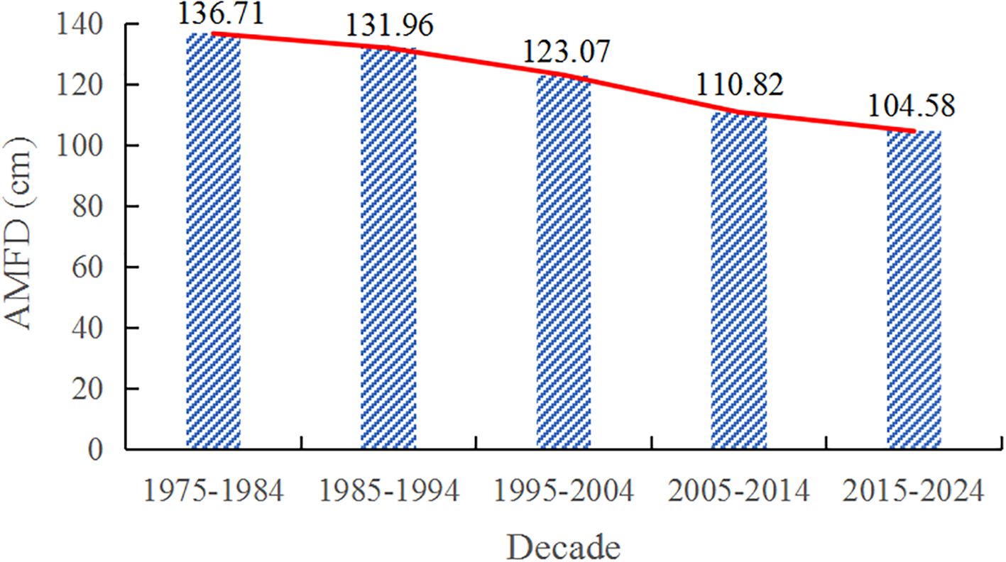
Figure 12. The AMFD in Northeast China over 5 decades.

3.5 Spatial distribution of the AMFD

Figure 2 is a map of the AMFD distribution in Northeast China from 1975 to 1984. The AMFD remained within 40−220 cm and increased with an increase in latitude. The AMFD interval of 40−60 cm was distributed to the south of Jinzhou, Xiuyan, and Dandong. The AMFD of the SFG located south of Heishan and Anshan remained within 60−80 cm. The AMFD in the area north of Anshan and Ji ‘an to the south of Kaiyuan and Linjiang reached 80−100 cm, while in the area north of Linjiang and Liuhe, the AMFD reached 100−120 cm. The AMFD in the area north of Shuangliao and south of Changchun and Dunhua remained within 120−140 cm. A dividing line, stretching from Taonan to Shangzhi to Hailin separated the regions with AMFD intervals of 140−160 and 160−180 cm. The AMFD north of the line of Tailai, Harbin, and Fujin reached 180−200 cm. The AMFD south of Fuyu, Nenjiang, and Aihui exceeded 200 cm, and the AMFD in some areas around Nenjiang and Aihui exceeded 220 cm.

The AMFD map from 1985 to 1994 (Figure 3) was compared with the AMFD map from 1975 to 1984 (Figure 2). During this period, the AMFD in the eastern part of Jinzhou, the southern part of Heishan, and the western part of Anshan decreased from 60−80 to 40−60 cm. The AMFD in the Kaiyuan-Liuhe-Linjiang area decreased from 100−120 to 80−100 cm. The AMFD interval of 120−140 cm was largely replaced by the AMFD interval of 100−120 cm. The area with an AMFD interval of 140−160 cm in the northern part of Shangzhi and the western part of Hailin expanded over the period investigated, while the area with an AMFD of 160−180 cm decreased. In the northeastern, western, and northwestern regions of Fujin, the AMFD interval of 180−200 cm was replaced by the AMFD interval of 160−180 cm. Additionally, the extent of the AMFD interval of 200−220 cm in the northern area of Tieli contracted over the period investigated to encompass only the southern region of Aihui, indicating a relatively significant reduction in this interval.

The AMFD map from 1995 to 2004 (Figure 4) was compared with the AMFD map from 1985 to 1994 (Figure 3). During this period, the AMFD in some areas between the northwest of Ji ‘an and the southeast of Liuhe decreased from 100−120 to 80−100 cm. In the area between the eastern part of Changchun and the northwestern part of Dunhua, a local expansion phenomenon occurred in the area with an AMFD interval of 120−140 cm, and the area with an AMFD interval of 100−120 cm decreased. The area with an AMFD interval of 140−160 cm in the southern region of Shangzhi decreased slightly over the period investigated. Similarly, the area with an AMFD interval of 160−180 cm in the northern part of Hailin also decreased slightly. The area with an AMFD interval of 180−200 cm around Tieli decreased significantly. In the southeastern to northeastern regions of Fuyu, the area with an AMFD interval of 200−220 cm displayed a substantial reduction.

The AMFD map for 2005−2014 (Figure 5) shows a slight expansion in the area with an AMFD interval of 100−120 cm in the southern part of Changchun when compared to the AMFD map from 1995−2004. The area with an AMFD interval of 140−160 cm in the northeastern part of Changling decreased during this period. The area with an AMFD interval of 140−160 cm between Dunhua and Hailin experienced a significant reduction. In most regions of northwest Hulin and southern Fujin, the AMFD contracted from 160−180 to 140−160 cm.

The AMFD map from 2015 to 2024 (Figure 6) shows a local expansion phenomenon in the area with an AMFD interval of 40−60 cm in the northern part of Anshan compared with the AMFD map from 2005 to 2014. The area with an AMFD interval of 60−80 cm in the southern region of Kaiyuan exhibited localized expansion. A slight expansion phenomenon occurred in the area with an AMFD interval of 100−120 cm in the southern region of Liuhe. The area with an AMFD interval of 140−160 cm in the western region of Fujin expanded, while the area with an AMFD interval of 160−180 cm decreased. In contrast, the AMFD around Tailai and Harbin remained stable within the interval of 160−180 cm.

3.6 Variations in the areas of AMFD intervals

The distribution of the areas corresponding to various AMFD intervals in Northeast China is shown in Figure 13. Over the past 50 years, the area with an AMFD of <160 cm displayed an increasing trend. The expansion of these areas was notable, with increases of 1,700 km² (<40 cm), 8,500 km² (40−60 cm), 25,600 km² (60−80 cm), 26,200 km² (80−100 cm), 38,800 km² (100−120 cm), 44,700 km² (120−140 cm), and 63,200 km² (140−160 cm). The area with an AMFD of >160 cm displayed a decreasing trend. The reduction of these areas was also notable, with decreases of 64,500 km² (160−180 cm), 88,100 km² (180−200 cm), and 56,200 km² (>200 cm). The area with an AMFD interval of 140−160 cm increased the most, followed by an AMFD interval of 120−140 cm. In contrast, the increase in the area with an AMFD of <40 cm was minimal. Conversely, the area with an AMFD interval of 180−200 cm decreased significantly, with a notable reduction also observed in the area with an AMFD interval of 160−180 cm. The decrease in areas with an AMFD of >200 cm was comparatively smaller.

Figure 13

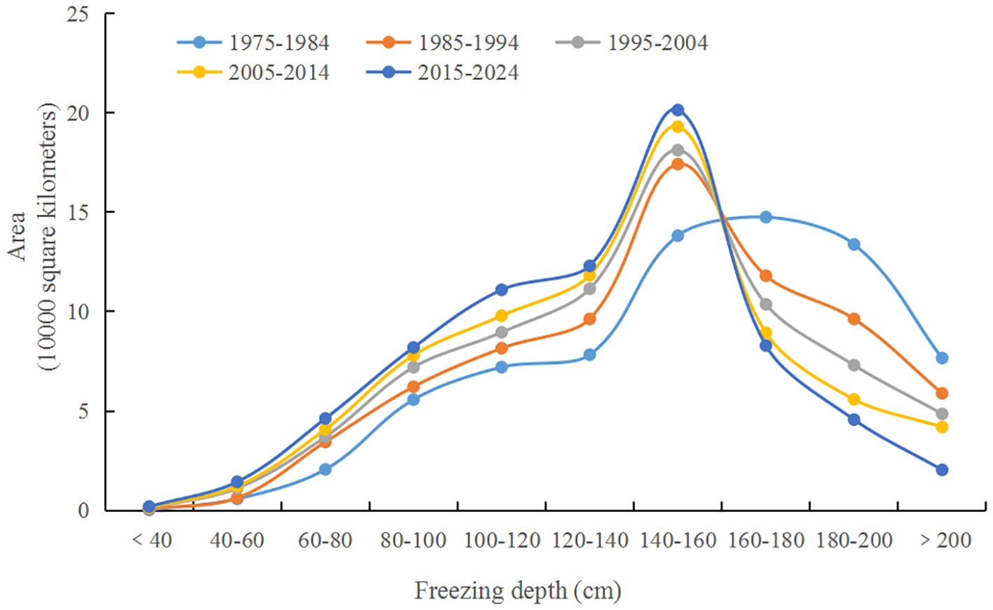
Figure 13. Variations in the area of different AMFD intervals.

4 Discussion

A comprehensive evaluation of the performance of MLMs was conducted based on a spatio-temporal cross-validation method. Various statistical assessment metrics indicated that the newly developed machine learning prediction model demonstrated high accuracy and reliability. Unlike conventional empirical models (57–59), MLMs can effective capture of the complex nonlinear relationships between various environmental factors, such as climate variables and soil characteristics, and freezing depth. Therefore, compared with empirical models that require calibration for different geographical and climatic conditions, MLMs demonstrate distinct advantages. Remote sensing reanalysis data provided continuous and consistent environmental scenarios. The acquisition of such continuous data not only compensated for the spatial coverage limitations of traditional observational data but also helped to smooth out the effects of long-term fluctuations. Furthermore, it highlighted the trends in seasonal freezing depth changes over extended periods. The NSE results show that the kernel function of SVMR effectively captures the key spatio-temporal interaction characteristics of frozen ground formation through nonlinear mapping, while the regularization parameter effectively suppresses overfitting across the data period. These results indicate that NSE values obtained through spatio-temporal cross-validation can reliably assess the model’s generalization ability for unknown spatio-temporal scenarios. The model maintained a stable predictive performance over the past 50 years (1975−2024), indicating that a strong capacity for temporal extrapolation was inherent in machine learning. This study systematically evaluated the prediction uncertainty by combining bootstrap resampling and multi-round model training. We computed 90% CI widths from 100 bootstrap iterations and identified high-uncertainty zones. Notably, the model’s internal stability analysis revealed that SVMR exhibited a consistently lower standard deviation in repeated training compared to other algorithms, indicating better reproducibility in its predictions. These findings provide important insights for error control in subsequent research.

Permutation importance analysis revealed that the freezing index, solar radiation, and thawing index are the dominant factors influencing freezing depth variations. As fundamental climate indicators, the freezing index and thawing index directly respond to climate change, which can significantly impact freezing depth (55, 56). Additionally, snow depth and precipitation play significant roles in freezing depth dynamics. Snow depth insulates energy exchange between the ground and atmosphere, while its thermal effects alter frozen ground properties, thereby affecting freezing depth variations (60). Precipitation modifies the moisture content of frozen ground. These findings enhance our understanding of the frozen soil-climate feedback mechanism.

The analysis of the AMFD of SFG in Northeast China from 1975 to 2024 revealed that the changes over nearly 5 decades exhibited distinct phase characteristics. This indicated that the process of decreasing freezing depth in this region was not uniform but rather occurred in a non-linear manner. The period from the mid-1990s to the early 21^st century was the time when the freezing depth of SFG in this region changed most intensely. Although the degradation rate has slowed down in the last decade, the general trend for a continuous shallower freezing depth of SFG has not changed. The research findings have important implications for regional sustainable development. For urban development, the continuous decrease in freezing depth may reduce the stability standards for foundations, requiring greater attention to frost heave risk (6–8). In the agricultural sector, a shortened soil freeze period could extend the growing season for crops while also increasing the risk of spring floods, which would require adjustments in farming systems and improvements in drainage facilities (10, 17).

Additionally, this study has several limitations. The spatial resolution of soil data (10 km) limits the ability to capture small-scale heterogeneity, especially in the farmland-forest ecotone of northeast China. The model does not account for human-induced thermal disturbances in localized areas, such as the urban heat island effect, which may lead to underestimation of freezing depth reduction rates in densely urbanized areas. Furthermore, the interaction mechanism between permafrost and SFG was not incorporated into the model framework. Future studies could enhance model performance by integrating multi-source satellite data and improving the parameterization scheme for soil thermal conductivity. These improvements would be particularly important for accurately predicting frozen ground degradation processes near the “critical climate threshold”. Despite these limitations, this study provides the optimal machine learning framework for predicting seasonal freezing depth in northeast China given the current data availability.

5 Conclusion

This study reveals the spatio-temporal variations of the MFD of SFG in Northeast China from 1975 to 2024 using MLMs. In the past 50 years, the AMFD in Northeast China displayed a decreasing trend, with an average decrease of -8.54 cm/10a. The spatial distribution of different freezing depth intervals has undergone significant adjustments. Among these regions, the area with freezing depth shallower than 160 cm continues to expand, while the area with freezing depth exceeding 160 cm has significantly decreased, particularly in northern Tailai, eastern Fuyu, and along the Nenjiang, where degradation is most severe. This change is closely associated with rising winter temperatures, a shortened snow cover period, and increased soil moisture in Northeast China under global warming (18). The freezing depth phase characteristics further demonstrate the sensitivity of the frozen ground system to climate change. The SVMR model developed in this study performs well in predicting freezing depth.

The spatio-temporal variation of MFD in Northeast China has significant scientific value. On the one hand, the continuous reduction of freezing depth directly affects the stability of foundations in cold regions, necessitating precautions against long-term settlement risks caused by the weakening of frost heave forces. On the other hand, degradation of frozen ground may alter regional hydrological cycles, thereby impacting agricultural irrigation and flood prevention strategies.

While this study has certain limitations, future research could incorporate high-resolution urban heat island effect data to better quantify anthropogenic impacts on freezing depth reduction. Additionally, implementing physically constrained deep learning frameworks could further enhance model extrapolation capabilities for extreme climate scenarios.

Data availability statement

The original contributions presented in the study are included in the article/supplementary material. Further inquiries can be directed to the corresponding author.

Author contributions

SW: Writing – original draft, Methodology, Writing – review & editing. AT: Investigation, Writing – review & editing. NM: Investigation, Writing – review & editing. Z-JN: Supervision, Writing – review & editing.

Funding

The author(s) declare financial support was received for the research and/or publication of this article. This research was funded by the China National Natural Science Foundation (No. 52068035)

Conflict of interest

The authors declare that the research was conducted in the absence of any commercial or financial relationships that could be construed as a potential conflict of interest.

Generative AI statement

The author(s) declare that no Generative AI was used in the creation of this manuscript.

Publisher’s note

All claims expressed in this article are solely those of the authors and do not necessarily represent those of their affiliated organizations, or those of the publisher, the editors and the reviewers. Any product that may be evaluated in this article, or claim that may be made by its manufacturer, is not guaranteed or endorsed by the publisher.

References

1. Zhao L, Cheng GD, and Ding YJ. Studies on frozen ground of China. J Geogr Sci. (2004) 14:411–6. doi: 10.1007/BF02837484

Crossref Full Text | Google Scholar

2. Xu S, Liu D, and Li TX. Spatiotemporal evolution of the maximum freezing depth of seasonally frozen ground and permafrost continuity in historical and future periods in Heilongjiang Province, China. Atmospheric Res. (2022) 274:106195. doi: 10.1016/j.atmosres.2022.106195

Crossref Full Text | Google Scholar

3. Huang S, Ding Q, and Chen KZ. Changes in near-surface permafrost temperature and active layer thickness in Northeast China in 1961–2020 based on GIPL model. Cold Regions Sci Technology. (2023) 206:103709. doi: 10.1016/j.coldregions.2022.103709

Crossref Full Text | Google Scholar

4. Mi X, Zhang W, Zhang G, and Wang X. Study on anti-frost heave effect of new thermal insulation subgrade of highway in seasonally frozen soil regions. PloS One. (2025) 20:e0318682. doi: 10.1371/journal.pone.0318682

PubMed Abstract | Crossref Full Text | Google Scholar

5. Qiu GQ and Liu JG. Dictionary of frozen soil science (Chinese, english, Russian). Lanzhou, China: Gansu Science and Technology Press (1994).

Google Scholar

6. Lu B, Zhao W, Li S, Dong M, Xia Z, and Shi Y. Study on seasonal permafrost roadbed deformation based on water–heat coupling characteristics. Buildings. (2024) 14:2710. doi: 10.3390/buildings14092710

Crossref Full Text | Google Scholar

7. Zhang BQ, Tian MJ, and Li X. The Impact of natural diseases on highway construction in Xinjiang. Chin Foreign Highways. (2005) 25:3. doi: 10.3969/j.issn.1671-2579.2005.02.004

Crossref Full Text | Google Scholar

8. Niu F, Hu H, Liu M, Ma Q, and Su W. Studies for frost heave characteristics and the prevention of the high-speed railway roadbed in the Zoige Wetland, China. Front Earth Sci. (2021) 9:655–78. doi: 10.3389/feart.2021.678655

Crossref Full Text | Google Scholar

9. Song LQ, Zang SY, and Lin L. Responses of nitrous oxide fluxes to autumn freezing-thaw cycles in permafrost peatlands of the Da Xing’ an mountains, Northeast China. Environ Sci pollut Control Ser. (2022) 29:31700–12. doi: 10.1007/s11356-022-18545-z

PubMed Abstract | Crossref Full Text | Google Scholar

10. He YH. Study on the Effects of Different Freeze Thaw Cycle Conditions on Soil Structure and Moisture Characteristics in Farmland. Master’s Thesis, Northeast Agricultural University, China. (2023) doi: 10.27010/d.cnki.gdbnu.2023.000607

Crossref Full Text | Google Scholar

11. Qin Y, Chen J, Yang D, and Wang T. Estimating seasonally frozen ground depth from historical climate data and site measurements using a Bayesian model. Water Resour Res. (2018) 54:4361–75. doi: 10.1029/2017WR022185

Crossref Full Text | Google Scholar

12. Zhang T, Barry RG, and Knowles K. Statistics and characteristics of permafrost and ground-ice distribution in the Northern Hemisphere: Polar Geography. Polar Geogr. (2008) 31:1–12. doi: 10.1080/10889370802175895

Crossref Full Text | Google Scholar

13. Wang X, Chen RS, and Yang Y. Effects of permafrost degradation on the hydrological regime in the source regions of the yangtze and yellow rivers, China. Water. (2017) 9:897. doi: 10.3390/w9110897

Crossref Full Text | Google Scholar

14. Zhang T, Barry RG, and Knowles K. (2003). Distribution of seasonally and perennially frozen ground in the Northern Hemisphere, in: Proceedings of the 8th International Conference on Permafrost, Lisse, Netherlands: Balkema Publishers Vol. 2. pp. 1289–94.

Google Scholar

15. Streletskiy DA, Shiklomanov NI, and Nelson FE. Spatial variability of permafrost active-layer thickness under contemporary and projected climate in Northern Alaska. Polar Geogr. (2012) 35:95–116. doi: 10.1080/1088937X.2012.680204

Crossref Full Text | Google Scholar

16. Yue SP, Yan YH, Zhang SW, Yang JH, and Wang WJ. Spatiotemporal variations of soil freeze-thaw state in Northeast China based on the ERA5-LAND dataset. Acta Geographica Sin. (2021) 76:2765–79. doi: 10.11821/dlxb202111012

Crossref Full Text | Google Scholar

17. Li R, Zhao L, Ding Y, Wu T, Xiao Y, Du E, et al. Temporal and spatial variations of the active layer along the Qinghai-Tibet Highway in a permafrost region. Chin Sci Bull. (2012) 57:8. doi: 10.1007/s11434-012-5323-8

Crossref Full Text | Google Scholar

18. Liaoning Meteorological Bureau. Second assessment report on climate change in Northeast China. Shenyang: Liaoning Provincial Government (2021).

Google Scholar

19. Lunardini VJ. Heat transfer in cold climates. New York: Van Nostrand Reinhold (1981).

Google Scholar

20. Kudrayavtsev VA. Osnovy merzlotnogo prognoza. Moscow: Moscow University Press (1974).

Google Scholar

21. Lundberg SM and Lee SI. (2017). A unified approach to interpreting model predictions, in: Advances in Neural Information Processing Systems. Red Hook, NY, United States: Curran Associates Inc.

Google Scholar

22. Wang B and Ran Y. Diversity of remote sensing-based variable inputs improves the estimation of seasonal maximum freezing depth. Remote Sens. (2021) 13:4829. doi: 10.3390/rs13234829

Crossref Full Text | Google Scholar

23. Ran Y, Li X, Cheng G, Che J, Aalto J, Karjalainen O, et al. New high-resolution estimates of the permafrost thermal state and hydrothermal conditions over the Northern Hemisphere. Earth Syst Sci Data Discuss. (2021) 21:1–27. doi: 10.5194/essd-2021-83

Crossref Full Text | Google Scholar

24. Ran Y and Li X. Progress, chanllenges and opportunities of permafrost mapping in China. Adv Earth Sci. (2019) 34:1015–27. doi: 10.11867/j.issn.1001-8166.2019.10.1015

Crossref Full Text | Google Scholar

25. Jan A and Painter SL. Permafrost thermal conditions are sensitive to shifts in snow timing. Environ Res Lett. (2020) 15:084026. doi: 10.1088/1748-9326/ab8ec4

Crossref Full Text | Google Scholar

26. Liu Z, Chen B, Wang S, Wang Q, Chen J, Shi W, et al. The impacts of vegetation on the soil surface freezing-thawing processes at permafrost southern edge simulated by an improved process-based ecosystem model. Ecol Model. (2021) 456:109663. doi: 10.1016/j.ecolmodel.2021.109663

Crossref Full Text | Google Scholar

27. Zhang YL, Cheng GD, and Li X. Coupling of a simultaneous heat and water model with a distributed hydro logical model and evaluation of the combined model in a cold region watershed. Hydrol. Process. (2013) 27:3762–76. doi: 10.1002/hyp.9514

Crossref Full Text | Google Scholar

28. Azeem MA and Dev S. A performance and interpretability assessment of machine learning models for rainfall prediction in the Republic of Ireland. Decision Analytics J. (2024) 12:100515. doi: 10.1016/j.dajour.2024.100515

Crossref Full Text | Google Scholar

29. Rafael GS, Cassio M, Marcio R, and Carlos EGR. Machine learning applied for Antarctic soil mapping: Spatial prediction of soil texture for Maritime Antarctica and Northern Antarctic Peninsula. Geoderma. (2023) 432:116405. doi: 10.1016/j.geoderma.2023.116405

Crossref Full Text | Google Scholar

30. Li KQ and He HL. Towards an improved prediction of soil-freezing characteristic curve based on extreme gradient boosting model. Geosci Front. (2024) 15:101898. doi: 10.1016/j.gsf.2024.101898

Crossref Full Text | Google Scholar

31. Park S and Choe Y. Cho, H.i; Pham, K. Machine learning-based pseudo-continuous pedotransfer function for predicting soil freezing characteristic curve. Geoderma. (2025) 453:117145. doi: 10.1016/j.geoderma.2024.117145

Crossref Full Text | Google Scholar

32. Han XL, Liu JT, Wu PF, and Yu ZH. Predicting the thickness of alpine meadow soil on headwater hillslopes of the Qinghai-Tibet Plateau. Geoderma. (2025) 456:117271. doi: 10.1016/j.geoderma.2025.117271

Crossref Full Text | Google Scholar

33. Wang B and Ran Y. Prediction of future changes in maximum freezing depth of permafrost during the third polar season based on machine learning. J Glaciology Geocryology. (2023) 7:1–10. doi: 10.7522/j.issn.1000-0240.2023.0061

Crossref Full Text | Google Scholar

34. Sun FH, Li LG, and Zhang YC. Key zone, key period and key factor influencing climate in Northeast China. Scientia Geographica Sin. (2011) 31:911–6. doi: 10.13249/j.cnki.sgs.2011.08.911

Crossref Full Text | Google Scholar

35. Gong Q, Chao H, and Zhu L. Refined analysis of spatiotemporal characteristics of ground temperature and freezing depth in Northeast China. J Glaciology Geocryology. (2021) 43:1782–93. doi: 10.7522/j.issn.1000-0240.2021.0052

Crossref Full Text | Google Scholar

36. Wang CH, Jin SL, and Shi HX. Changes in the distribution of frozen soil area in China over the next 50 years. J Glaciology Geocryology. (2014) 36:1–8. doi: 10.7522/j.issn.1000-0240.2014.0001

Crossref Full Text | Google Scholar

37. Chen B and Li JP. The spatiotemporal variation characteristics of seasonal and short-term frozen soil in China in the past 50 years. Atmospheric Science. (2008) 3:432–43. doi: 10.3878/j.issn.1006-9895.2008.03.02

Crossref Full Text | Google Scholar

38. Chao H, Wang D, and Gong Q. The spatiotemporal variation characteristics of frozen soil in Northeast China. Modern Agric Sci Technology. (2019) 18:144–57.

Google Scholar

39. Wang N, Xu LL, and Chen X. Spatiotemporal variation characteristics of maximum frozen depth of frozen soil in Heilongjiang Province from 1961 to 2012. Geomatics Spatial Inf Technology. (2020) 43:137–43.

Google Scholar

40. Shi J, Wang. YG, and Du CY. The formation and development law and characteristics of seasonal frozen soil in Heilongjiang province. Heilongjiang Meteorology. (2003) 3:4.

Google Scholar

41. Ren JQ, Wang DN, and Liu YX. Daily variation of soil freezing and thawing in Jilin Province and its relationship with temperature and ground temperature. J Glaciology Geocryology. (2019) 41:324–33. doi: 10.7522/j.issn.1000-0240.2019.0108

Crossref Full Text | Google Scholar

42. Zhang W and Ji R. Study on the response of seasonal frozen soil depth and duration to climate change in Chaoyang area, Liaoning province. J Glaciology Geocryology. (2018) 40:8. doi: 10.7522/j.issn.1000-0240.2018.0333

Crossref Full Text | Google Scholar

43. Muñoz SJ, Dutra E, Agustí A, Albergel C, Arduini G, Balsamo G, et al. ERA5-Land: A state-of-the-art global reanalysis dataset for land applications. Earth Syst Sci Data. (2021) 13:4349–83. doi: 10.5194/essd-13-4349-2021

Crossref Full Text | Google Scholar

44. Wang SG, Dai Y, Duan Q, Liu B, and Yuan H. A global soil data set for earth system modeling. J Adv Model Earth Syst. (2014) 6:249–63. doi: 10.1002/2013MS000293

Crossref Full Text | Google Scholar

45. Breiman L. Random forests. Mach Learn. (2001) 45:5–32. doi: 10.1023/A:1010933404324

Crossref Full Text | Google Scholar

46. Choi HJ, Kim S, Kim Y, and Won J. Predicting frost depth of soils in South Korea using machine learning techniques. Sustainability. (2022) 14:9767. doi: 10.3390/su14159767

Crossref Full Text | Google Scholar

47. Vapnik V. The nature of statistical learning theory. New York, NY, USA: Springer (1995).

Google Scholar

48. Awad M and Khanna R. Support vector regression in efficient learning machines. Berkeley, CA, USA: A Press (2015) p. 25–31.

Google Scholar

49. Zhang ML and Zhou ZH. ML-KNN: A lazy learning approach to multi-label learning. Pattern Recognit. (2007) 40:2038–48. doi: 10.1016/j.patcog.2006.12.019

Crossref Full Text | Google Scholar

50. Antonio M, Durán R, Thomas A, Javier PR, and Francisco FN. Global and Diverse Ensemble model for regression. Neurocomputing. (2025) 647:130520. doi: 10.1016/j.neucom.2025.130520

Crossref Full Text | Google Scholar

51. Roberts DR, Bahn V, Ciuti S, Boyce MS, Elith J, Guillera-Arroita G, et al. Cross-validation strategies for data with temporal, spatial, hierarchical, or phylogenetic structure. Ecography. (2017) 40:913–29. doi: 10.1111/ecog.02881

Crossref Full Text | Google Scholar

52. Wang YW and Khodadadzadeh M. Spatial+: A new cross-validation method to evaluate geospatial machine learning models. Int J Appl Earth Observation Geoinformation. (2023) 121:103364. doi: 10.1016/j.jag.2023.103364

Crossref Full Text | Google Scholar

53. Stock A. Choosing blocks for spatial cross-validation: lessons from a marine remote sensing case study. Front Remote Sens. (2025) 6:1531097. doi: 10.3389/frsen.2025.1531097

Crossref Full Text | Google Scholar

54. GB 50324-2014. Code for engineering geological investigation of frozen ground. Beijing: China Planning Press (2014).

Google Scholar

55. Kalyuzhny IL and Lavrov SA. Effect of climate changes on the soil freezing depth in the Volga River basin. Led. Sneg. Ice Snow. (2016) 56:437–51. doi: 10.15356/2076-6734-2016-2-207-220

Crossref Full Text | Google Scholar

56. Frauenfeld OW. Interdecadal changes in seasonal freeze and thaw depths in Russia. J Geophys Res. (2004) 109:D05101. doi: 10.1029/2003JD004245

Crossref Full Text | Google Scholar

57. Klene AE. Urbanization, climate, and frozen ground in barrow, alaska. Doctoral thesis, dissertation. Newark: Univ. of Del, U.S.A. (2005).

Google Scholar

58. Liu WH, Xie CW, and Liu HR. Application of Stefan equation in simulating soil freeze-thaw process. J Glaciology Geocryology. (2022) 44:327–39. doi: 10.7522/j.issn.1000-0240.2022.0040

Crossref Full Text | Google Scholar

59. Kenneth M and Hinkel JRJ. Active layer thaw rate at a boreal forest site in central alaska, U.S.A. Arctic Alpine Res. (1995) 27:72–80. doi: 10.2307/1552069

Crossref Full Text | Google Scholar

60. Rey DM, Hinckley ELS, Walvoord MA, and Singha K. Integrating observations and models to determine the effect of seasonally frozen ground on hydrologic partitioning in alpine hillslopes in the Colorado Rocky Mountains, USA. Hydrol. Process. (2021) 35:e14374. doi: 10.1002/hyp.14374

Crossref Full Text | Google Scholar