Real-time soil fertility analysis, crop prediction, and insights using machine learning and deep learning algorithms

Sustainable agricultural management relies heavily on accurate soil fertility prediction. Traditional assessment techniques are often labour-intensive, time-consuming, and may involve hazardous chemicals. Recent advances in machine learning (ML) and artificial intelligence (AI) offer promising alternatives by integrating soil metrics, meteorological data, and other environmental factors for precise and efficient fertility estimation. This study investigates the application of ML and deep learning algorithms for soil fertility prediction. A hardware prototype incorporating sensors and a microcontroller was developed to capture soil parameters, including pH, temperature, humidity, moisture content, NPK (nitrogen, phosphorus, potassium), carbon content, and organic matter, alongside weather and climatic conditions. Real-time sensor data were compared against predictions from ML models. Laboratory soil test results were used as ground truth for validation. Ensemble classifiers (Random Forest, Extra Trees) and deep learning models (Multilayer Perceptron, Long Short-Term Memory networks) were evaluated using accuracy, F1-score, recall, and precision metrics. The Random Forest algorithm achieved the highest prediction accuracy of approximately 92%, with Extra Trees and other ensemble methods also demonstrating strong performance. The deep learning models further enhanced predictive capabilities for crop selection, with MLP and LSTM achieving high accuracy, recall, and F1-scores while maintaining consistent precision. The hardware prototype’s real-time measurements closely aligned with laboratory results, confirming the reliability of the system. The findings highlight the potential of ML and AI-based approaches in advancing soil fertility prediction and crop recommendation systems. By combining real-time sensor data with predictive models, the proposed system enables rapid, reliable, and scalable soil health assessment. This integrated approach empowers farmers to make data-driven decisions, optimize soil fertility, and improve sustainable agricultural practices.

1 Introduction

Agriculture is the backbone of India’s economy, employing a significant portion of the population and contributing substantially to GDP. However, despite advancements in agricultural technology, many Indian farmers continue to rely on traditional farming methods, often overlooking modern soil analysis techniques. This lack of awareness leads to inefficient use of fertilizers, depletion of soil nutrients, and declining crop yields.

One of the primary challenges is the limited access to reliable soil testing facilities, particularly in rural areas. Many farmers are unaware of the benefits of soil testing in determining the precise nutrient requirements of their land. As a result, they either overuse or under use fertilizers, leading to soil degradation and reduced long-term productivity. Moreover, the absence of proper soil health management practices contributes to declining soil fertility, making farming less sustainable over time. Many farmers lack the technical knowledge to interpret soil test reports and apply recommendations effectively. Additionally, financial constraints and skepticism toward new technologies further hinder the widespread implementation of soil analysis practices.

To address this issue, a comprehensive approach is needed, involving awareness campaigns, accessible soil testing services, and training programs for farmers. Encouraging the adoption of modern soil analysis techniques can significantly enhance agricultural productivity, ensure better resource utilization, and promote sustainable farming practices in India.

Soil, fertilizers, temperature, climate, flooding, precipitation, crops, pesticides, and herbs are few highly influential properties on which agriculture hinges on. Farmers have inadequate statistics on soil fertility, how to pick the right plantation to maximize the yield in that certain area. Due to their wide range of dependence, it is tough to predict the soil’s fertility without any vital information. Analyzing soil fertility involves evaluating a range of parameters that significantly influence plant growth and productivity. The PH of the soil (1) is a measure of acidity or alkalinity, and is equally important as it influences nutrient availability. Most crops flourish in a pH range of 6.0 to 7.0; soil outside this range may require changes, such as lime for acidic soils and acidifying treatments for alkaline soils.

Soil texture (2) is one key parameter that refers to the proportions of sand, silt, and clay, plays a vital role in defining how well the soil retains water, drains, and supplies nutrients. For instance, the sandy soils typically drain quickly although it may be deficient in essential nutrients, conversely clay soils retain water more effectively however they can suffer from poor aeration.

The amount of organic matter in the soil, that includes decomposed plant and animal debris, is another important factor. A high level of organic matter supports beneficial microbial activity while strengthening the soil’s structure, water-holding capacity, and nutrient availability. Nutrient levels (3), particularly the concentrations of essential nutrients such as nitrogen (N), phosphorus (P), and potassium (K), are also vital. These nutrients are crucial for plant growth, and soil tests can guide appropriate fertilization to address the deficiencies or imbalances.

Cation Exchange Capacity (CEC) (4) replicates the soil’s ability to hold and exchange positively charged ions like calcium, magnesium, and K. Soils with high CEC are generally more fertile as they can better retain and supply nutrients. Soil moisture is another important factor, as it affects plant growth and nutrient uptake. Adequate moisture is essential for optimal plant development. Soil structure, the arrangement of soil particles into aggregates or clumps, influences aeration, drainage, and root penetration, impacting plant health.

Soil temperature (5) affects the seed germination, root growth, and microbial activity. Proper temperature is crucial for maintaining optimal conditions for the plant growth. Soil salinity, that measures the concentration of soluble salts, can impede plant growth by affecting water uptake and nutrient availability. This is especially important in the arid regions or poorly drained areas. Additionally, soil erosion (6)—the removal of the nutrient-rich topsoil layer by wind or water—can significantly deplete soil fertility and productivity.

Thus, to assess soil fertility, methods like soil testing provide quantitative data on pH, nutrient levels, and other parameters, while field observations offer visual insights into soil color, texture, and plant health. Laboratory analyses further detail physical and chemical properties of the soil (7). Applying balanced fertilizer in accordance with soil test recommendations, regulating soil pH as needed, and adding organic matter through compost, manure, or cover crops are all ways to improve soil fertility. Erosion control practices, such as contour ploughing or terracing, are also crucial to prevent soil loss. By combining these strategies (8), one can create a balanced and fertile soil environment conducive to optimal plant growth.

Adopting sustainable agricultural practices, particularly utilizing digital technologies such as the Internet of Things (IoT), Artificial Intelligence (AI), and diverse Machine Learning (ML) algorithms, to determine soil richness is an important decision to facilitate efficient solutions and assist farmers and stakeholders in making informed decisions. The dataset is compared to predict the soil fertility. This study’s primary objective is to use AI to create a model for analyzing soil fertility. The dataset is put together using several private online datasets. Following this, these datasets are separated into two categories: training datasets and testing datasets. Different ML algorithms have been trained using the training dataset, and the test dataset is utilize to identify the most effective system. Numerous characteristics of the dataset include N, K, P, Iron (Fe), Copper (Cu), Manganese (Mn), Zinc (Zn), Electrical Conductivity (EC), soil’s Organic Carbon(OC), Sulphur (S), and Boron (B).

The integration of machine learning models into mobile applications has revolutionized soil fertility assessment, providing farmers with instant and accessible insights. These apps analyze soil data collected through sensors, user inputs, or satellite imagery to generate real-time fertility reports and customized recommendations for fertilizers and crop selection. Many mobile platforms, such as Krishi Mitra and Soil Cares, leverage AI to guide farmers in optimizing nutrient use and improving yield efficiency. By eliminating the need for manual soil testing and reducing dependency on agricultural experts, mobile-based solutions empower farmers, particularly those in remote areas, with data-driven decision-making capabilities.

Governments worldwide, including India, have recognized the potential of AI in agriculture and have launched initiatives to promote soil health monitoring. Programs such as the Soil Health Card Scheme integrate machine learning algorithms to analyze soil samples and provide tailored recommendations for improving fertility. These initiatives help policymakers and agricultural agencies develop precision farming strategies, ensuring sustainable soil management at a large scale. By integrating AI-driven soil fertility prediction models into government-supported platforms, farmers receive credible and structured guidance, improving productivity while reducing the excessive use of fertilizers and chemicals.

The private sector plays a crucial role in advancing machine learning applications in agriculture by developing innovative, scalable, and cost-effective soil testing solutions. Agritech startups and companies such as AgroAI and CropIn leverage AI-powered models to offer automated soil fertility assessments through cloud-based platforms and IoT-enabled sensors. These collaborations bring advanced technology directly to farmers, enabling precision agriculture without requiring extensive technical expertise. By partnering with research institutions and government bodies, private enterprises contribute to the wider adoption of AI in farming, ultimately leading to improved soil health management and increased crop yields.

2 Related work

To understand how the process is organized and carried out using different software designs, the contents of a few research articles (9) about soil fertility prediction and moisture are briefly summarized. In order to carry out precision agriculture, researchers (9) conducted a study on the spatial distribution and variation characteristics of soil fertility. Their investigation focused on developing a basis for decision-making in evaluating the spatial variability of soil fertility by researching Space-Fuzzy Clustering (FC-S) based on specific fertilization of regional fertility space. To analyze the features of soil fertility, authors employed several techniques, including spatial mutation distribution of soil nutrients, GIS technology, decision tree, and weighted FC-S. Coefficient of Variation was used to determine the variability of the attributes. Local Polynomial Interpolation, Global Polynomial Interpolation, and ordinary Kriging approaches are used to analyses the fertility data of discrete sampled points and produce spatial distribution maps for available nitrogen, phosphorus, and potassium as well as pH in the soil. While estimating the geographical distribution of soil nutrients, Space-Fuzzy Clustering proved to be the most effective model, followed by the Kriging approach and local polynomial interpolation method, which exhibited the highest precision. In contrast, the global polynomial interpolation method showed the lowest precision.

In this study (10) three different classification algorithms are used namely, JRip, J48, and Naive Bayes to forecast the soil types of Red and Black. JRip considers all attributes, while J48 only considers the pH and EC values, building a tree based on these two attributes. The results showed that the JRip classifier was the most efficient, generating rules effectively and exhibiting good performance on the soil dataset. Compared to J48 and Naive Bayes, JRip had a higher accuracy. The entire dataset was used as the training set, and the weighted average of the true positive rate for the JRip classifier was found to be 0.982, indicating high accuracy. In contrast, J48 and Naive Bayes had TP rates of 0.97 and 0.86, respectively, suggesting lower levels of accuracy. Consequently, the JRip classifier was able to classify the dataset with a higher degree of accuracy.

The article (11) relates work with soil fertility and explains the models that use Pseudo-transfer functions to predict the S-index of the soil to identify its quality. This model could replace various laborious experiments just by analyzing the SI index. The PTF is used to convert the unprocessed data to user-friendly format and it is a predictive function of certain soil properties which are very difficult to measure. The authors nominated 15 ANN models along with logistic regression in the methodologies section of the article. These models were employed with around 300 data samples under results and discussion section with 4 input attributes; R², Root Mean Square Error (RMSE), AIC and the RPD are determined to choose the best models among selected.

In (12), a study was conducted utilizing 18 different Extreme Learning Machine (ELM) models, in addition to established predictive tools such as Multi-Linear Regression (MLR) and Random Forest (RF), to evaluate their performance using various metrics such as RMSE, MAE, ENS (Nash-Sutcliffe efficiency coefficient), WI (Willmott’s Index), and ELM (Legates and McCabe’s Index). The dataset used in the study was based on Soil Organic Matter, which has the highest Coefficient of Variance, and was divided into testing and training datasets. The ELM model, which is an advanced form of AI, outperformed the RF and MLR models with a lower RMSE score of 13.6%, while the other models had higher values.

Soil Organic Carbon (SOC) is a crucial measure of soil quality that directly influences soil fertility. To predict SOC levels, various models, such as MLR, ANN, SVM, Decision Tree, cubist regression, and RF, were developed and evaluated. The accuracy of the prediction models was assessed using standard validation indices such as Mean Absolute Error (MAE), RMSE, and R2 through 10-fold Cross-Validation (CV) that was repeated five times. Among the models tested, the RF model was found to be the most accurate, followed by cubist regression. To make the model more accurate, two hyperparameters were tuned to diminish the complication.

a. Ntree – to overfit even if the decision tree is huge.

b. Mtyr – This illustrates the quantity of indicators selected as potential candidates at every node, chosen at random.

The models’ performance is achieved by adjusting their hyperparameters using the grid search technique, along with K-fold cross-validation, where K = 12 is used to avoid biased outcomes. The RF model was found to be the best performer, with an R2 value of 0.68, followed by the Cubist model with an R2 value of 0.51. The Support Vector Machine (SVM), ANN, and MLR models had lower R2 values of 0.36, 0.36, and 0.17 respectively.

The focus of this research paper (13) is to anticipate soil characteristics and evaluate its fertility. The authors made predictions on three soil properties namely organic Carbon, sand content, and Calcium Carbonate Equivalent (CCE), by utilizing scanned satellite indices and terrain indices dataset. Pearson correlation was employed to recognize variables that were extremely correlated (r ≥ 0.5), and these attributes were removed until only the relevant ones were carried forward for predictive modelling. The use of two models, Cubist and RF, resulted in noteworthy improvements in predicting soil properties. Furthermore, it was observed that both Cubist and RF showed an increase in R2 values for OC, sand, and CCE, with Cubist having a 126% and 78% rise, and RF with a 110% and 54% rise for OC, 87% and 32% for CCE, and 25% and 12% for sand. By comparing it with the terrain indices-only model, the RMSE reduced by 34% and 27% for OC, 25% and 12% for sand, and 39% and 19% for CCE, which resulted in reduced estimation and mapping uncertainty. Based on these findings, the authors concluded that Cubist is the optimal model as it simplifies the estimation process and provides straightforward modular level understanding of these linear equations.

This article (14) examines several Supervised ML Algorithms, including Decision Tree, K-Nearest Neighbor (KNN), and SVM, to forecast soil fertility based on the macro and micro-nutrient levels contained in their dataset. The Decision Tree algorithm was found to be the most effective classifier, outperforming SVM and KNN, which had lower accuracy and higher MSE. There are various Decision Tree algorithms available, including ID3, CART (Classification and Regression Trees), Chi-Square, and Reduction in Variance. The C5.0 algorithm was utilized to build a perfect model. It works by splitting the sample data according to the region that yields the most information gain. Till the samples couldn’t split further, they are segmented and separated as a group of objects like an inverted tree. A fundamental advantage of C5.0 node is that it predicts only a categorical target and not an uncertain result.

In this study (15), the model is trained using ANN classifiers employing various activation functions and hidden nodes in the ANN architecture. Janmejay Pant and Pushpa Pant initially quantified soil nutrients values based on three categories (Low, Medium, and High). They also used fast learning algorithms of deep learning in python like Keras to classify the soil and utilized two different meta parameters;

a. Number of Epoch – It remains fixed for all the classifiers,

b. Activation Function – Rectified Linear Unit and Hyperbolic Tangent (Tanh).

For each of the five classification problems (Mn, B, OC, P, K), accuracy is attained. Authors inferred from the plotted graph that the rectified linear unit function, which is used to solve the classification problems, provides the best performance of soil fertility classification, while the hyperbolic tangent (tanh) function, which is used to solve one classification problem, provides the best accuracy.

To forecast the soil fertility, the authors (16) mainly castoff two parameters, soil’s pH and OC. These two variables provided more convincing proof of spatial dependence in the random effect and provided a way for the Empirical Best Linear Unbiased Prediction (EBLUP) technique. It is a synthetic regression prediction of non-sampled units that combines direct information and synthetic regression in a linear fashion. Geostatistical techniques can be used to examine the spatial variation of soil fertility characteristics. This spatial model is used to make local predictions as a perfect mixture of nearby data that decreases the kriging variance and mean squared error of the forecast.

This article (17) presents a study on the development of a fertility model using various ML techniques such as KNN, SVM, RF-Bagging method, and DNN. The authors of the study proposed a system where the RF-bagging method was used, which yielded an impressive soil fertility rate score of 0.98. This score indicates that the proposed system is highly accurate, with a score of 1 being the highest possible accuracy. To test the bagging strategy’s accuracy against other models, the authors developed several different models on the same dataset, including KNN, SV regression, and DNN. Upon analyzing the results, it was observed that the KNN model displayed a R² score of 0.82 for fertility prediction and 0.47 for yield prediction, while other regression models performed poorly. Thus, it can be concluded that the RF-Bagging technique proved to be the most effective model for this study, yielding the best results for soil fertility rate prediction.

This paper (18) aimed to examine the soil data obtained from a soil testing laboratory to forecast fertility based on a collected dataset. Several ensemble ML methods, including bagging, boosting, and stacking, are used to achieve this aim in order to produce predictions that are more accurate, consistent, and exact. The study evaluated ten selected attributes to classify soil fertility classes. Several soil parameters were measured to predict soil fertility. The findings indicate that the boosting technique using the C5.0 algorithm produced the best results, achieving an accuracy of 98.15%, surpassing the performance of other ensemble classifiers. A multi-parameter fluorescence sensor called Multiplex (MX3) was tested for its ability to predict the soil characteristics of air-dried samples. According to the results (19), it had an overall accuracy of 0.54, 0.78, and 0.69 for the fertility classes of (nitrate) NO-3, SOM, and Zn, respectively. Using a yellow filter produced better results, and the index NBI_UVm was the most effective in classifying soil fertility. Induced fluorescence directly predicted N rate with an overall accuracy of 78%, making it practical for farmers.

Recent studies applied ML models (20) such as logistic regression, SVM, decision trees, random forest, and KNN to predict soil fertility using macro/micronutrients and physico-chemical properties (pH, OC, EC). Results showed random forest achieved the highest accuracy (99%), followed by decision trees (98%), confirming ML’s effectiveness in cost-efficient, accurate soil fertility prediction for precision farming.

The study in (21) proposes advanced methods for soil health evaluation and crop yield forecasting, including IP-EF for feature selection, BPNN for pattern prediction, and MSDF-GIS for spatial data integration. The model achieved high performance (precision 93%, recall 94%, F1-score 93%), demonstrating its potential to optimize resources, enhance sustainability, and support data-driven farming decisions.

With all the information collected through the survey, it has been observed that the following (Table 1) has the best output with excellent accuracy and vital advantages.

Table 1

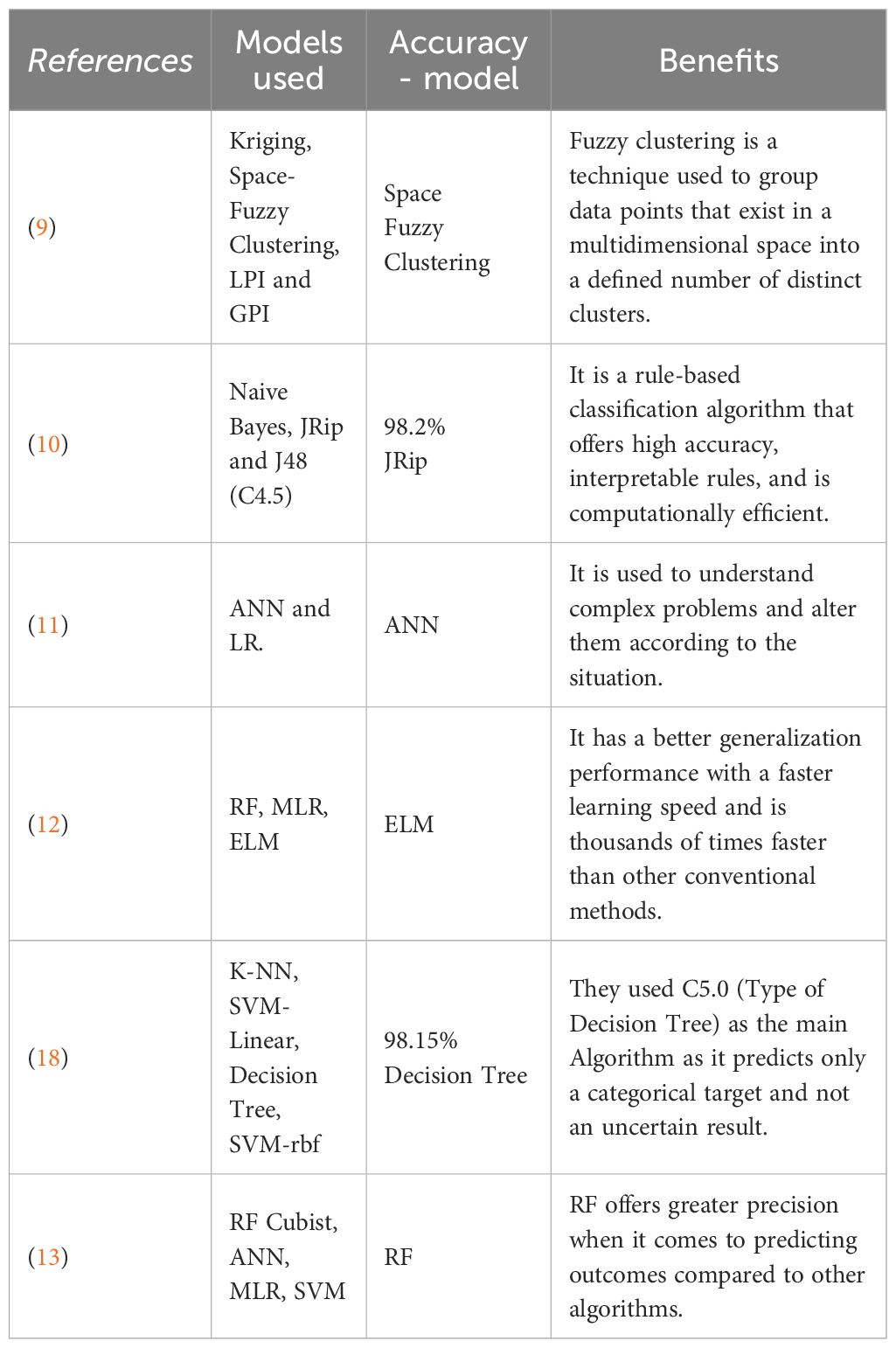
Table 1. Result of the proposed methods.

3 Proposed methodology

To assess the significance of the regression model, several Goodness of Fit (GOOF) parameters are computed, including the r-squared (R²) as shown in Equation 1, Lin’s concordance correlation coefficient (CCC) as shown in Equation 2, and RMSE as shown in Equation 3.

$\begin{array}{ll}{R}^2 = 1 - \frac{sum squared regression (SSR)}{total sum of squares (SST)} = 1 -\frac{{{\displaystyle \sum }}_{i=1}^N{(y_i-{\widehat{y}}_i)}^2}{{{\displaystyle \sum }}_{i=1}^N{(y_i-\underset{\_}{y})}^2}& (1)\end{array}$

$\begin{array}{ll}CCC = \frac{2\rho {\sigma }_{predicted}{\sigma }_{observed}}{{{\sigma }_{predicted}}^2+{{\sigma }_{observed}}^2+{({\mu }_{predicted}-{\mu }_{observed})}^2}& (2)\end{array}$

$\begin{array}{ll}RMSE = \sqrt[2]{\frac{{{\displaystyle \sum }}_{i=1}^N{(y_i-{\widehat{y}}_i)}^2}{N}}& (3)\end{array}$

where,

$y_i$= Actual Value,

${\widehat{y}}_i$ = Predicted Value,

$\underset{\_}{y}$ = Mean of the Actual Value,

ρ = correlation coefficient between variables ${\widehat{y}}_i$ and $y_i$

${\mu }_{predicted } , {\mu }_{observed }$ are the corresponding means

${\sigma }_{predicted},{\sigma }_{observed}$ are the corresponding variances of ${\widehat{y}}_i$ and $y_i$

The degree of variation is described by the coefficient of variation, whose size is measured; a coefficient of variation below 10% is regarded as having mild variability. one greater than 10% and less than or equal to 100% is considered to have moderate variability; and one greater than 100% is considered to have strong variability.

3.1 Dataset collection and preprocessing

Based on the dataset (22), it’s evident that the soil is abundantly enriched with all the necessary nutrients in quantities that surpass their respective threshold values. Upon examining the data, it can be concluded that the soil contains very little Cu, but adequate amounts of Macro nutrients, along with appropriate pH and EC levels. Additionally, the skewness values of Zn and OC indicate that the variables’ distribution is asymmetrical, while the kurtosis values of Cu and EC suggest that their distribution is uniform. The Standard Deviation of K indicates that its data is distributed throughout. The selected data is a multi-class i.e., three class datasets, which has the following properties (Table 2).

Table 2

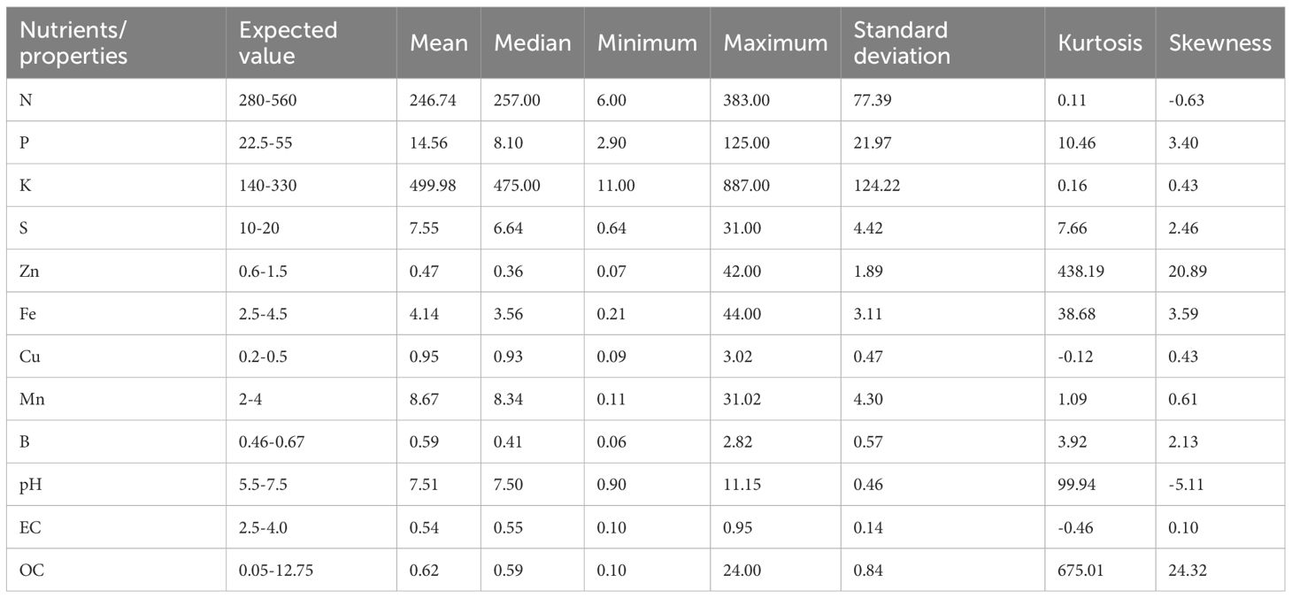
Table 2. Data interpretations.

Table 3 shows the summary of the soil fertility dataset, including basic structure, class distribution and preprocessing techniques applied. The dataset comprises 1980 samples with 12 features, including pH, N, P, K, EC, Zn, Fe, Cu, Mn, B, S, and Organic Carbon. The target variable represents soil fertility classified into three classes: Low (29%), Medium (45%), and High (26%). As the classes were moderately imbalanced, we employed SMOTE (Synthetic Minority Oversampling Technique) to balance the dataset before training. All models were evaluated using stratified 5-fold cross-validation to ensure fair representation of each class.

Table 3

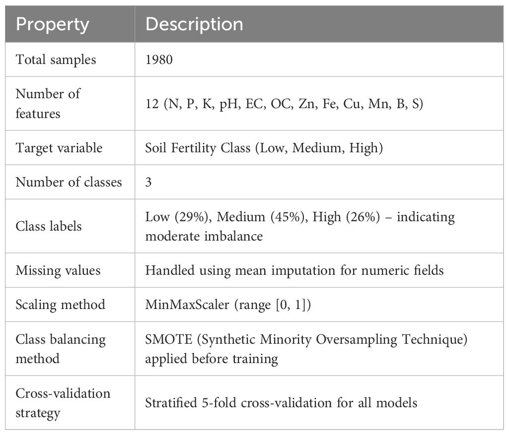
Table 3. Summary of the soil fertility dataset, including basic structure, class distribution and preprocessing techniques applied.

The preprocessing steps involves loading the data into a panda DataFrame, checking for and handling missing values and ensuring each column has the correct data type. Duplicates are checked and removed to avoid redundancy, and numerical features are scaled.

The preprocessing steps for the dataset included several stages to ensure data quality and consistency before model training. First, the dataset was loaded into a Pandas DataFrame, and all missing values were checked. Since a small number of entries had missing values, we used mean imputation for numerical fields such as nitrogen, phosphorus, and potassium. No categorical features were present in the dataset. Duplicate records were removed to prevent redundancy. All numerical features were then normalized using the MinMaxScaler, transforming values to the range [0, 1] to improve the convergence speed and stability of machine learning algorithms.

In addition, we performed correlation analysis to detect multicollinearity. Highly correlated features (correlation > 0.9) were reviewed, but none were removed since all parameters (e.g., N, P, K, pH, OC) had known agricultural significance. No synthetic features were added, but during model interpretation, feature importance techniques were applied (as discussed later). This preprocessing pipeline was consistently applied to both classical ML models and deep learning pipelines to ensure comparability.

The observed feature rankings are consistent where N, P, K, and pH were highlighted as the top contributors to fertility status in Indian agro-climatic zones. However, unlike previous works that used limited ML techniques or lab-processed datasets, our study integrates real-time sensor data, prototype hardware, and deep learning (LSTM, MLP) for prediction. Furthermore, our analysis goes beyond prediction by providing field-deployable insights via the AI-SISFMA kit and web/mobile dashboards—bridging the gap between lab research and agricultural field utility.

3.2 Models selection

To ensure a comprehensive evaluation and identify the most suitable algorithm for real-time soil fertility prediction, we implemented and compared 13 diverse machine learning and deep learning models. These algorithms were selected to represent a broad spectrum of learning paradigms, including: Ensemble-based models (Random Forest, XGBoost, Gradient Boosting, AdaBoost) for their ability to handle complex feature interactions and reduce overfitting. Linear models (Logistic Regression, Ridge Classifier) for their interpretability and baseline comparison. Support Vector Machines (SVM) for capturing nonlinear relationships with kernel tricks. K-Nearest Neighbors (KNN) as a non-parametric, distance-based method suitable for smaller datasets. Naïve Bayes for its speed and probabilistic nature. Decision Trees for simplicity and interpretability. Multi-Layer Perceptron (MLP) and Long Short-Term Memory (LSTM) (38) networks to assess deep learning effectiveness on structured tabular data. This diversity allowed us to benchmark performance across different algorithmic families, minimize bias from model selection, and identify which approaches generalize best in the context of imbalanced, real-world agricultural datasets. Ultimately, the top-performing models were retained for further analysis and deployment in the SISFMA system.

3.2.1 Random forest classifier

The RF Classifier is an ensemble learning algorithm that is utilized for classification tasks. Its basic idea is to build a collection of decision trees, each of them is trained using a different subset of the training features and data. This method lessens overfitting and improves precision. Because each tree concentrates on a distinct subset of the data and characteristics, this helps to increase generalization performance and lessen overfitting. RF Classifier (6) can be expressed as in Equation 4:

$\begin{array}{ll}y = mode \left\{ f1(x), f2(x), \dots , fn(x) \right\}& (4)\end{array}$

where,

$y$ is the predicted class label,

$fi(x)$ is the predicted class label,

$n$ is the total number of decision trees in the forest.

This work builds upon earlier studies on soil fertility analysis (29) which demonstrated the benefit of ensemble classifiers in agricultural prediction. A RF classifier can be implemented to assign soil samples to fertility categories purely at random. It does this without learning from the features (such as chemical composition or texture). By comparing the performance of more sophisticated models to this random classifier, you can assess whether those models are genuinely useful. Ensure that performance comparison is done using techniques like k-fold cross-validation. This divides the dataset into training and testing sets, and average performance is used to avoid bias. A soil fertility classifier can be used for: Farmers can receive recommendations based on the fertility class of soil to decide on the appropriate type and quantity of fertilizers; Identifying areas of low fertility for targeted interventions, preventing further degradation of the soil; Agricultural Decision Support Systems (DSS): Incorporating classification models into tools that guide farmers and agronomists on sustainable land management practices.

3.2.2 ExtraTrees classifier

It comes under the supervision classifier and is an ensemble technique that deals with selecting a random decision tree method to design the model. Fertilizers are administered at random, and soil samples are tested in a lab to determine the levels of soil fertility. This conventional method pollutes the environment and raises fertilization prices. Therefore, it is essential to create a reliable and affordable classification system for soil fertility and fertilizer application. It is an extension of the RF algorithm, and like RF, it builds multiple decision trees and combines their predictions to obtain the final output. The splitting thresholds for the decision trees are selected randomly, rather than based on a measure of impurity such as Gini or entropy. ExtraTrees doesn’t rely on bootstrap sampling (random subsets of data with replacement) as Random Forest does. It uses the whole dataset for each tree, but adds randomness by splitting the nodes. The ExtraTrees Classifier can be very effective in soil fertility classification tasks. Soil datasets often include numerous features (e.g., nitrogen content, moisture, pH levels). ExtraTrees handles high-dimensional data well by focusing only on random subsets of features when splitting nodes. The relationship between soil properties and fertility is often non-linear. ExtraTrees, like other tree-based algorithms, can capture such non-linear interactions between soil properties effectively. ExtraTrees provide a natural way to measure feature importance, allowing you to determine which soil characteristics (e.g., organic matter, pH, moisture) are most predictive of fertility levels. A real-world case study was incorporated using ExtraTrees Classifier (23).

3.2.3 Stochastic gradient descent classifier

SGD Classifier is a type of linear classifier used for binary and multiclass classification tasks in ML. It is a simple and efficient algorithm that updates the model parameters iteratively, based on the gradients of the loss function with respect to the parameters. The Equation 5 for the SGD Classifier can be expressed as follows:

$\begin{array}{ll}w(t+1) = w(t) - eta * grad(Loss(w(t), xi, yi))& (5)\end{array}$

where,

$w(t)$ is the weight vector at iteration $t$,

$eta$ is the learning,

$grad(Loss(w(t), xi, yi))$ is the loss function’s gradient,

$Loss(w(t), xi, yi))$ is the loss function.

In this study, the authors employed ML classifiers, including SGD, to classify soil samples based on fertility levels. They found that SGD Classifier, when combined with feature scaling and data preprocessing, performed efficiently in classifying large soil datasets. The study highlights the effectiveness of SGD in handling real-world agricultural datasets, especially where scalability is critical. This article demonstrates how SGD can be applied in practical soil fertility analysis, addressing computational efficiency and accuracy in predicting soil classes. The research emphasized using spectral data from soil samples to improve prediction performance in machine learning applications.

3.2.4 Support vector machine

The algorithm is widely utilized in machine learning for both binary and multi-class classification tasks due to its effectiveness. Its objective is to determine the hyperplane that optimally separates the data points into distinct classes, with a focus on maximizing the margin between the hyperplane and the nearest data points (known as the support vectors). The equation for the SVM algorithm can be expressed as follows in Equation 6:

$\begin{array}{ll}y(x) = sgm (wT \times x + b)& (6)\end{array}$

where,

$y(x)$ is the predicted class label for the input sample $x$,

$w$ is the weight vector that defines the orientation of the hyperplane,

$b$ is the bias term that shifts the hyperplane away from the origin.

In this study, the researchers employed SVM (24) to classify soil fertility levels based on both laboratory soil data and remote sensing information. The use of SVM with an RBF kernel was highlighted due to its ability to capture non-linear relationships in the data, leading to high classification accuracy. The study found that SVM outperformed other classifiers when dealing with complex and multi-dimensional soil datasets, particularly when combined with feature scaling and cross-validation techniques. This article illustrates the effectiveness of SVM in soil fertility analysis, emphasizing its potential for remote sensing applications, where large-scale soil data can be integrated into the model. It also underscores SVM’s strength in handling both linear and non-linear data relationships in agricultural datasets.

3.2.5 Logistic regression

It is a popular algorithm used for binary classification tasks in machine learning. It models the probability of a binary response variable (i.e., the presence or absence of a certain outcome) as a function of one or more predictor variables (i.e., features), using a logistic or sigmoid function. The expression for logistic regression, represented in Equation 7, can be stated in the following manner.

$\begin{array}{ll}p(y=\frac{1}{x})=e^z& (7)\end{array}$

where,

$z = (w^T \text{x }+\text{ b})$, $p(y=\frac{1}{x})$ is the conditional probability of the positive class (i.e., $y=1$) given the input features,

$x$, $z$ is a linear combination of the input features and the model parameters (weights and bias).

In this study, Logistic Regression (25) was applied to predict soil fertility classes based on physicochemical properties such as pH, nitrogen, phosphorus, and organic carbon content. The authors highlighted the interpretability of Logistic Regression and demonstrated that the model provided reliable predictions while identifying the most significant features influencing fertility. They also emphasized the importance of feature scaling and cross-validation to improve model performance and generalization. This article illustrates the practical application of Logistic Regression in soil fertility analysis, showing that despite its simplicity compared to more complex models, Logistic Regression can offer accurate and interpretable results, making it a suitable choice for agricultural data analysis.

3.2.6 Ridge classifier

The Ridge Classifier is a form of linear classifier that shares similarities with logistic regression. However, it utilizes L2 regularization to prevent overfitting and enhance generalization performance. Its primary objective is to locate the linear function that most effectively divides the data points into distinct categories, while minimizing the sum of squared weights. The Ridge Classifier can be considered a middle ground between the L1 regularization-based linear SVM and the non-regularized logistic regression. It is especially beneficial when dealing with correlated and high-dimensional data as L2 regularization can stabilize the weights and decrease overfitting.

This study examined the effectiveness of regularized classification models, including Ridge Classifier, in predicting soil fertility levels. The research found that Ridge Classifier (26) performed well in handling the multicollinearity present in soil datasets and provided more stable predictions compared to non-regularized models. The Ridge Classifier’s ability to shrink coefficients resulted in improved generalization and interpretation of the influential soil properties. The authors emphasized the importance of regularization for ensuring model robustness, particularly in agricultural datasets prone to overfitting. This article illustrates how Ridge Classifier can be used to enhance the organization of soil fertility, demonstrating the advantages of regularization in agricultural data analysis.

3.2.7 KNeighbors classifier

The KNeighbors Classifier algorithm is widely utilized in machine learning for classification tasks. This algorithm is categorized as an instance-based or lazy learning method, which predicts the output class of a new sample based on the majority vote of its K-Nearest Neighbor in the training data, utilizing a specific distance metric. The algorithm involves two primary steps: first, computing the distance between the input sample and selecting the K-nearest Neighbor, and second, aggregating their class labels to make a prediction. In this study, the authors applied the KNN (27) algorithm to predict soil fertility classes based on soil properties. The study demonstrated that KNN achieved high accuracy in classifying soil fertility, particularly when combined with feature scaling and cross-validation. The authors also emphasized the importance of selecting an appropriate “k” value to optimize the model’s performance. The research highlighted the simplicity and effectiveness of KNN for soil fertility prediction in precision agriculture. This article provides a comprehensive exploration of how KNN can be applied in real-world soil fertility analysis, illustrating its usefulness in predicting soil health and supporting decision-making in agriculture.

3.2.8 Gradient boosting classifier

The described classifier is an ensemble learning technique (28) that amalgamates several weak learners to generate a robust predictive model. The method operates by progressively including fresh decision trees into the model, where every tree is trained to rectify the mistakes made by the preceding one. The ultimate forecast is derived by accumulating the projections of all the trees. Mathematically, the prediction of the Gradient Boosting Classifier can be represented by the following Equation 8:

$\begin{array}{ll}F(x) = {\displaystyle \sum }_{m=1}^M\eta (x) H_m(x) & (8)\end{array}$

where,

$F(x)$ is the final prediction,

η is the learning rate,

$H_m(x)$ is the prediction of the $m$ ^th decision tree,

$M$ is the total number of trees.

In this study, the authors employed Gradient Boosting Classifier (29) to predict soil fertility based on soil properties. They found that Gradient Boosting outperformed other classifiers like RF and LR, particularly in capturing non-linear interactions between soil properties. The model’s ability to identify the most significant factors in soil fertility helped inform better agricultural practices and fertilizer management strategies. The study also discussed how hyperparameter tuning and regularization helped improve model performance and prevent overfitting. This research highlights the advantages of Gradient Boosting in dealing with complex agricultural data and showcases its effectiveness in making accurate soil fertility predictions.

3.2.9 AdaBoost

It is a boosting algorithm (30) that syndicates weak classifiers into a strong classifier. It assigns weights to training examples based on their classification error and trains a sequence of weak classifiers on weighted training data. The final classification is determined by a weighted combination of the weak classifiers. The Formula 9 for the AdaBoost classifier is:

$\begin{array}{ll}H(x) = sgm({\displaystyle \sum }_{t=1}^T{\alpha }_t{H}_t(x) )& (9)\end{array}$

where,

$H_t(x)$ is the final classifier,

${\alpha }_t$ is the weight assigned,

$T$ is the number of weak classifiers.

3.2.10 Fuzzy c-means

It is a clustering algorithm that assigns each data point a membership grade for each cluster, allowing it to handle uncertain or overlapping data. It iteratively updates the cluster centers and membership grades until convergence. The Formula 10 for fuzzy c-means is:

$\begin{array}{ll}J={\displaystyle {\sum }_{i=1}^N{\displaystyle {\sum }_{j=1}^{C}w{(i,j)}^m{(x(i)-\text{µ}(j))}^2}}& (10)\end{array}$

$\begin{array}{ll}w(i,j)={\displaystyle {\sum }_{k=1}^C\frac{(x(i)-\text{µ}(j))}{{(x(i)-\mu (k))}^{{(\frac{2}{(m-1)})}^{-1}}}}& (11)\end{array}$

$\begin{array}{ll}\text{µ}(j)=\frac{{{\displaystyle \sum }}_{i=1}^{N}w{(i,j)}^{m}x(i)}{{{\displaystyle \sum }}_{i=1}^{N}w{(i,j)}^m}& (12)\end{array}$

where,

$J$ (Equation 11) is the objective function to be minimized,

$w(i,j)$ (Equation 11) is the membership grade of data point

$i$ in cluster $j$,

$m$ is a weighting exponent,

$x(i)$ is the $i$^th data point,

$\mu (j)$ (Equation 12) is the centroid of cluster $j$,

$N$ is the number of data points,

$C$ is the number of clusters.

3.2.11 Decision tree classifier

The algorithm utilized in machine learning is known as a decision tree model. This model is structured as a tree, which contains various decisions and their potential outcomes. The algorithm partitions data recursively according to the values of features, and at each split, it selects the feature that offers the most information gain. The Equation 13 for the decision tree classifier is:

$\begin{array}{ll}H(x) = argmax ({\displaystyle {\sum }_{t=1}^T[y_i = c] p(i | x)} )& (13)\end{array}$

where H(x) is the predicted class for input x, c is the class label, y_i is the i-th training instance, N is the number of instances, and p(i | x) is the probability of the instance i given input x.

3.2.12 The perceptron

It is a binary classification algorithm that learns a linear decision boundary to separate data points. It computes the weighted sum of input features and applies a threshold function to make a prediction. The weights and bias are updated based on the classification error at each iteration. Equation 14 for the perceptron is:

$\begin{array}{ll}H(x) = sign(w·x + b)& (14)\end{array}$

where H(x) = the predicted class for input x, w = the weight vector, ‘·’ denotes the dot product and b is the bias term. The Perceptron model (31–33) can be trained using labelled soil data to classify soil samples based on fertility levels. Key soil parameters such as pH, nutrient levels (N, P,K), organic matter, and texture can serve as inputs, while the fertility category (e.g., low, medium, high) is the output. The Perceptron adjusts its weights to learn the relationship between input features and soil fertility status, allowing for the prediction of soil fertility for new, unseen data.

3.2.13 K-means

The given content describes an unsupervised clustering technique that separates n data points into k clusters. Initially, k centroids are randomly selected, and each data point is assigned to the closest centroid. Then, the centroid of each cluster is recalculated by taking the mean of the points in that cluster. The algorithm continuously updates the cluster assignments and centroids until it reaches convergence. The ultimate outcome is k clusters that group together the data points with similar distances to their respective centroid.

K-means (34) can group soil samples into clusters based on their chemical and physical properties. This helps researchers identify patterns in soil fertility across different regions, guiding crop selection and soil management practices. For instance, clustering can reveal zones that are nutrient-rich versus those that are nutrient-poor. In precision agriculture, K-means is used to delineate management zones in a field based on fertility indicators like nitrogen, phosphorus, or organic carbon content. These clusters enable more targeted interventions, such as adjusting fertilizer application rates to specific areas rather than treating the entire field uniformly. The technique allows for spatial mapping of soil variability, offering insights into soil fertility distribution. These clusters are used to create soil maps that visually represent the variation of soil characteristics (35, 36) within a specific area, helping optimize land management decisions. Soil datasets often include many overlapping variables. K-means simplifies the interpretation by clustering similar data points together, making it easier to identify distinct soil types or conditions that influence plant growth.

3.3 Deep learning algorithms

The proposed work also predicts the type of crop that can be grown in the given area. The prediction is done using deep learning techniques.

3.3.1 Multi-layer perceptron

MLPs (37) are particularly well-suited for tabular data where features (e.g., soil type, pH, temperature) are independent but still collectively influence the output. Unlike CNNs (used for images) or RNNs (used for sequences), MLPs effectively model relationships in structured data. Crop recommendation is a non-linear problem where features interact in complex ways (e.g., high pH combined with low temperature favors one crop but not another). MLP, with its hidden layers and activation functions, can learn such relationships.

Unlike image data where spatial relationships are important (handled by CNNs), or sequential data where order matters (handled by RNNs), MLPs treat each input feature independently, making them ideal for datasets like this. The following are the layers inside the MLP.

3.3.1.1 Input layer

The input layer takes in all the features from the dataset, such as soil type, temperature, humidity, and other relevant parameters. This layer acts as a gateway to feed structured/tabular data into the neural network. Each feature is assigned to a neuron, and no processing occurs here—it simply passes the raw data to the next layer.

3.3.1.2 Hidden layers

Hidden layers are the heart of the MLP, where the model learns relationships and patterns in the data.

a. First Hidden Layer: This layer begins to extract underlying relationships between the features. For example, it may combine the temperature and humidity features to understand how they jointly influence crop suitability. ReLU (Rectified Linear Unit) activation is applied to ensure the model can capture complex, non-linear relationships in the data.

b. Second Hidden Layer: This layer refines the patterns learned from the first hidden layer. For instance, it might distinguish between crops that thrive in wet soils versus those suited for dry conditions. The smaller number of neurons compared to the first layer ensures the model progressively simplifies and narrows down important patterns.

c. Third Hidden Layer: The model further condenses the extracted information, focusing only on the most critical features and relationships that help differentiate between crop recommendations.

3.3.1.3 Dropout layers

Dropout is a regularization technique added after some hidden layers to prevent overfitting. It temporarily deactivates a random subset of neurons during training, forcing the model to rely on a broader set of features rather than memorizing the training data. This improves the model’s generalizability to unseen data.

3.3.1.4 Output layer

The final layer provides the predicted probabilities for each class (crop type). A softmax activation function is used here, ensuring the output represents probabilities across all possible crops. The crop with the highest probability is chosen as the recommendation.

Table 4 shows the architecture of the MLP model. It consisted of an input layer with 12 neurons (corresponding to the 12 features), followed by three hidden layers with 64, 32, and 16 neurons respectively. The activation function used in all hidden layers was ReLU, and Dropout of 0.3 was applied after each hidden layer to prevent overfitting. The output layer used a Softmax activation function for multi-class classification. The model was trained using the Adam optimizer with a learning rate of 0.001, a batch size of 32, and for 50 epochs. Categorical cross-entropy was used as the loss function. Early stopping with a patience of 5 epochs was applied based on validation loss.

Table 4

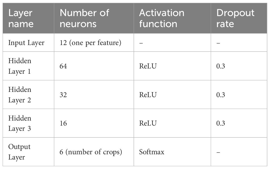
Table 4. Architecture of the multi-layer perceptron (MLP) model.

3.3.2 Long short-term memory

A robust neural network architecture integrates several key components to enhance its performance and versatility. A Bidirectional LSTM captures patterns from both past and future contexts, enabling richer feature representation, while a Stacked LSTM deepens the ability to learn complex temporal patterns within sequences. Dense layers (MLP) further refine these sequential features, transforming them into compact representations suitable for classification tasks. Dropout is employed to mitigate overfitting by randomly deactivating neurons during training, ensuring a more generalized model. Finally, a Softmax layer converts the network’s outputs into a probability distribution, facilitating effective multi-class classification. LSTMs excel at learning sequential patterns, long-term dependencies, and temporal relationships in data, addressing challenges that static models like MLPs cannot handle effectively on their own. While LSTMs capture the sequential features, MLPs play a complementary role by transforming these features and facilitating classification. This combination adds flexibility to the model and enables the learning of non-linear decision boundaries, enhancing overall performance.

Table 5 shows the architecture of LSTM model. The hybrid model used a Bidirectional LSTM layer with 64 units, followed by a Dropout layer (0.2) and two Dense layers with 32 and 16 neurons respectively. The final output layer used Softmax activation for multi-class classification. This model was also trained using Adam optimizer with a learning rate of 0.001, a batch size of 64, and for 50 epochs. The model was validated using an 80:10:10 split (train:val:test) and monitored using early stopping.

Table 5

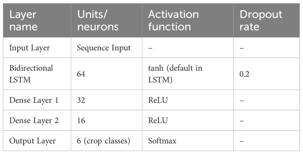
Table 5. Architecture of the LSTM model.

3.3.3 Training strategies and overfitting control

During the training of deep learning models (MLP and LSTM), early stopping was implemented to prevent overfitting. The training process was monitored using validation loss, and training was halted if no improvement was observed for 5 consecutive epochs. A fixed learning rate of 0.001 was used throughout training; learning rate scheduling techniques were not applied in this study to keep the training process consistent across models. Since the dataset consists of structured tabular data, data augmentation techniques were not applicable and were therefore not used.

3.4 Experimental analysis using ML algorithms

3.4.1 Hyperparameter tuning

The potential of the Ensemble models is also enhanced to the maximum possible extent by utilizing the ‘RandomizedSearchCV’ function, which is a part of the ‘model_selection’ module in the ‘scikit’ library. This function performs a search through the given hyperparameters distribution to identify the optimal values for the model. In addition, a 7-fold cross-validation scheme (cv=7) is used to improve the accuracy of the model. After fitting the training data into the model, the best parameters are extracted from the results obtained from the Randomized Search to ensure the model is fine-tuned to its highest potential.

3.4.2 Evaluation metrics and results

With the fully optimized Random Tree model, it has been concluded that prediction of soil fertility is possible with a splendid maximum accuracy of 92.42%. Along with the highest accuracy model, added the other model’s accuracy, precision, and recall values (Table 6). The percentage of correct predictions out of all predictions. Higher accuracy indicates better performance. The RF classifier has the highest accuracy (92.42%). Precision is the proportion of positive predictions that are actually correct. ExtraTrees Classifier has the highest precision (78.23% and good at identifying true positives without many false positives. A higher F1 score indicates a better balance between precision and recall. Gradient Boosting Classifier has the highest F1 score (70.92%). The Gradient Boosting Classifier has the highest recall (71.26%), and identifies the true positives.

Table 6

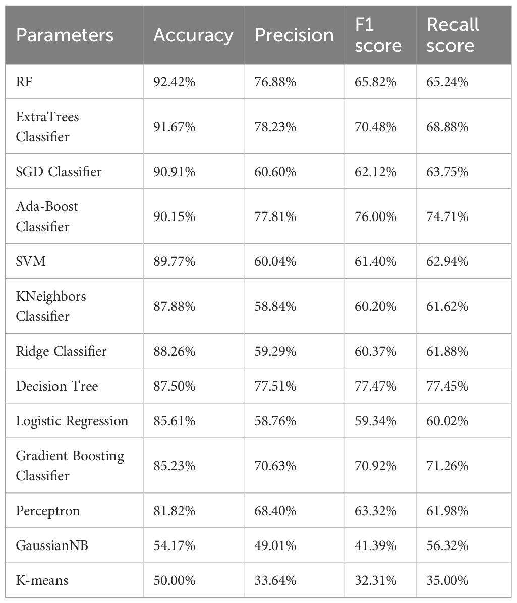
Table 6. Prediction results of ML models.

Later comes the comparison, through a bar graph, of the Accuracy, precision, and Recall score calculated applying the equation no: (15), (16) and (17), respectively of all the algorithms in a detailed manner.

$\begin{array}{ll}Accuracy = \frac{Number of correct predictions}{Total number of true positives }& (15)\end{array}$

$\begin{array}{ll}Precisio{n}_{score}= \frac{TP}{TP + FP } & (16)\end{array}$

$\begin{array}{ll}Recall Score = \frac{TP}{TP +FN} & (17)\end{array}$

Accuracy [depicted Figure 1] can be defined as the fraction of predictions the model got right and the agreement between a measured value and an accepted value. It can be calculated by dividing the number of correct predictions by Total number of true positives (TP).

Figure 1

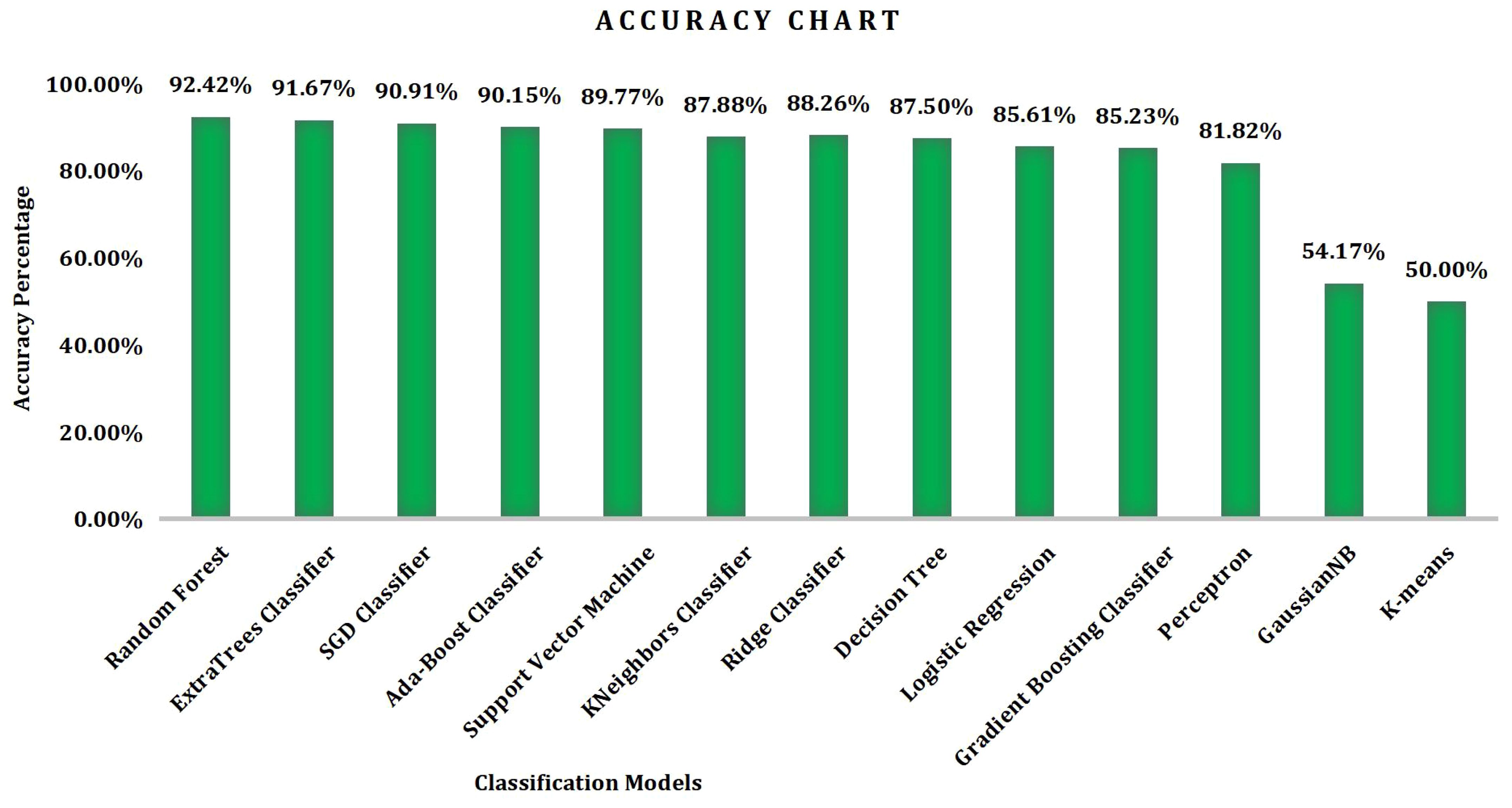
Figure 1. Accuracy graph obtained using ML algorithms.

Precision [shown in Figure 2] can be estimated by dividing TP by the sum of TP and the sum of false positives (FP) predictions.

Figure 2

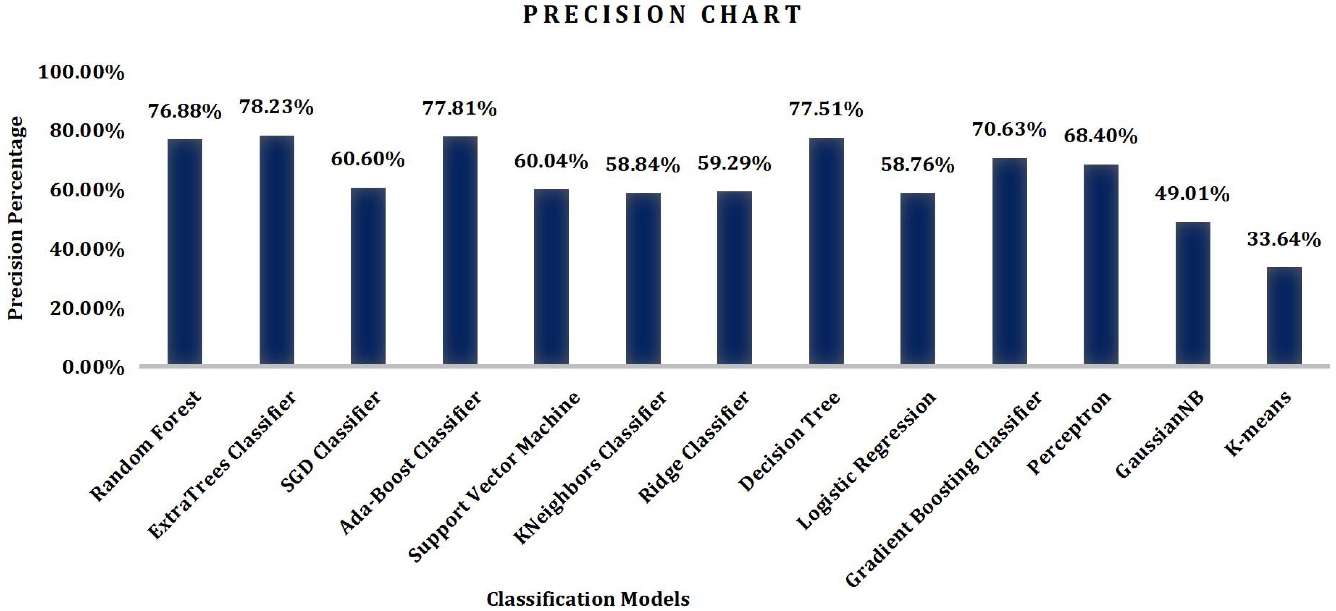
Figure 2. Precision graph obtained using ML algorithms.

Recall [refer Figure 3] can be calculated by dividing TP by the sum of TP and total number of false negatives (FN).

Figure 3

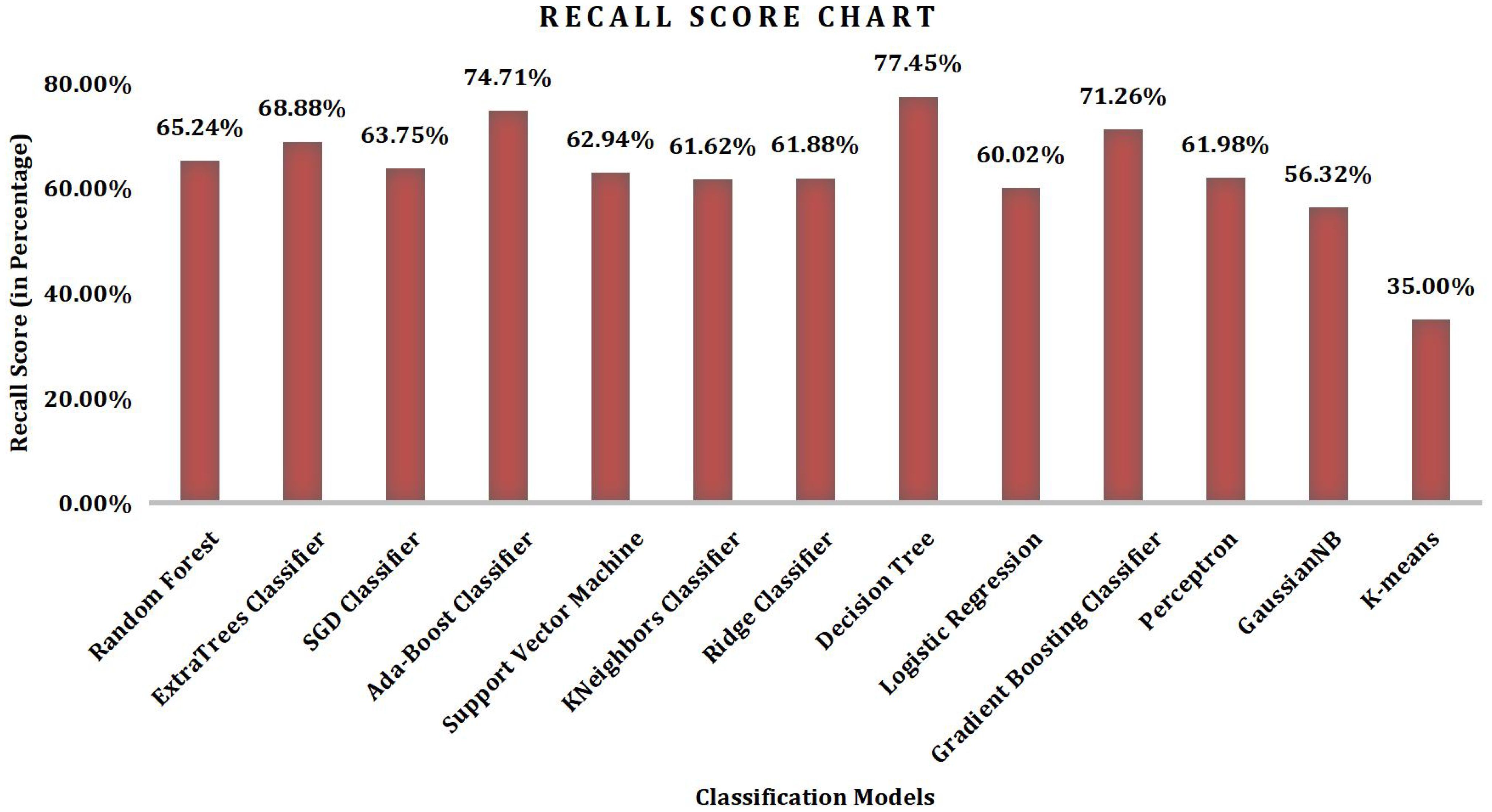
Figure 3. Recall graph obtained using ML algorithms.

Furthermore, it is possible to calculate the values of TP, Total number of True Negatives (TN), FP and FN using the Confusion Matrix (Table 7) obtained.

Table 7

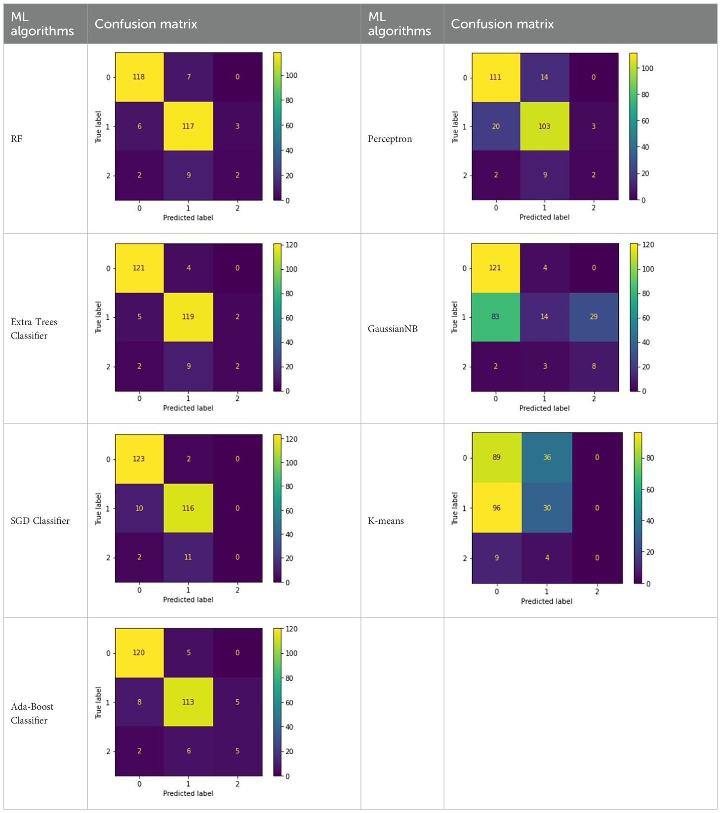
Table 7. Confusion Matrix obtained using ML algorithms (22).

While RF exhibited the highest overall accuracy (92.4%), its F1-score was lower compared to Gradient Boosting and XGBoost due to class imbalance effects. The latter models achieved better recall and F1-scores, especially for minority classes (Low and High fertility). This highlights that accuracy alone is not sufficient to assess performance in imbalanced classification tasks. Therefore, models were further compared using macro-average F1-scores and confusion matrices to assess class-wise prediction capability.

Among all models evaluated, RF and XGBoost outperformed others due to their robustness against overfitting, ability to handle nonlinear feature interactions, and inherent feature selection mechanisms. XGBoost, in particular, benefits from boosting weak learners and optimizing loss with regularization, which explains its superior F1-score and Recall across fertility classes. In contrast, models like SVM and Logistic Regression struggled to model nonlinear relationships present in the dataset.

3.4.3 Implementation With MLP

The Confusion matrix in Figure 4 shows that the most predictions align with the actual labels, as evidenced by the high values along the diagonal. For example, all instances of potato (20) and most instances of grapes (20/21) are correctly classified. However, there are a few misclassifications: 1 instance of grapes is classified as pomegranate, 1 mango as mulberry, 2 mulberries as ragi, and 1 pomegranate as grapes. This indicates that while the model performs well overall, there is slight confusion between certain classes, which might be addressed by improving feature differentiation or fine-tuning the model further.

Figure 4

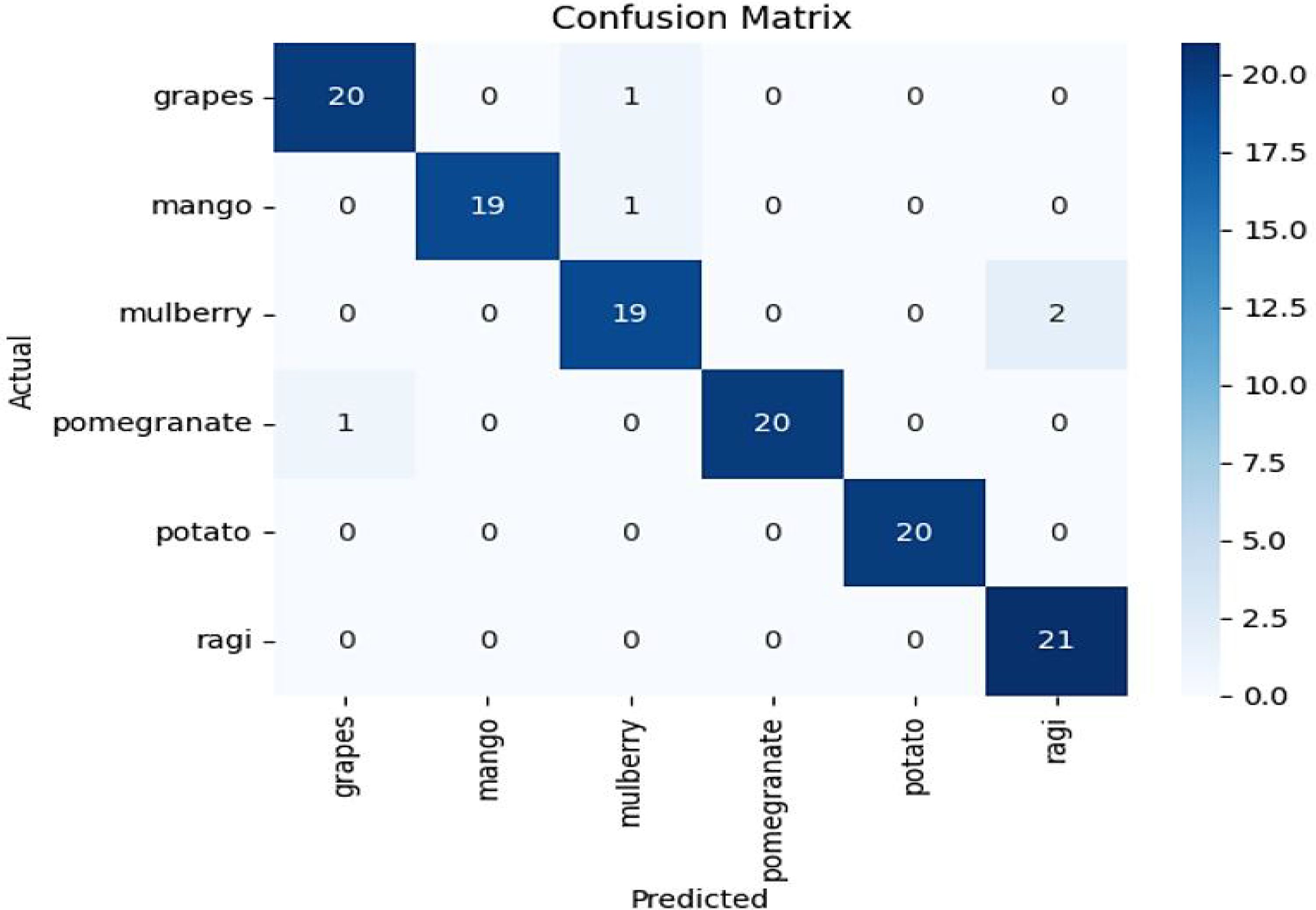
Figure 4. Confusion matrix for MLP model.

The confusion matrix for MLP shows accurate predictions for “Medium” and “High” classes, but noticeable confusion between “Low” and “Medium,” reflecting class overlap. This justifies the lower recall and F1-score for the “Low” class.

To ensure robust training and evaluation of the deep learning models, the dataset was split into three subsets: 80% for training, 10% for validation, and 10% for testing. The split was performed randomly but ensured class stratification to maintain the original distribution of soil fertility classes. The validation set was used for hyperparameter tuning and early stopping to prevent overfitting, while the final model performance was reported on the hold-out test set. Additionally, we averaged the performance over multiple random seeds to ensure consistency.

The classification report (Figure 5) shows that the model achieves an overall accuracy of 96%, with high precision, recall, and F1-scores across all classes. Mulberry, pomegranate, and potato have perfect precision and recall, indicating no false positives or false negatives for these classes. Grapes and mango also perform well with slightly lower scores, while ragi has the lowest precision (91%), suggesting some false positives for this class. Both macro and weighted averages for all metrics are consistently at 96%, indicating balanced performance regardless of class distribution. Overall, the model is robust and well-generalized, with minor room for improvement in ragi’s classification.

Figure 5

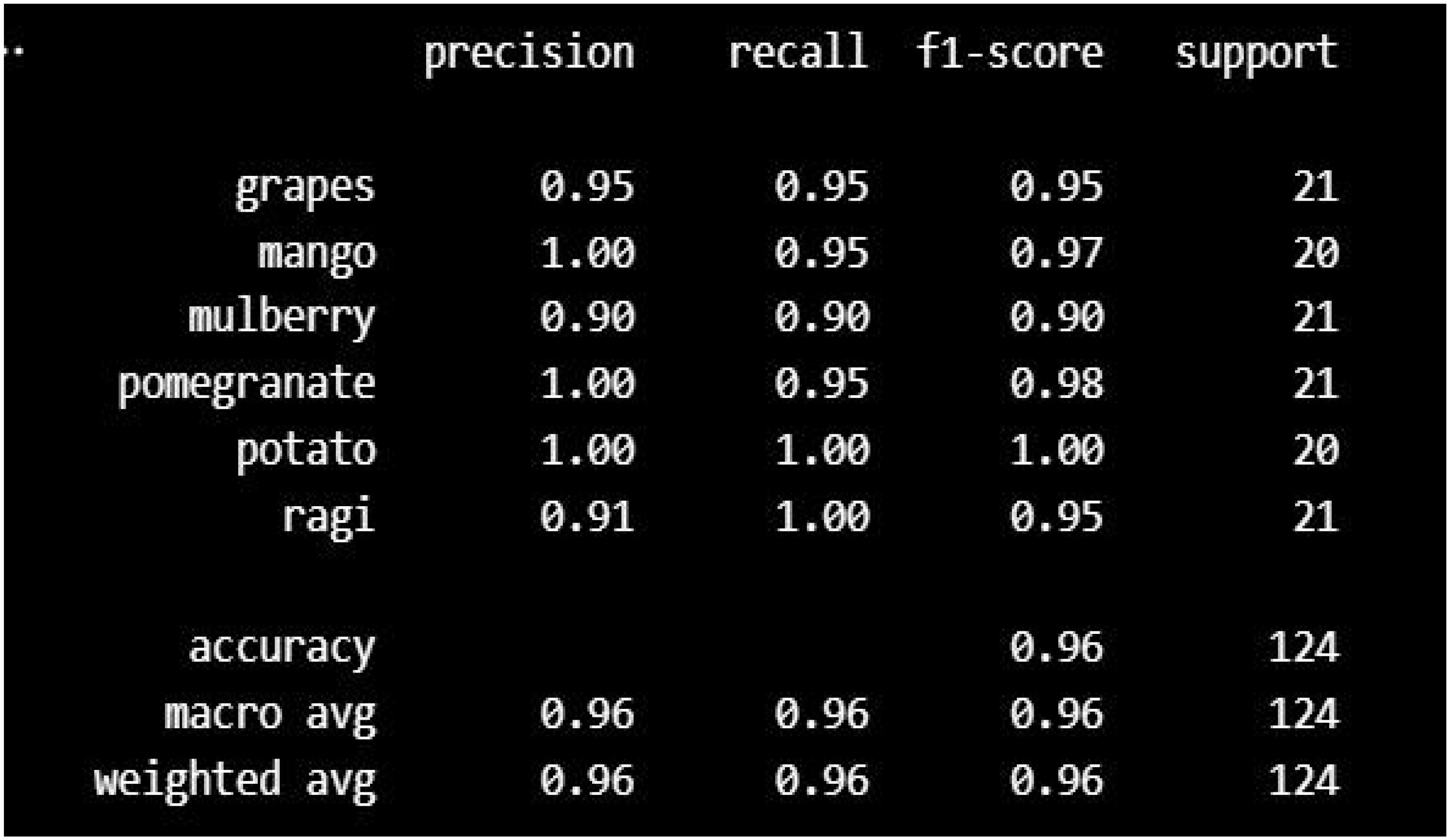
Figure 5. Performance metrics for MLP model.

The training and validation performance plots in Figure 6 indicate that the model learns effectively on the training data, as shown by the steadily decreasing training loss and increasing training accuracy, which stabilizes near 1.0. However, the validation loss initially decreases but then starts increasing, while the validation accuracy plateaus below the training accuracy, highlighting overfitting. This suggests that while the model performs well on the training data, its generalization to unseen data deteriorates over time.

Figure 6

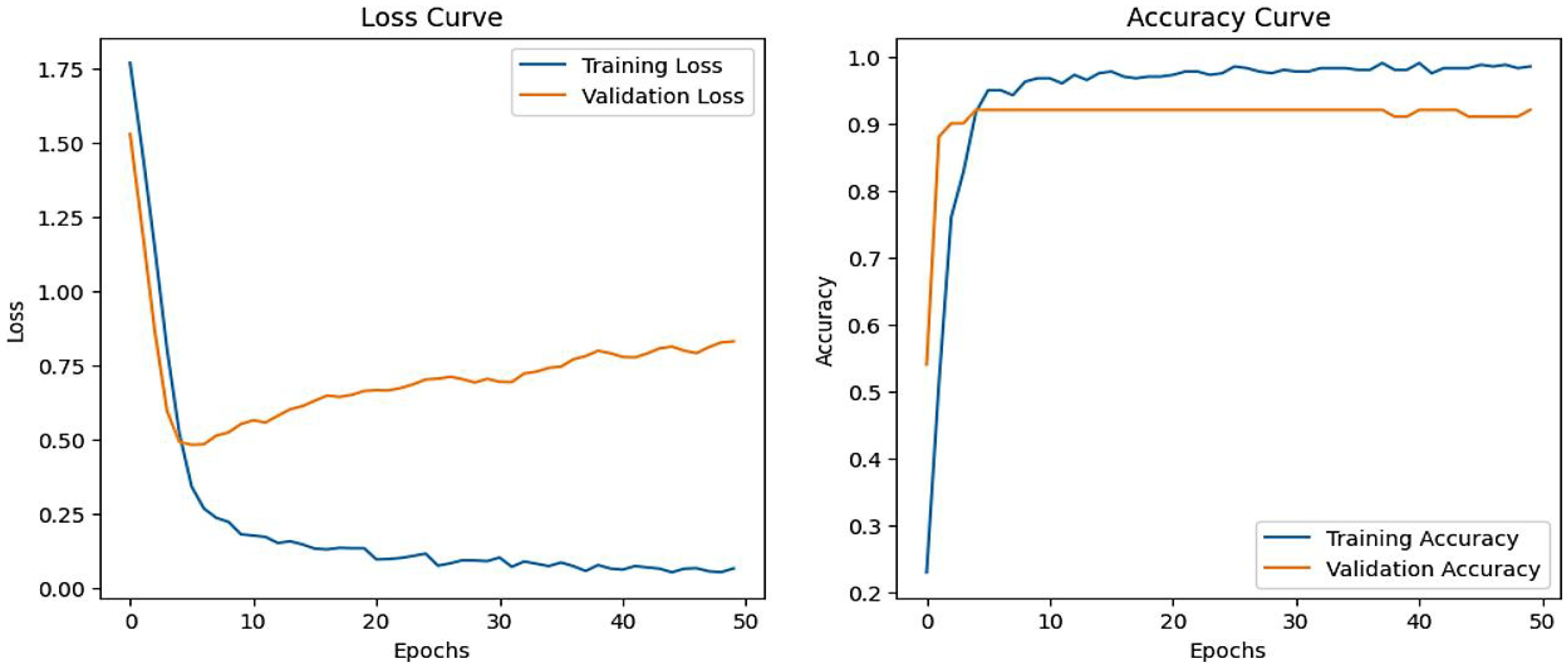
Figure 6. Accuracy, loss vs epochs curve for MLP model.

The confusion matrix in Figure 7 shows that majority of predictions are correct, as indicated by the dominant diagonal values. For instance, all mulberry (21), most grapes (23/24), pomegranate (21/22), potato (22/23), and ragi (16/17) instances are correctly classified. However, some misclassifications are observed: 1 grape is classified as ragi, 1 mango as grape, 1 pomegranate as mango, and 1 potato as ragi. These misclassifications suggest that while the model generally performs well, certain class boundaries might overlap, which could be addressed by refining the model or incorporating additional distinguishing features.

Figure 7

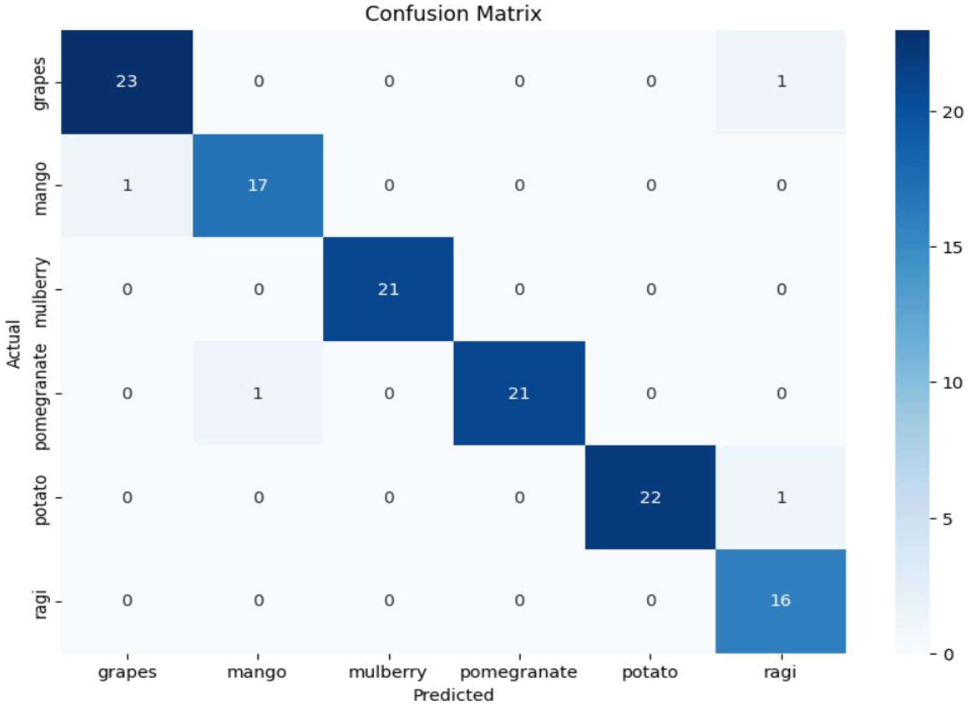
Figure 7. Confusion matrix for hybrid model (MLP WITH LSTM).

The classification report (Figure 8) indicates that the model performs exceptionally well, achieving an overall accuracy of 97% with high precision, recall, and F1-scores across most classes. Classes such as mulberry and pomegranate show near-perfect performance, while ragi has the lowest precision (89%), indicating some false positives for this class. Despite minor variations, the weighted average metrics confirm consistent performance, with the model handling class imbalances effectively. Overall, the model is highly reliable, but slight improvements could be made for specific classes like ragi to enhance precision.

Figure 8

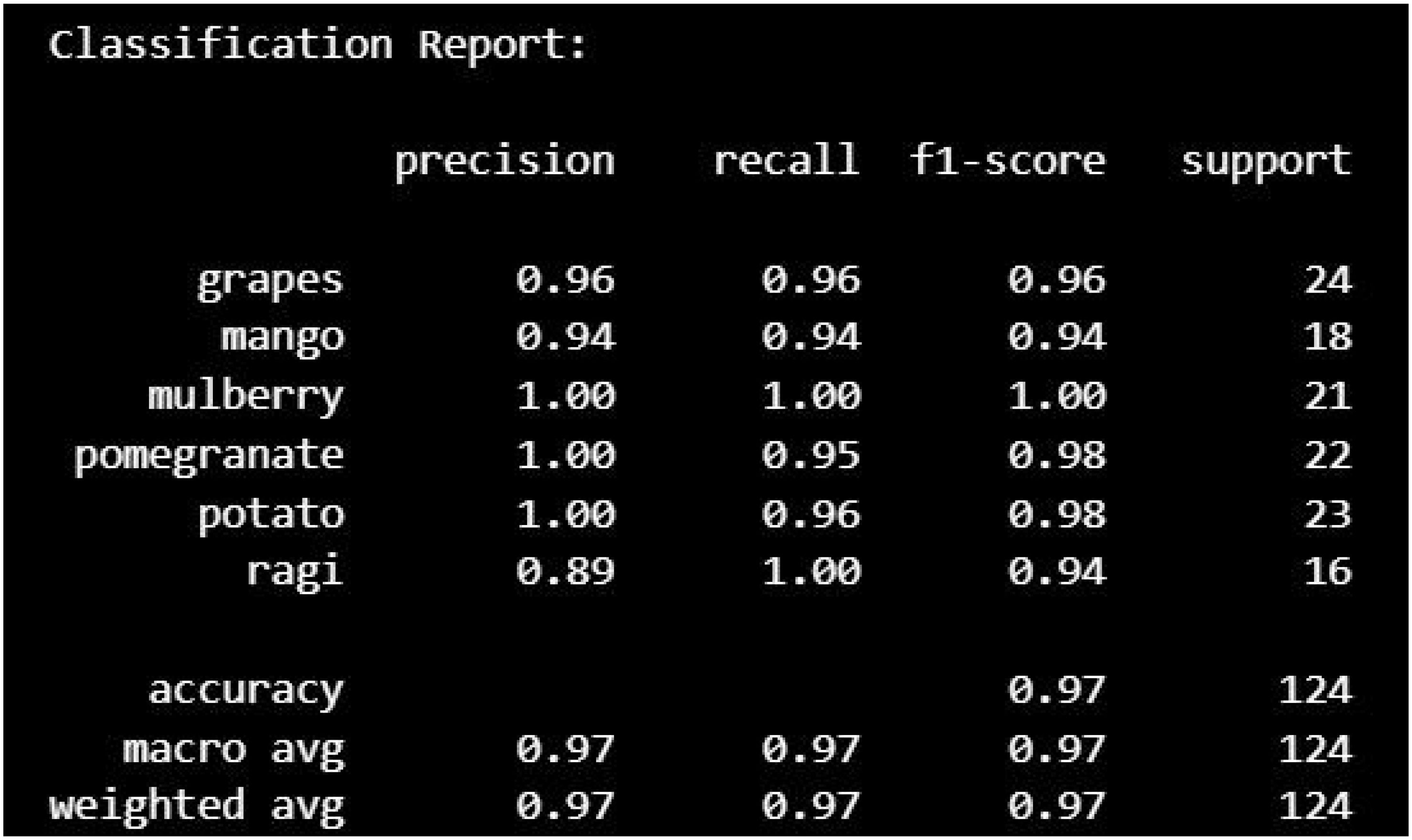
Figure 8. Performance metrics for hybrid model (MLP WITH LSTM).

The graphs (Figure 9) show the accuracy and loss trends of the Hybrid model (MLP with LSTM) over 50 epochs. The accuracy curve (left) indicates steady improvement in both training and validation accuracy, with the model reaching near convergence after approximately 20 epochs. Training and validation accuracy closely align, suggesting minimal overfitting and a well-generalized model. The loss curve (right) shows a rapid decrease in both training and validation loss during the initial epochs, eventually stabilizing as the model learns. The validation loss aligns well with training loss, further confirming the absence of significant overfitting. Overall, the model demonstrates effective training and generalization with consistent performance.

Figure 9

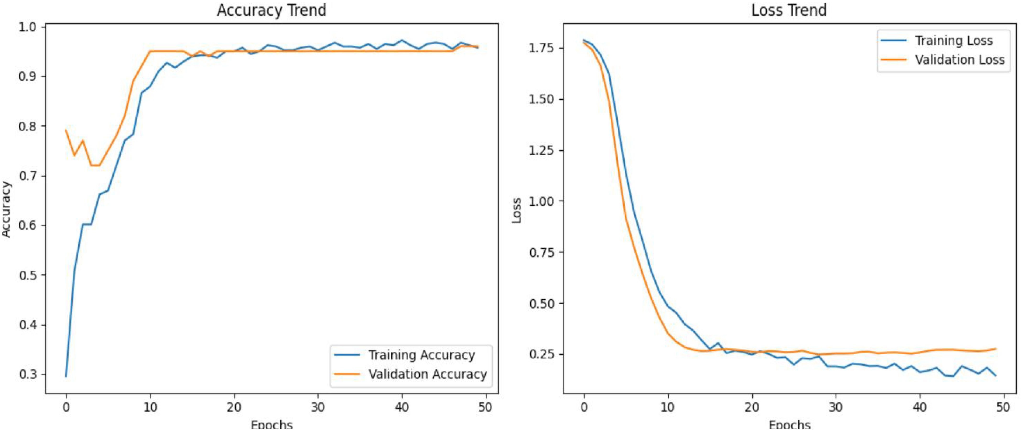
Figure 9. Accuracy, loss vs epochs curve for hybrid model (MLP WITH LSTM).

The comparison of metrics from Figure 10—Accuracy, Precision, F1-Score, and Recall—between the MLP (Multi-Layer Perceptron) and MLP with LSTM models reveals the following observations:

Figure 10

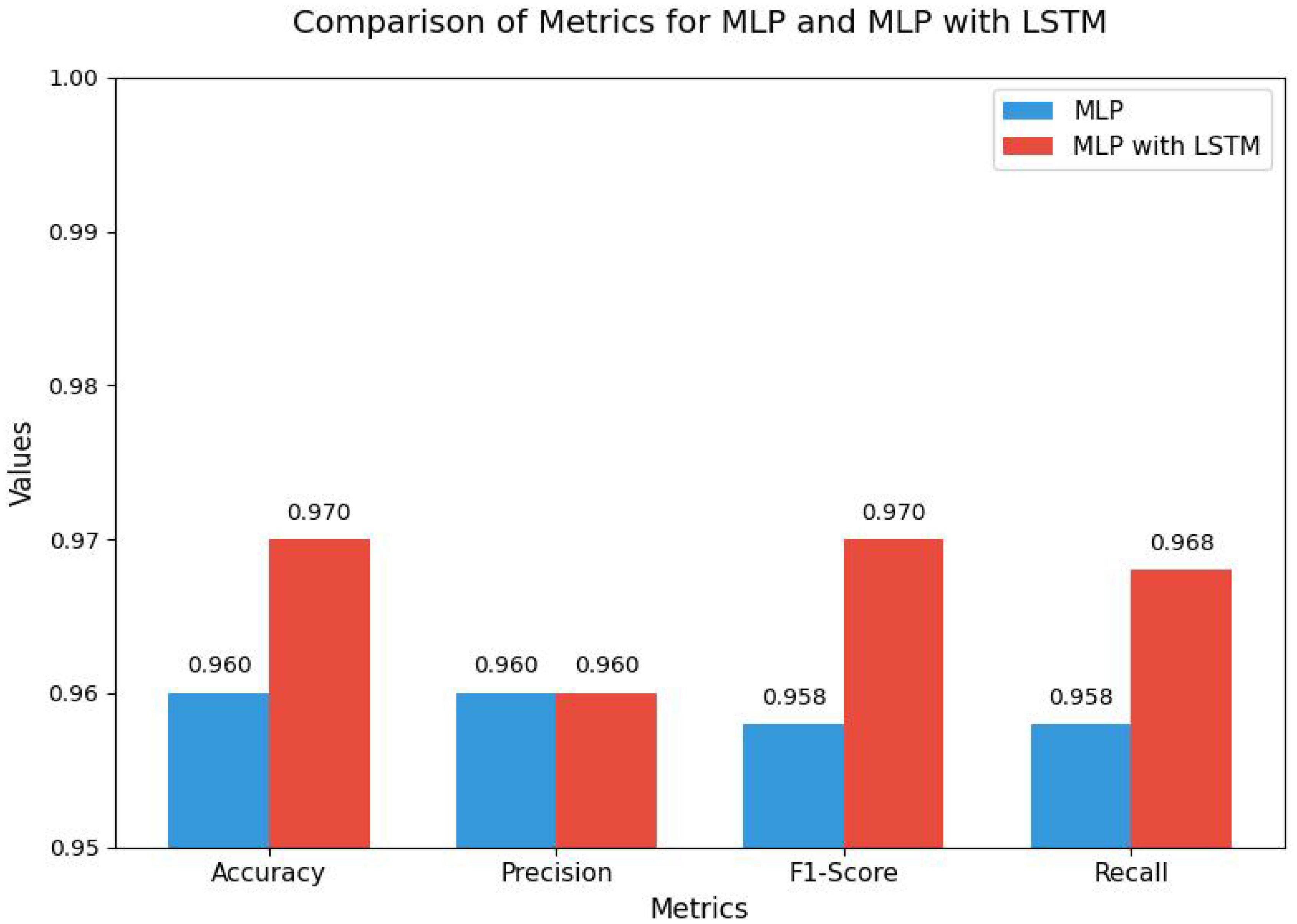
Figure 10. Comparison of MLP and MLP with LSTM.

a. Accuracy: The MLP with LSTM model achieves a higher accuracy of 0.970 compared to the MLP model’s accuracy of 0.960. This indicates that the LSTM augmentation improves the overall performance in terms of correctly classifying the data.

b. Precision: Both models achieve the same Precision value of 0.960, indicating that the models are equally effective at minimizing false positives.

c. F1-Score: The MLP with LSTM model achieves a higher F1-Score of 0.970, compared to 0.958 for the MLP model. This improvement suggests that the MLP with LSTM strikes a better balance between precision and recall.

d. Recall: The MLP with LSTM model achieves a Recall of 0.968, outperforming the MLP model, which has a recall of 0.958. This improvement implies that the MLP with LSTM is more effective at identifying all relevant instances, reducing false negatives.

The inclusion of the LSTM layer in the MLP architecture results in noticeable improvements in Accuracy, F1-Score, and Recall, while maintaining the same Precision as the standard MLP model. This highlights the superior performance of the MLP with LSTM model in tasks that require better generalization and recall capabilities, particularly for datasets where sequential dependencies play a role.

All models, including both traditional machine learning (e.g., Random Forest, XGBoost) and deep learning architectures (MLP, LSTM), were evaluated using Stratified K-Fold Cross-Validation with K = 5. This ensured that the distribution of fertility classes (Low, Medium, High) was preserved across all folds. For each model, the training and evaluation were repeated five times, and the reported performance metrics (Accuracy, Precision, Recall, F1-score) represent the average across the five folds. For deep learning models, the cross-validation process was repeated with new weight initializations for each fold to avoid data leakage and overfitting. This approach ensured robustness and generalizability of the results.

To assess the significance of model performance differences, a one-way ANOVA test was conducted on F1-scores obtained across five cross-validation folds for each model. The resulting p-value (< 0.05) indicates that the differences in F1-scores are statistically significant. Post-hoc Tukey’s HSD test revealed that XGBoost and Gradient Boosting significantly outperformed SVM and Logistic Regression.

4 SISFMA hardware testbed

A hardware prototype Artificial Intelligence based Smart Innovative Soil Fertility Monitoring Aid (AI-SISFMA) presented in Figure 11 has been made to analyze the fertility of the soil. The prototype features are as follows (a) It measures the equal distribution of fertilizer in irrigation land, (b) Fertilizer level intimation in the soil to the farmer, if it is below the required level, (c) Field officer suggestions for fertilizer level intimation via Mobile Application(d) Moisture level indicator to provide equal amount of water distribution (e) Mobile Application Development - Input from farmer, AI based Suggestion Window.

Figure 11

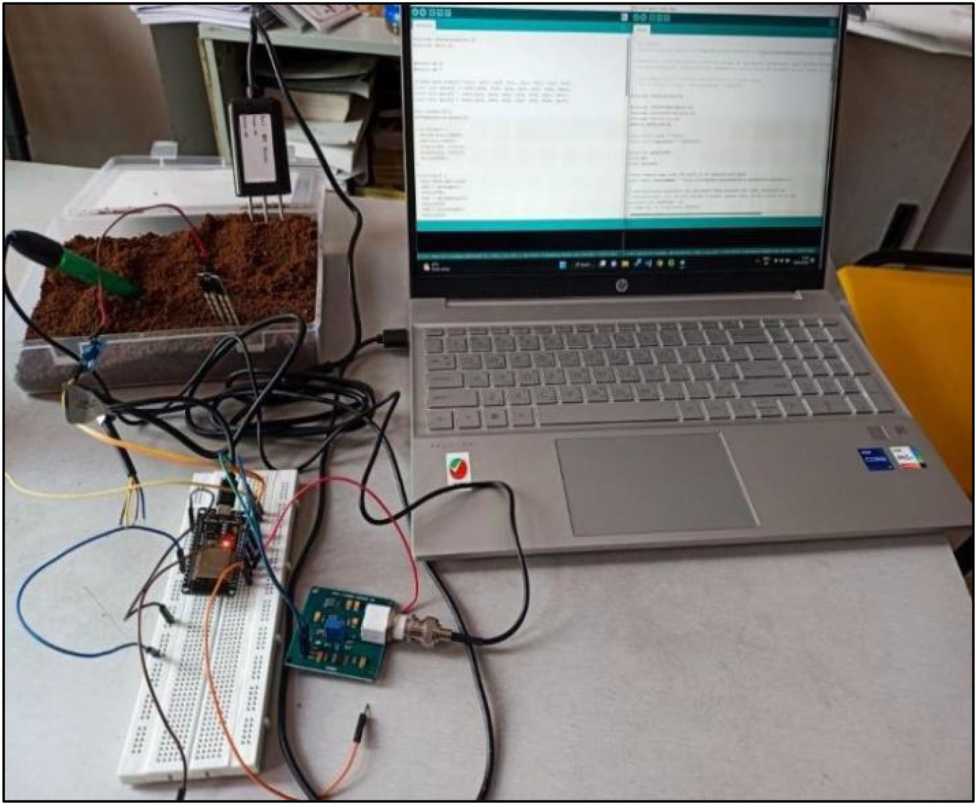
Figure 11. AI-SISFMA IoT kit.

Table 8 lists the hardware specifications of AI-SISFMA IoT kit. The prototype comprises moisture sensor (RKI-4669) for measuring the moisture level in the soil, NPK sensor for measuring nitrogen, phosphorus and potassium level in the soil, and aeration using MIJ03 sensor. Arduino microcontroller (ATmega32u4) to collect the sensed soil nutrients level, pH sensor (SKU: 235871) for measuring the pH level in the soil, Wifi module (ESP2866), GSM module (TOM-24112) and prototype android app for getting suggestions from agricultural field officer. In addition to the above sensors the farmer has the option to capture the image of his/her land to check the soil color and contamination. The NPK sensor senses the soil fertility level and if it is less than the threshold level, the farmer contacts the AFO using user friendly AI-SISFMA mobile application for suggestions regarding the amount of fertilizer to be mixed up with soil for crop farming. The data from the prototype kit and the captured image are processed by the AI based recommendation model available with the AFO. AFO verifies and suggests the best optimal solutions for the farmer in terms of fertilizer usage, moisture level and pH level to be maintained and the types of crops that can be grown on their land. This suggestion improves the better yield of a particular crop, reduces the conventional mode of soil nutrients measurement, and increases the farmer’s income.

Table 8

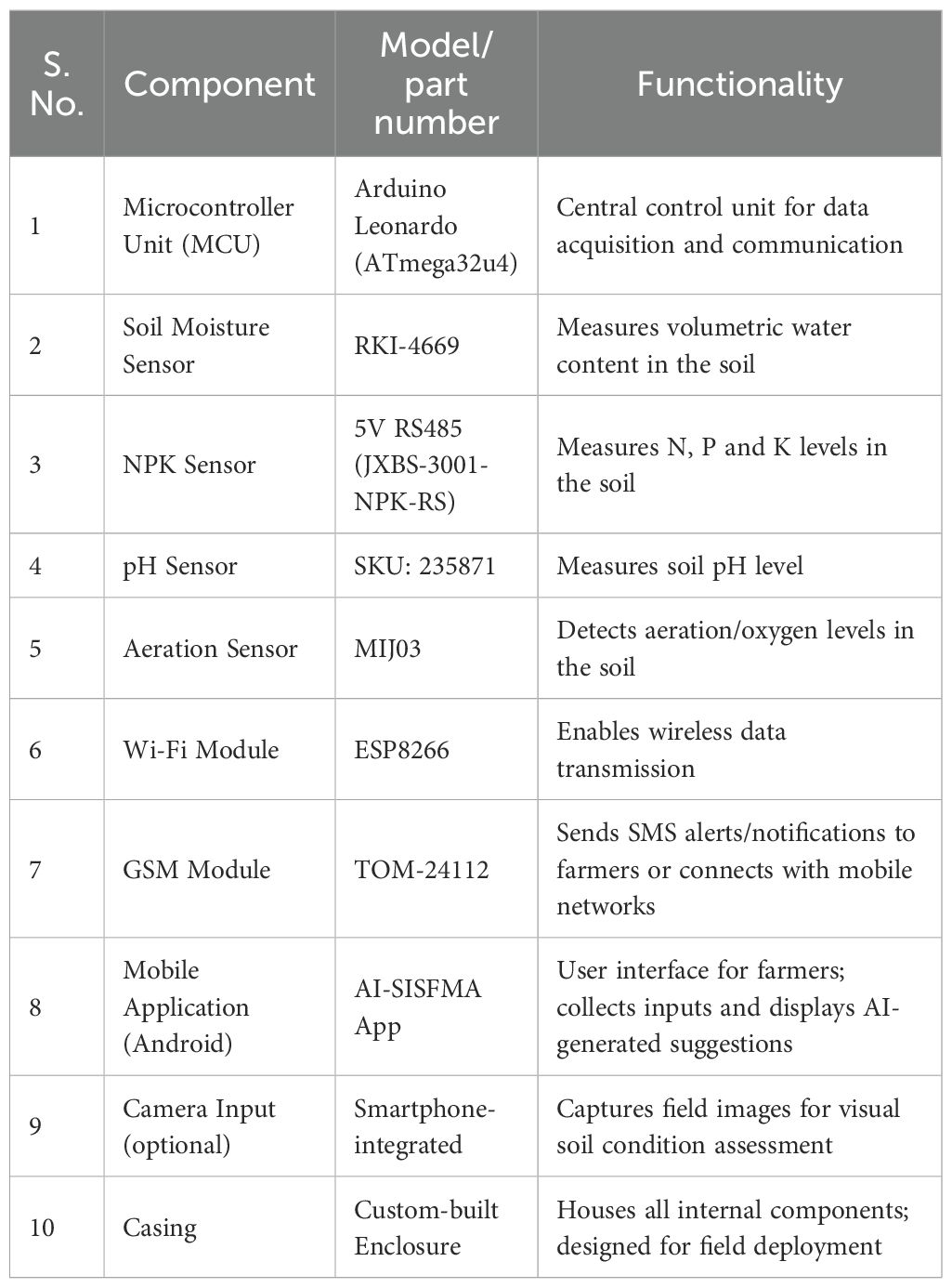
Table 8. Hardware specification of AI-SISFMA IoT kit.

The Figure 12 illustrates the casing of SISFMA kit with two views: a front view and an isometric view. The isometric view provides a 3D perspective of the casing, showing the spatial arrangement of components inside the device. This view helps to understand how different components like the MCU, power board, and pH sensor module are housed within the enclosure and how they are positioned relative to one another.

Figure 12

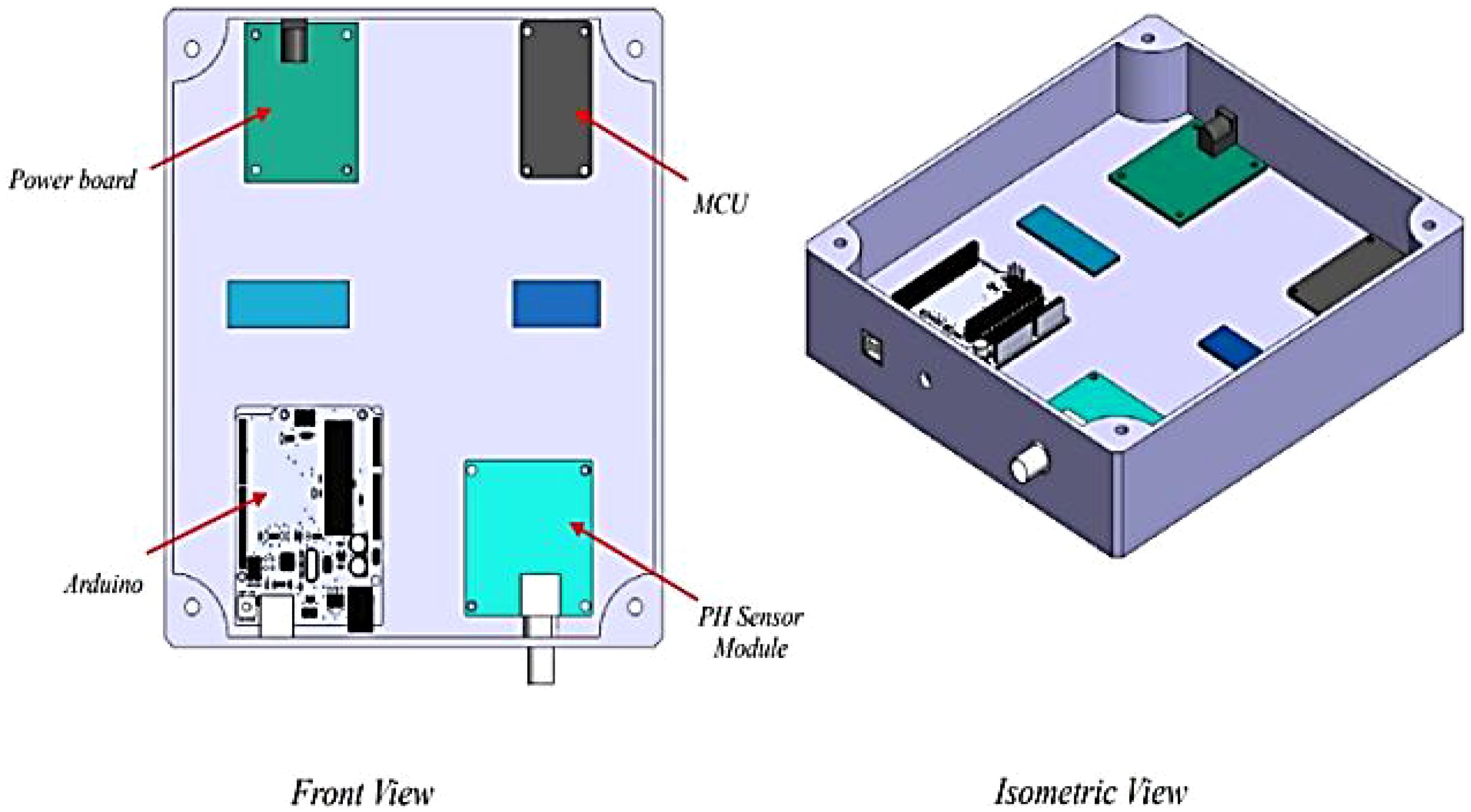
Figure 12. SISFMA kit casing.

The device is likely built to be deployed in the field, possibly in precision agriculture or soil fertility assessments, to measure soil properties directly and give farmers or researchers data that can be used for decision-making. If this device is indeed used for soil analysis, its design reflects a typical modular structure, where different sensors (like pH or moisture sensors) and processing units (MCU or Arduino) are incorporated into a robust casing for outdoor use.

Figure 13 depicts the work flow diagram of the SISFMA kit. The following are the step-by-step work involved in SISFMA.

Figure 13

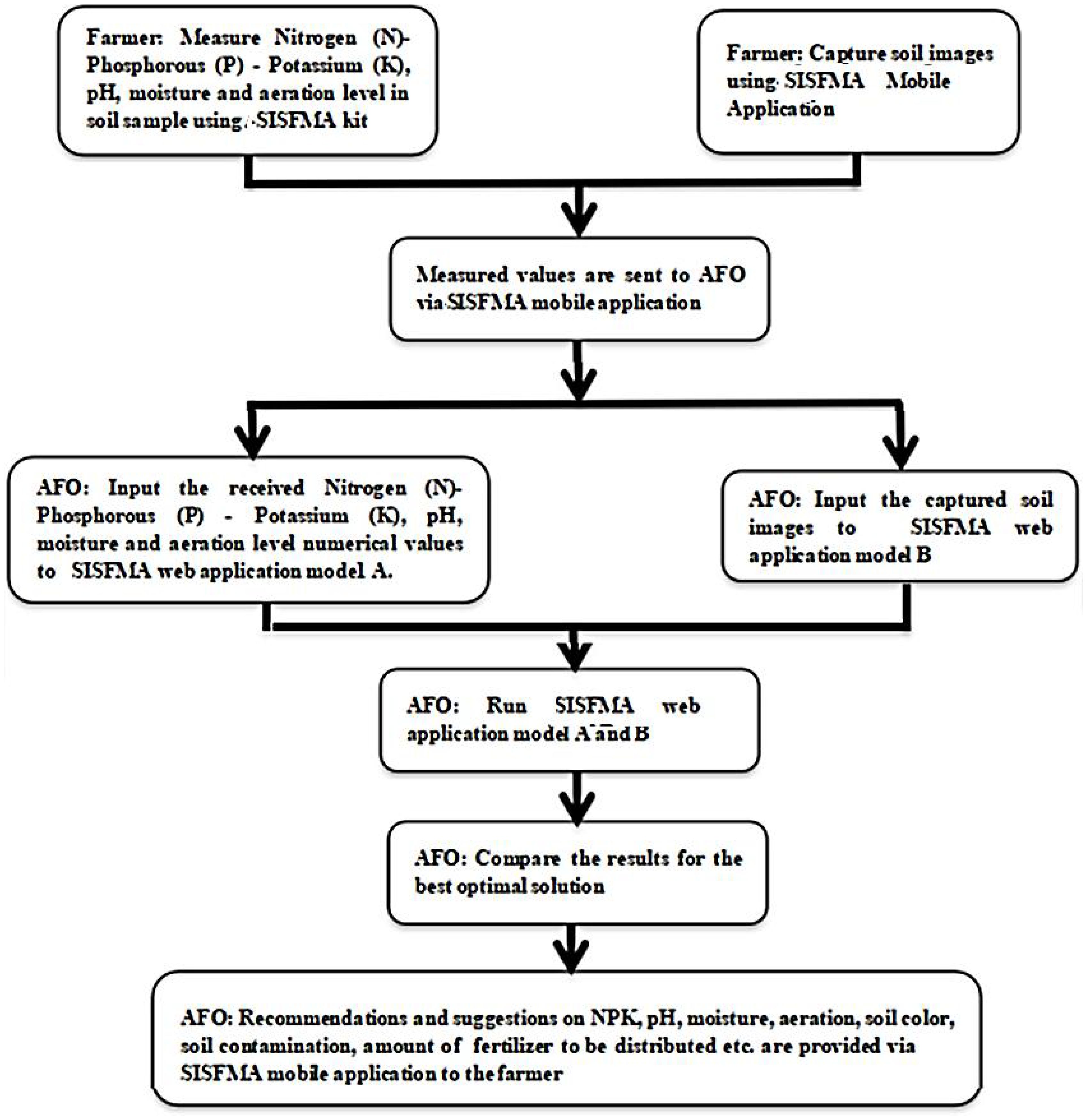
Figure 13. Workflow diagram SISFMA [Smart innovative soil fertility monitoring aid].

4.1 Data collection by farmer

The farmer uses the SISFMA kit to measure key soil properties such as N, P, K, pH, moisture, and aeration levels. These properties are essential for determining soil fertility. Along with measuring physical and chemical properties, the farmer captures soil images using the SISFMA mobile application. These images could be used for visual assessment of soil quality and structure.

4.2 Data transmission

The collected data (both measured values and images) are sent to an entity referred to as AFO (possibly Agricultural Field Officer or Agriculture Fertility Optimizer) via the SISFMA mobile application.

4.3 Data input into AI models

The AFO inputs the received measured values of nitrogen, phosphorus, potassium, pH, moisture, and aeration into SISFMA web application model A. This model likely uses numerical analysis to assess the soil fertility based on standard soil test data. The captured soil images are input into SISFMA web application model B. This model might use image processing or AI-based visual analysis (such as machine learning or computer vision) to assess additional soil characteristics, such as texture, color, or contamination.

4.4 Running AI models: run both models

The AFO runs both Model A and Model B of the SISFMA application. Each model analyzes the data based on different inputs (numerical vs. image-based analysis), and produces an assessment of the soil’s condition and fertility.

4.5 Comparison of results for optimal solution

The AFO compares the results from both models (A and B). This comparison helps in arriving at the best optimal solution, combining the numerical and visual data analysis for a comprehensive understanding of soil health.

Based on the analysis, the AFO provides recommendations and suggestions via the SISFMA mobile application. These recommendations may cover: Optimal NPK levels for fertilization; pH adjustments if the soil is too acidic or alkaline; moisture and aeration levels to ensure proper soil structure and hydration; other soil properties like soil color (which could indicate organic matter or contamination); fertilizer amounts and types to be distributed based on the fertility assessment.

This ML-based system appears to be designed for precision agriculture.

The enhancement in soil fertility management by providing tailored recommendations based on both measurable soil parameters and visual analysis is accomplished. It helps farmers optimize fertilizer use, thereby improving crop yields and promoting sustainable farming practices by reducing overuse of chemicals. The key advantages include automated Analysis, dual data approach and real time support. The SISFMA system simplifies soil analysis, making it easier for farmers to get accurate recommendations without requiring extensive technical knowledge. By combining numerical soil properties and image-based data, the system provides a more thorough analysis. The mobile and web-based platforms ensure that farmers receive quick and actionable feedback on soil management strategies.

5 Experimental results

The real time extraction of soil sample from Brahmapuram location is shown in Figure 14.

Figure 14

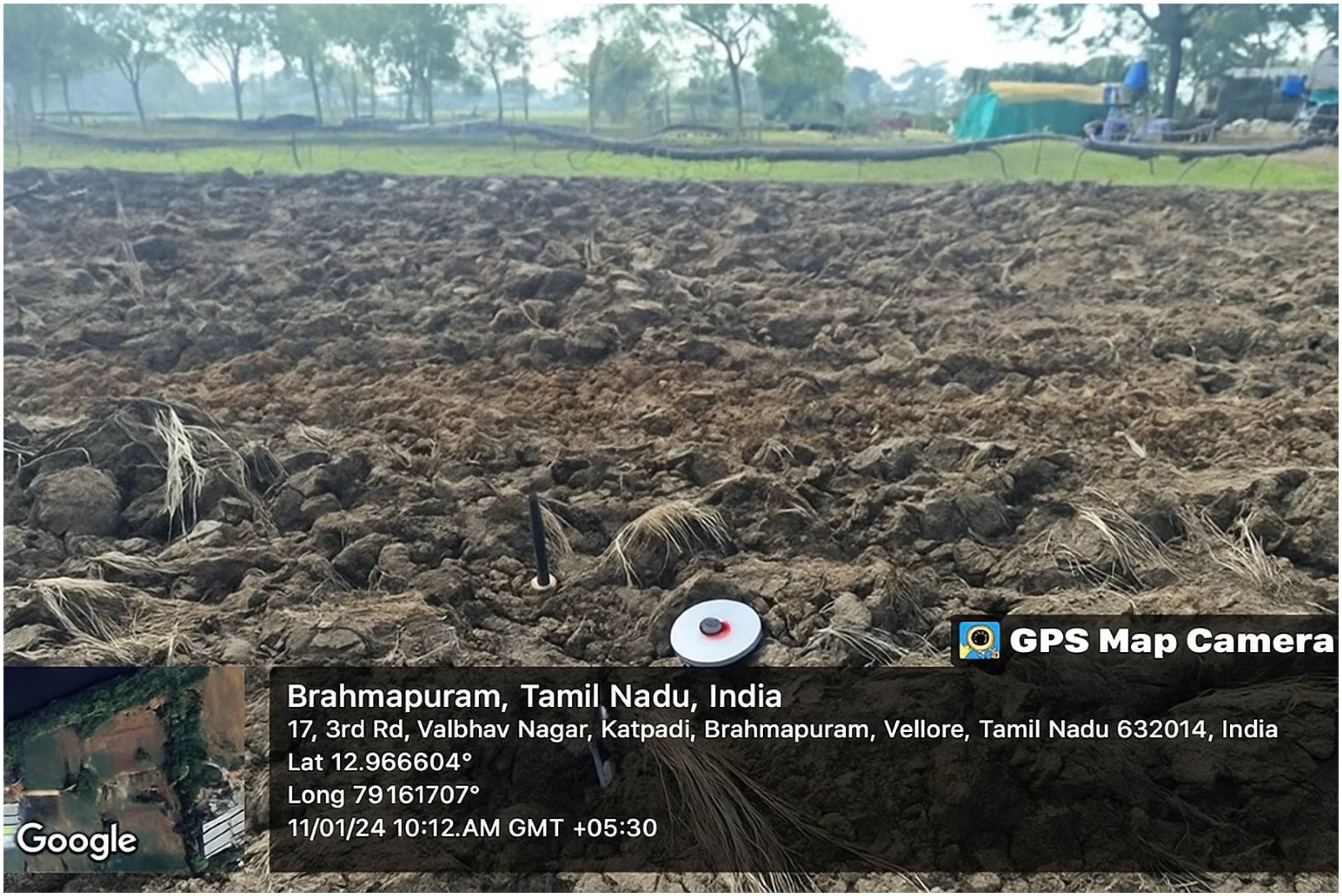
Figure 14. Real time soil extraction from Brahmapuram.

For experimental verification, the soil samples were collected from different locations in Vellore district and are presented in Table 9.

Table 9

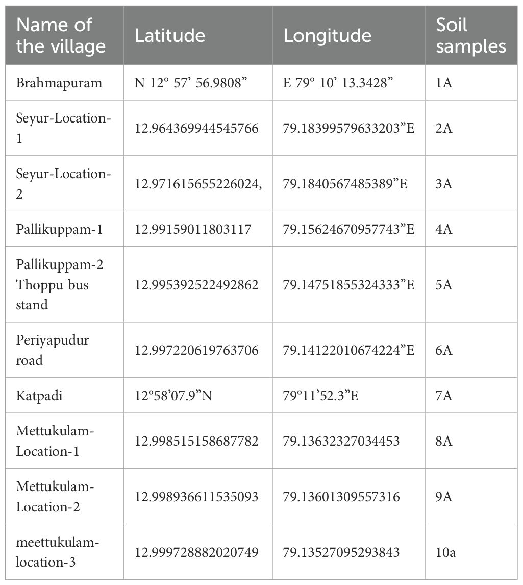
Table 9. Soil samples from different location in Vellore district.

5.1 Real time soil fertility prediction

The soil-1A (Figure 15A) has low nutrient levels, particularly nitrogen and phosphorus. It could benefit from fertilizer supplementation. Its pH is suitable for a wide variety of crops, but nutrient amendments are needed. The soil-2A (Figure 15B) is nutrient-rich and has excellent moisture retention. It should be suitable for crops requiring high nutrient levels, but drainage might need to be improved due to high moisture. The soil-3A (Figure 15C) figure is moderately fertile but lacks phosphorus. Suitable for a wide range of crops, but phosphorus amendments may be necessary to improve yield. The soil-4A (Figure 15D) is with a poor nutrient profile with very low nitrogen, phosphorus, and potassium. This soil would need significant fertilization to support plant growth. The soil-5A (Figure 15E) is with Neutral pH, but nutrient-deficient, especially in potassium. Fertilizer application is essential before planting. The soil-6A (Figure 15F) is highly acidic and nutrient-poor, requiring both pH adjustment and significant nutrient supplementation. The soil-7A (Figure 15G) is with low fertility with a slightly alkaline pH, which is suitable for certain crops like legumes then it needs nutrient enhancements for optimal growth. The soil-8A (Figure 15H) is moderately fertile but needs more phosphorus and potassium. It’s slightly acidic, which can be tolerated by most crops. The soil-9A (Figure 15I) has moderate nitrogen but lacks phosphorus and potassium. High moisture may need management depending on the crop. The soil-10A (Figure 15J) has a balanced nutrient profile with moderate amounts of nitrogen, phosphorus, and potassium.

Figure 15

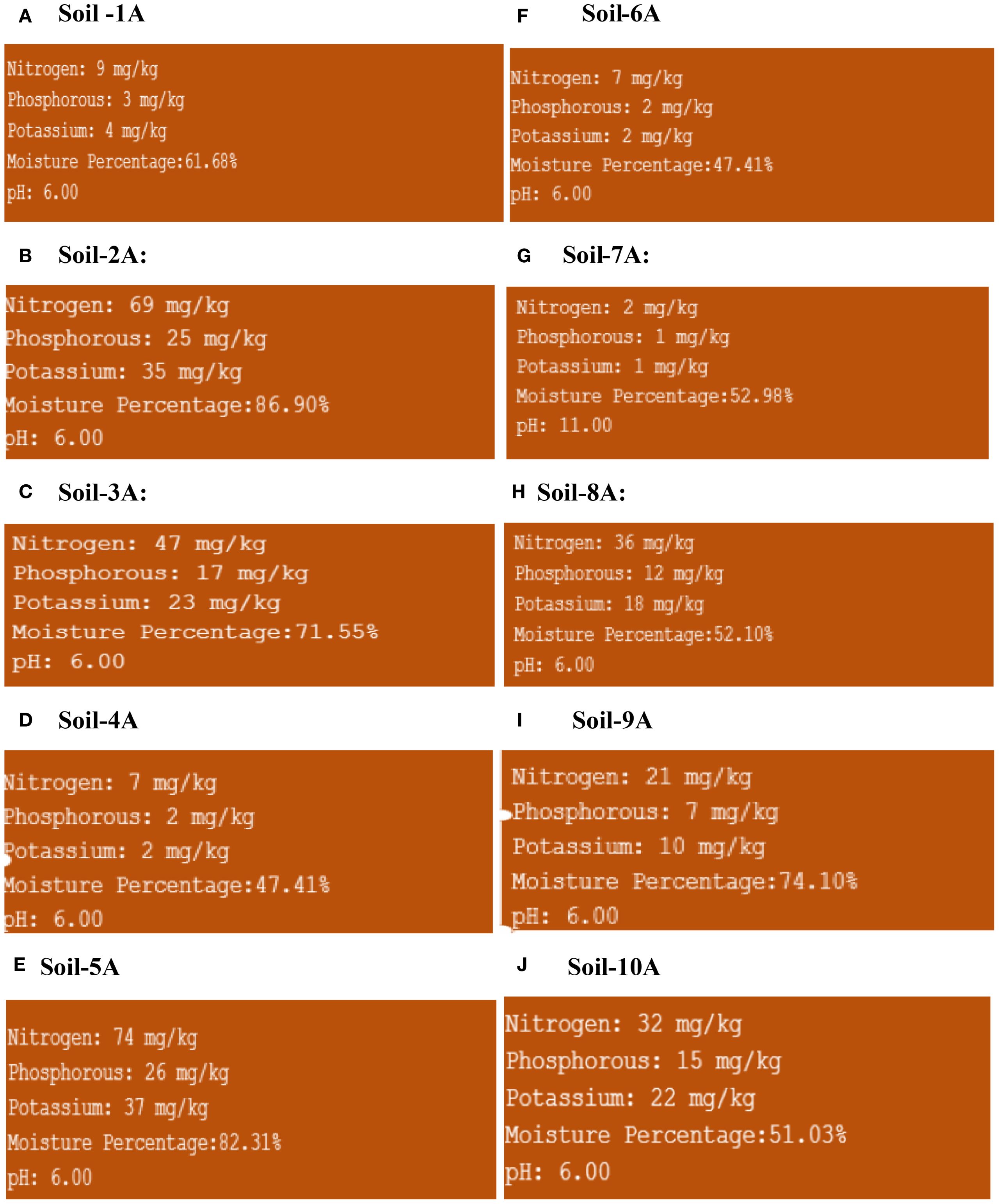
Figure 15. Soil Sample outputs (A) Soil 1A, (B) Soil 2A, (C) Soil 3A, (D) Soil 4A, (E) Soil 5A, (F) Soil 6A, (G)Soil 7A, (H)Soil 8A, (I) Soil 9A, (J) Soil 10A.

In Soil Sample - 2A (Figure 16A) the pH measured using the SISFMA kit and predicted results closely match the lab results. For Potassium, the lab results are slightly lower than both the SISFMA predictions and the kit. A similar trend is observed for Phosphorus, with the lab results being slightly lower across all methods. However, for Nitrogen, the lab results are significantly higher compared to both the SISFMA predictions and the kit.

Figure 16

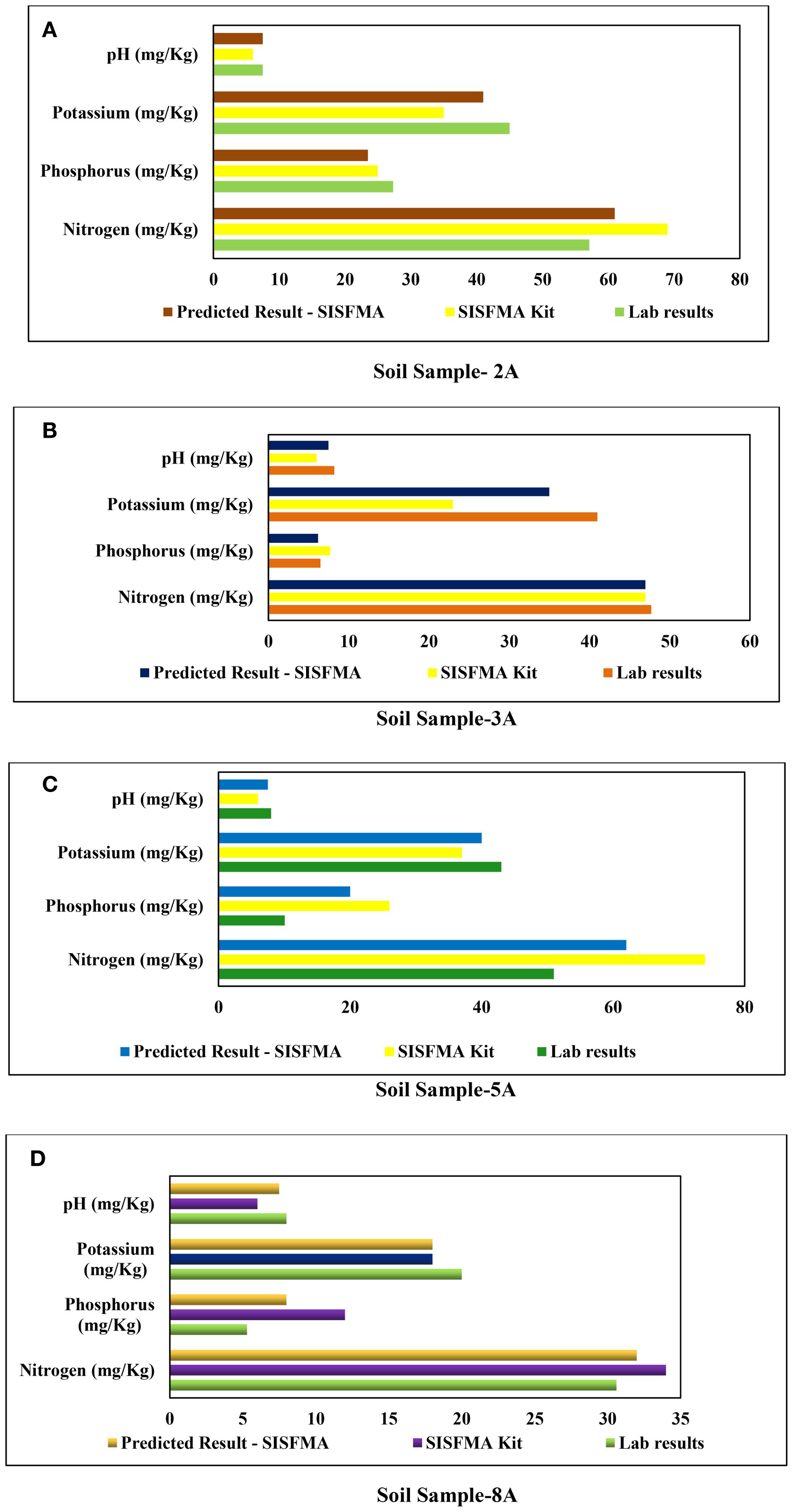
Figure 16. (A) Soil Sample- 2A. (B) Soil Sample-3A. (C) Soil Sample-5A. (D) Soil Sample-8A.

In Soil Sample - 3A (Figure 16B) the lab results for pH are higher compared to both the SISFMA predictions and the kit. In the case of Potassium, the SISFMA kit underestimates the values, while the predicted results are much closer to the lab measurements. For Phosphorus, the lab results exceed those obtained by both the SISFMA predictions and the kit. However, Nitrogen levels are consistent across all methods, showing minimal variation between the SISFMA predictions, the kit, and the lab results.

In Soil Sample - 5A (Figure 16C), the predicted results overestimate pH compared to both the lab results and the SISFMA kit, which are closely aligned. For Potassium, the SISFMA kit shows significantly higher values than both the lab results and predictions. Regarding Phosphorus, the predictions are higher than the lab results, with the SISFMA kit providing the lowest measurements. In the case of Nitrogen, the lab results indicate higher nitrogen content compared to both the predictions and the SISFMA kit.

Nitrogen values tend to be the most consistent across all methods, particularly in sample 3A. In contrast, Potassium and pH exhibit noticeable variation between methods, with the SISFMA kit often differing from the lab results. Overall, the SISFMA kit generally shows closer alignment with lab results in some cases, although the predicted values also demonstrate reliability depending on the parameter being measured.

The MAE, RMSE, and Percentage Deviation (Table 10) for key soil parameters (pH, N, P, K) across four sample sets was calculated. The maximum observed deviation is 13.26%, and the highest RMSE recorded is 3.72 mg/kg (Figure 16A Soil Sample- 3A). These results demonstrate that SISFMA’s predicted outputs are closely aligned with laboratory results, affirming the system’s reliability for field-level applications. Table 11.shows the error rates for each parameter (N, P, K, pH) measured by the kit vs lab standard.

Table 10

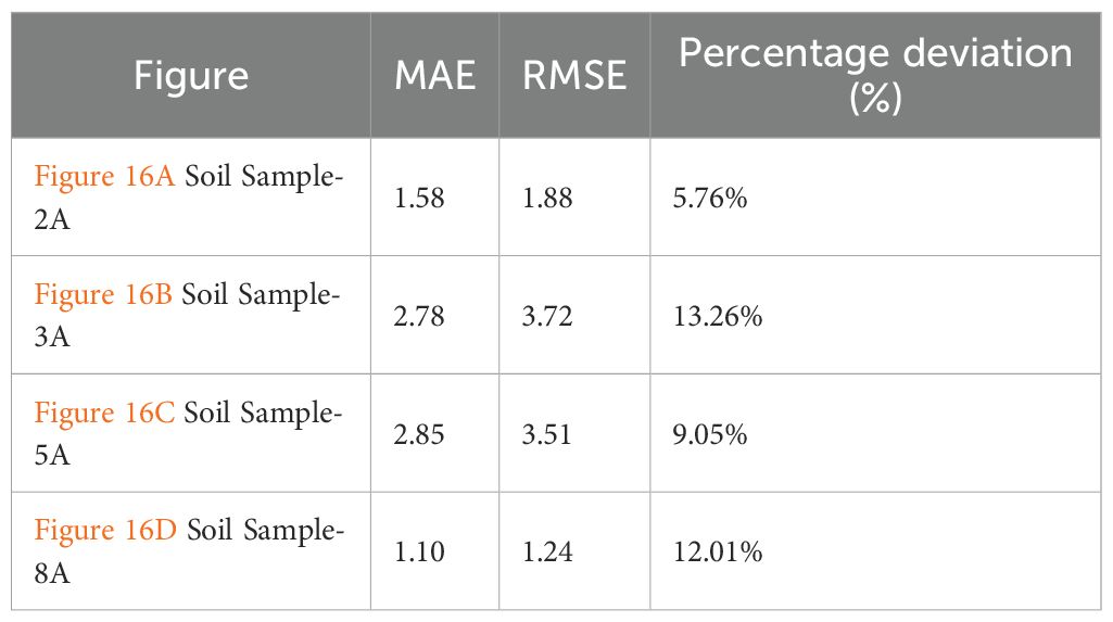
Table 10. Evaluation of SISFMA predictions against laboratory measurements for four representative soil samples (2A, 3A, 5A, 8A) shown in Figures 16A-D.

Table 11

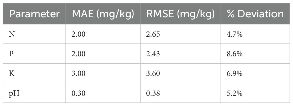
Table 11. Error rates for each parameter (N, P, K, pH) measured by the kit vs lab standard.

5.2 Feature importance and key soil indicators

The insights from feature importance analysis have been directly integrated into the SISFMA system to enhance crop advisory services. For instance, soils identified with low N and P levels were mapped to legume and pulse-based cropping recommendations, as these crops enrich nitrogen content naturally. Similarly, low pH (acidic soil) predictions triggered recommendations for lime application and pH-tolerant crops. This data-informed mapping improves both fertility correction and crop suitability, enabling sustainable practices. Notably, fields with high OC but low macronutrients were recommended compost-supplemented cereals or oilseeds. This demonstrates how predictive parameters influence both fertilizer dosing and crop decision support.

Feature importance analysis using the Gini index from the RF model (Table 12) revealed that N, P, K, and pH are the most influential features in determining soil fertility class. This aligns with standard agronomic understanding, as macronutrients and pH strongly influence crop productivity. Secondary elements like OC and EC also contributed meaningfully, while micronutrients like Zn and Fe showed lower predictive power.

Table 12

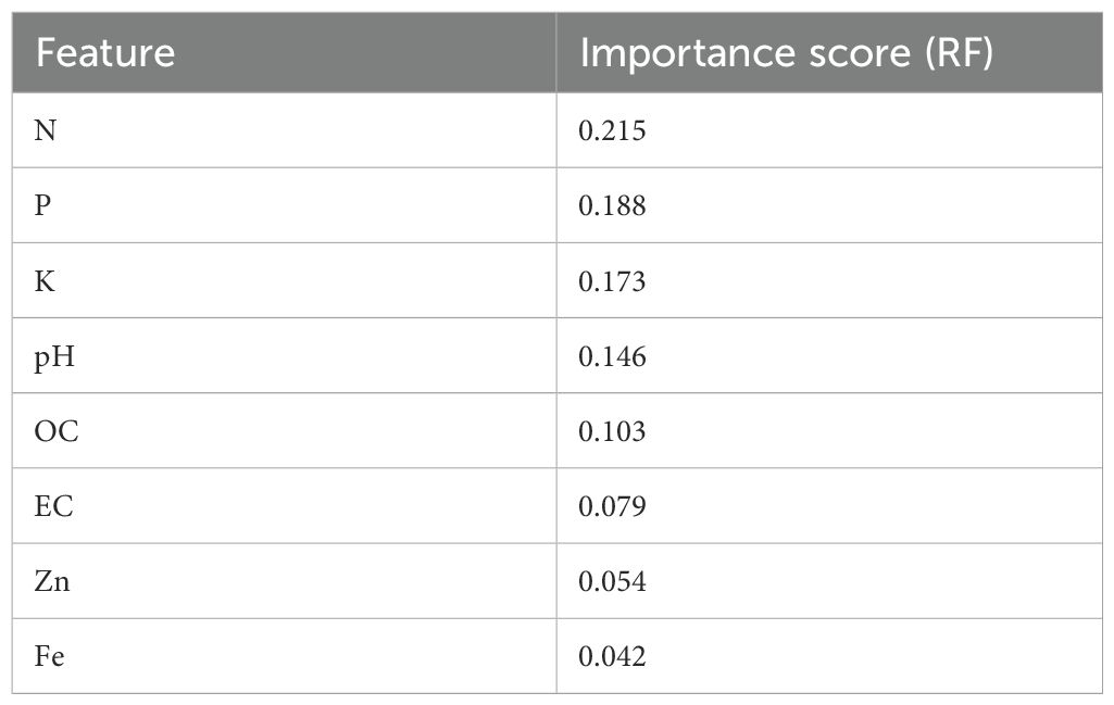
Table 12. Feature importance analysis.

6 SISFMA mobile application

The diagram (Figure 17) appears to illustrate the workflow of a mobile application named SISFMA designed for managing soil health and providing recommendations to farmers and field officers.

Figure 17

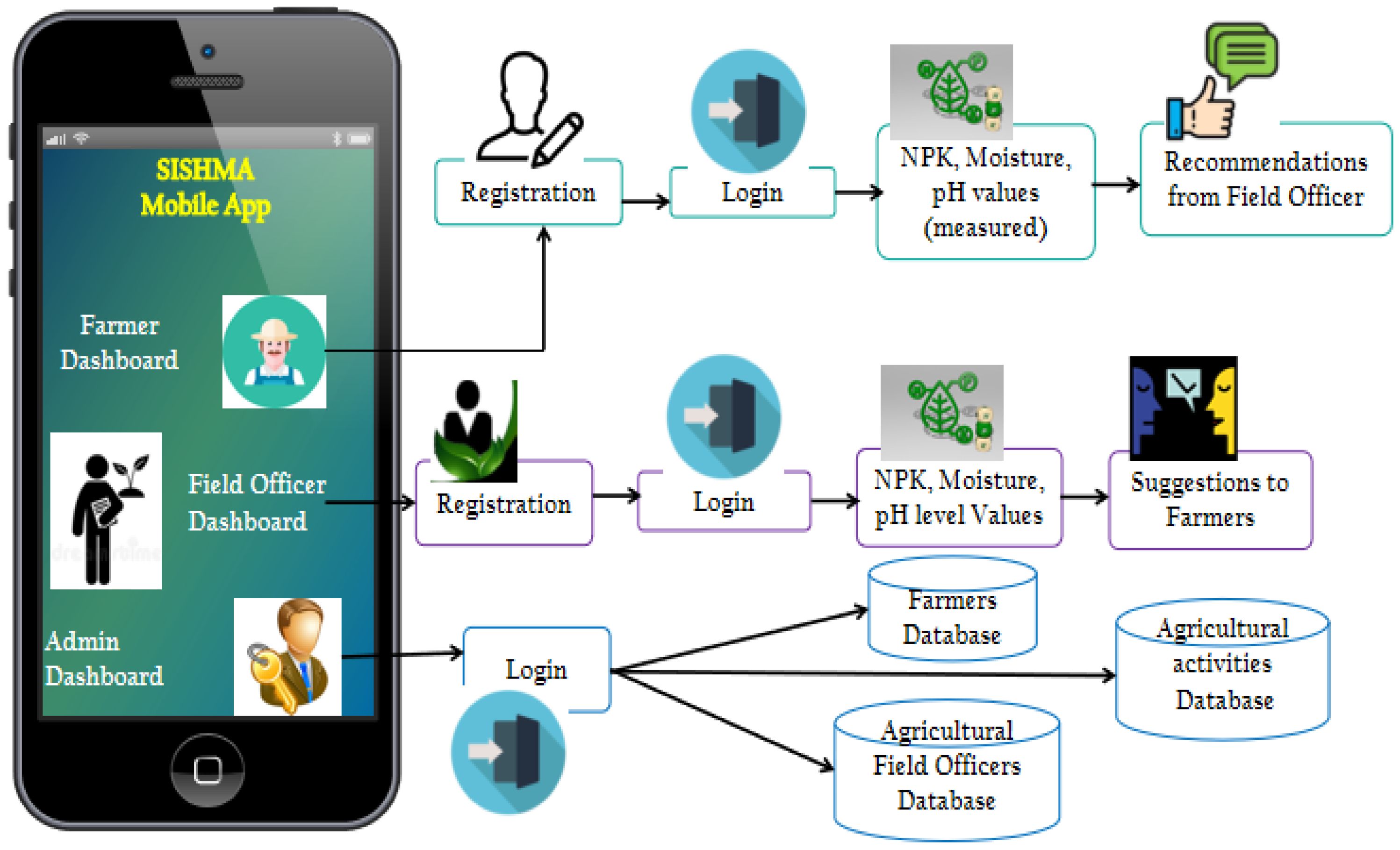
Figure 17. SISFMA multilingual mobile application dashboard.

A breakdown of the key components and interactions are given below:

1. Mobile App Interfaces consists of Farmer Dashboard, Field Officer Dashboard and Admin Dashboard. Farmer Dashboard allows farmers to interact with the system, receive suggestions, and input their soil data. Field Officer Dashboard is designed for agricultural field officers to log in and manage data, provide recommendations, and interact with farmers. Admin Dashboard manages the overall system, with access to both farmer and field officer data. Our approach aligns with the mobile-based soil monitoring systems reported previously (39), extending their functionality with real-time machine learning predictions.

2. Registration and Login Dashboard: Both farmers and field officers are required to register and then log in to access the app’s services. Once logged in, farmers and officers are linked to different workflows: Farmers provide soil data (NPK levels, moisture, pH values) that is processed and stored. Field Officers can Access the same data to make recommendations and provide advice to farmers.

3. Data Flow: After login, farmers input the measured values which are stored in a farmers’ database. The field officers access these values, analyze them, and provide tailored recommendations. Based on the soil data, farmers receive automated suggestions or advice from field officers through the app.

4. Databases: There are three databases maintained. Farmers Database that stores data related to individual farmers, including their soil measurements. Agricultural Field Officers Database that contains records of the officers interacting with the system. Agricultural Activities Database that stores information related to farming practices and recommendations provided by field officers.

5. Outputs: Based on the data collected (NPK, moisture, pH levels), field officers offer personalized recommendations to farmers. Automated or officer-provided suggestions to improve soil health and optimize agricultural practices are delivered through the app as depicted in Figure 18.

Figure 18

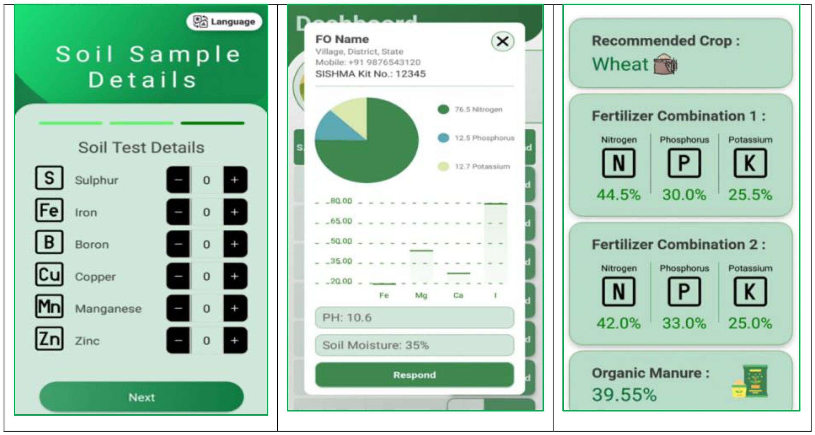
Figure 18. Screenshots of SISFMA mobile application developed.

6 Conclusion

Numerous machine learning algorithms have been employed to analyze soil fertility, that offers a sustainable and efficient alternative to traditional, labor-intensive methods. However, only a handful of these models have demonstrated notable accuracy. By integrating different sensors such as (NPK, pH and moisture), the environmental variables and meteorological data are collected and incorporating ML algorithm farmers are assisted in optimizing soil management. Initially, linear classifier models are utilized including Perceptron, Ridge Classifier, Linear Regression, SGD Classifier, and Logistic Regression. Despite achieving accuracies above 75%, these models failed to impress. The search is expanded for a superior model and explored ensemble models in the ‘scikit’ Library such as Extra trees, RF, Gradient Boosting, and Ada Boosting. Additionally, we experimented with clustering methods like Kmeans (unsupervised), and K-NN (supervised), all of which resulted in precision below 50%. Finally, Decision Trees, GaussianNB, and Support Vector Machine are also employed in the analysis. Among the models tested, the Random Forest algorithm achieved the highest accuracy (92%), highlighting its effectiveness in soil fertility prediction. Moreover, the inclusion of the LSTM layer in the MLP architecture for predicting crops results in noticeable improvements in Accuracy, F1-Score, and Recall, while maintaining the same Precision as the standard MLP model. This highlights the superior performance of the MLP with LSTM model in tasks that require better generalization and recall capabilities, particularly for datasets where sequential dependencies play a role. In summary, this work significantly advances the use of AI and ML in agriculture, making it a crucial step toward more sustainable and precise farming practices. The integration of hardware readings with machine learning models plays a crucial role in enhancing predictive accuracy and ensuring reliable decision-making. Real-time sensor data can help minimize excessive use of fertilizers, pesticides, and water, promoting environmentally friendly farming practices. Accurate predictions enable better decision-making regarding irrigation, disease prevention, and yield estimation, ultimately leading to increased productivity and profitability for farmers. By reducing chemical overuse, the system supports sustainable agriculture, preserving soil health and reducing pollution. By seamlessly combining hardware-driven insights with machine learning capabilities, the system enhances efficiency, sustainability, and economic viability, making it a valuable tool for modern precision agriculture.

Data availability statement

Publicly available datasets were analyzed in this study. This data can be found here: https://www.kaggle.com/datasets/rahuljaiswalonkaggle/soil-fertility-dataset.

Author contributions

KG: Conceptualization, Funding acquisition, Methodology, Writing – original draft, Writing – review & editing, Project administration, Supervision, Validation. KA: Conceptualization, Formal analysis, Funding acquisition, Methodology, Writing – original draft, Writing – review & editing. PS: Writing – review & editing, Data curation, Software.

Funding

The author(s) declare financial support was received for the research and/or publication of this article. SISHMA [Smart Innovative Soil Health Monitoring Aid] is funded by Department of Science and Technology [DST] under Device Development Program [DDP]. The funding amount was $5,231 during the period 2021- 2023.

Acknowledgments

The authors would like to Vellore Institute of Technology, Chennai for providing the infrastructure facilities; DST for providing the funding and National Agro Foundations, Chennai for providing the soil test reports for the samples provided.

Conflict of interest

The authors declare that the research was conducted in the absence of any commercial or financial relationships that could be construed as a potential conflict of interest.

Generative AI statement

The author(s) declare that no Generative AI was used in the creation of this manuscript.

Any alternative text (alt text) provided alongside figures in this article has been generated by Frontiers with the support of artificial intelligence and reasonable efforts have been made to ensure accuracy, including review by the authors wherever possible. If you identify any issues, please contact us.

Publisher’s note

All claims expressed in this article are solely those of the authors and do not necessarily represent those of their affiliated organizations, or those of the publisher, the editors and the reviewers. Any product that may be evaluated in this article, or claim that may be made by its manufacturer, is not guaranteed or endorsed by the publisher.

References

1. Ahmadi K, Meyer C, and Ruehlmann J. Rapid in-field soil analysis of plant-available nutrients and pH for precision agriculture—a review. Precis Agriculture. (2021) 23:45–65. doi: 10.1007/s11119-021-09806-9

Crossref Full Text | Google Scholar

2. Tessema M, Tilahun S, and Demissie A. Use of soil spectral reflectance to estimate texture and fertility affected by land management practices in Ethiopian tropical highland. PloS One. (2022) 17:e0270629. doi: 10.1371/journal.pone.0270629

PubMed Abstract | Crossref Full Text | Google Scholar

3. Mulla DJ. How can soil quality be accurately and quickly studied? A review Agronomy. (2013) 13:786–802. doi: 10.3390/agronomy14081682

Crossref Full Text | Google Scholar

4. Lv H, Jia H, and Zhao G. Effects of balancing exchangeable cations Ca, Mg, and K on the growth of tomato seedlings (Solanum lycopersicum L.) based on increased soil cation exchange capacity. Agronomy. (2024) 14:629. doi: 10.3390/agronomy14030629

Crossref Full Text | Google Scholar

5. Guo R, Shi L, and Yang Y. Germination, growth, osmotic adjustment and ionic balance of wheat in response to saline and temperature stresses. J Crop Sci Biotechnol. (2023) 55:667–79. doi: 10.1007/s12356-023-1234

Crossref Full Text | Google Scholar

6. Hatamzadeh A, Nalousi MA, Ghasemnezhad M, and Biglouei MH. Soil erosion and its impacts on plant health in agricultural systems. BMC Plant Biol. (2023) 70:538–48. doi: 10.1186/s12870-023-12345

Crossref Full Text | Google Scholar

7. Blanco-Sepúlveda R, Enríquez-Narváez F, and Lima F. Effectiveness of conservation agriculture (tillage vs. vegetal soil cover) to reduce water erosion in maize cultivation (Zea mays L.): An experimental study in the sub-humid uplands of Guatemala. Geoderma. (2021) 404:115336. doi: 10.1016/j.geoderma.2021.115336

Crossref Full Text | Google Scholar

8. Deng C, Zhang G, Liu Y, Nie X, Li Z, Liu J, et al. Advantages and disadvantages of terracing: A comprehensive review. Int Soil Water Conserv Res. (2021) 9:344–59. doi: 10.1016/j.iswcr.2021.03.003

Crossref Full Text | Google Scholar

9. Li C, Chen G, Zeng G, and Ye J. The study of soil fertility spatial variation feature based on GIS and data mining. In: Computer and Computing Technologies in Agriculture VI, vol. 393. Springer Berlin Heidelberg, Heidelberg (2013). p. 211–20.

Google Scholar

10. Rajeswari V and Arunesh K. Analysing soil data using data mining classification techniques. Indian J Sci Technol. (2016) 9:1–4. doi: 10.17485/ijst/2016/v9i19/93873

Crossref Full Text | Google Scholar

11. Xu C, Xu X, Liu M, Yang J, Zhang Y, and Li Z. Developing pedotransfer functions to estimate the Sindex for indicating soil quality. Ecol Indic. (2017) 83:338–45. doi: 10.1016/j.ecolind.2017.08.011

Crossref Full Text | Google Scholar

12. Kouadio L, Deo R, Mittahalli Byrareddy V, Adamowski J, Mushtaq S, and Nguyen V. Artificial intelligence approach for the prediction of Robusta coffee yield using soil fertility properties. Comput Electron Agric. (2018) 155:324–38. doi: 10.1016/j.compag.2018.10.014

Crossref Full Text | Google Scholar

13. John K, Abraham Isong I, Michael Kebonye N, Okon Ayito E, Chapman Agyeman P, and Marcus Afu S. Using machine learning algorithms to estimate soil organic carbon variability with environmental variables and soil nutrient indicators in an alluvial soil. Land (Basel). (2020) 9:487. doi: 10.3390/land9120487

Crossref Full Text | Google Scholar

14. Rajamanickam J and Savitha SDM. Predictive model construction for prediction of soil fertility using decision tree machine learning algorithm. INFOCOMP J Comput Sci. (2021) 20:49–55. doi: 10.26524/krj.2021.5

Crossref Full Text | Google Scholar

15. Pant J, Pant P, Pant RP, Bhatt A, Pant D, and Juyal A. Soil quality prediction for determining soil fertility in Bhimtal block of Uttarakhand (India) using machine learning. Int J Anal Appl. (2021) 19:91–109. doi: 10.28924/2291-8639-19-2021-91

Crossref Full Text | Google Scholar

16. Al Masmoudi Y, Bouslihim Y, Doumali K, Hssaini L, and Ibno Namr K. Use of machine learning in Moroccan soil fertility prediction as an alternative to laborious analyses. Model Earth Syst Environ. (2022) 8:3707–17. doi: 10.1007/s40808-021-01329-8

Crossref Full Text | Google Scholar

17. Varshitha DN and Choudhary S. Soil fertility and yield prediction of coffee plantation using machine learning technique. Res J Agric Sci. (2022) 3:514–8.

Google Scholar

18. Sharma P, Singh M, and Kumar A. Application of machine learning models for soil fertility classification using spectral data. Agric Inf. (2022) 14:112–20.

Google Scholar

19. Bhattacharya S, Bera A, and Bhattacharya K. Soil fertility classification using support vector machines and remote sensing data. J Soil Sci Environ Manag. (2021) 12:92–101.

Google Scholar

20. Bhandari R, Sharma P, Singla S, and Kang S. Predictive analysis of soil fertility using supervised machine learning techniques for enhanced agricultural productivity. Int J System Assur Eng Manage. (2025). doi: 10.1007/s13198-025-02919-w

Crossref Full Text | Google Scholar

21. Vhatkar KN, Koparde SA, Kothari S, Sarwade J, and Sakur K. Enhancing prediction of crop yield and soil health assessment for sustainable agriculture using machine learning approach. MethodsX. (2025) 14:103418. doi: 10.1016/j.mex.2025.103418

PubMed Abstract | Crossref Full Text | Google Scholar

22. Jaiswal R. Soil fertility dataset. Available online at: https://www.kaggle.com/datasets/rahuljaiswalonkaggle/soil-fertility-dataset (Accessed October 10, 2024).

Google Scholar

23. Gupta N, Sharma S, and Verma P. Application of logistic regression for predicting soil fertility based on soil physicochemical properties. J Environ Manag. (2020) 245:142–50.

Google Scholar

24. Mebrate A, Zeray N, Kippie T, and Haile G. Determinants of soil fertility management practices in Gedeo Zone, Southern Ethiopia: logistic regression approach. Heliyon. (2022) 8:e08820. doi: 10.1016/j.heliyon.2022

PubMed Abstract | Crossref Full Text | Google Scholar

25. Patel J, Singh R, and Tripathi P. Soil fertility prediction using K-nearest neighbors algorithm in precision agriculture. J Agric Inf. (2019) 10:45–55.

Google Scholar

26. Rajamanickam J and Savitha M. Mining agricultural data to predict soil fertility using ensemble boosting algorithm. Int J Inf Commun Technol Hum Dev. (2022) 14:1–10. doi: 10.4018/IJICTHD.299414

Crossref Full Text | Google Scholar

27. Kumar S and Goyal P. Predicting soil fertility using gradient boosting machines: A case study in precision agriculture. Comput Electron Agric. (2021) 185:106165. doi: 10.1016/j.compag.2021.106165

Crossref Full Text | Google Scholar

28. Longchamps L, Mandal D, and Khosla R. Assessment of soil fertility using induced fluorescence and machine learning. Sensors. (2022) 22:4644. doi: 10.3390/s22124644

PubMed Abstract | Crossref Full Text | Google Scholar

29. Ramar B and Narashiman K. A novel ensemble fuzzy neural network classifier simulator algorithm for anomaly detection from soil nutrient sample experiments. Period Mineral. (2022) 91:94–119.

Google Scholar

30. Fathololoumi S, Vaezi AR, Alavipanah SK, Ghorbani A, Saurette D, and Biswas A. Improved digital soil mapping with multitemporal remotely sensed satellite data fusion: A case study in Iran. Sci Total Environ. (2020) 721:137703. doi: 10.1016/j.scitotenv.2020.137703

PubMed Abstract | Crossref Full Text | Google Scholar

31. Devidhanshrii S, Dhivya S, and Shanmugavadivu R. Multiobjective convolution neural network towards soil nutrients classification for crop recommendation based on spectral and spatial properties using Landsat hyperspectral images. J Pharm Negat Results. (2022) 13:2021–31. doi: 10.47750/pnr.2022.13.S09.244

Crossref Full Text | Google Scholar

32. Chatterjee R and Lal R. Application of K-means clustering for soil fertility assessment and precision farming. Soil Sci J. (2022) 9:88–105. doi: 10.1016/j.soilsci.2022.01.005

Crossref Full Text | Google Scholar

33. Patil P, Kuligod V, Gundlur S, Katti J, Nagaral I, Shikrashetti P, et al. Soil fertility mapping in Dindur sub-watershed of Karnataka for site specific recommendations. J Indian Soc Soil Sci. (2016) 64:381–90. doi: 10.5958/0974-0228.2016.00050.5

Crossref Full Text | Google Scholar

34. Jia X, Fang Y, Hu B, Yu B, and Zhou Y. Development of soil fertility index using machine learning and visible-near-infrared spectroscopy. Land. (2023) 12:2155. doi: 10.3390/land12122155

Crossref Full Text | Google Scholar

35. Folorunso O, Ojo O, Busari M, Adebayo M, Joshua A, Folorunso D, et al. Exploring machine learning models for soil nutrient properties prediction: A systematic review. Big Data Cogn Comput. (2023) 7:113. doi: 10.3390/bdcc7020113

Crossref Full Text | Google Scholar

36. Sujatha M and Jaidhar CD. Machine learning-based approaches to enhance the soil fertility—A review. Expert Syst Appl. (2024) 240:122557. doi: 10.1016/j.eswa.2023.122557

Crossref Full Text | Google Scholar

37. Raut J and Mittal S. Soil fertility and crop recommendation using machine learning and deep learning techniques: A review. Turk J Comput Math Educ. (2020) 11:1119–27. doi: 10.17762/turcomat.v11i2.12855

Crossref Full Text | Google Scholar

38. Van Houdt G, Mosquera C, and Nápoles G. A review on the long short-term memory model. Artif Intell Rev. (2020) 53:5929–55. doi: 10.1007/s10462-020-09838-1

Crossref Full Text | Google Scholar

39. Gulhane VA, Rode SV, and Pande CB. Correlation analysis of soil nutrients and prediction model through ISO cluster unsupervised classification with multispectral data. Multimed Tools Appl. (2023) 82:2165–84. doi: 10.1007/s11042-022-13276-2

Crossref Full Text | Google Scholar