Mapping soil salinity using machine learning and remote sensing data in semi-arid croplands

Soil salinity significantly constrains agricultural productivity and land sustainability, particularly in irrigated areas. While, remote sensing offers large-scale monitoring capacity, but its accuracy depends on how effectively spectral information is integrated with advanced modeling approaches. This study evaluates the performance of a combined approach based on machine learning (ML) algorithms and satellite-derived predictors for soil salinity mapping in the Béni Amir Sub-perimeter of Tadla plain, Morocco. A total of 43 topsoil samples (0–10 cm) were collected and analyzed for electrical conductivity (ECe) and resampled to 144 samples for model training and testing. Predictor Variables were derived from Landsat-8 OLI data, including salinity indices (OLI-SI, SI, SI1), intensity indices (Int1, Int2), brightness index (BI), land degradation index (LDI), and reflectance values of selected spectral bands (B2-B7) were standardized and transformed with PCA to address multicollinearity. Four ML algorithms, Random Forest (RF), K-Nearest Neighbors (KNN), Support Vector Regressor (SVR), and Multi-Layer Perceptron (MLP) were tested. The results show that the Ece ranges from 0.84 to 10.28 dS/m with a standard deviation of 2.29 dS/m, indicating substantial salinity variability across the Béni Amir sub-perimeter. Individual predictors exhibited moderate correlation with Ece (R = 0.34-0.72). Among the applied models, KNN achieved the highest accuracy (mean coefficient of determination (R²) = 0.75 [0.73-0.77]; Root Mean Square Error (RMSE) = 0.61 dS/m). The resulting maps revealed a consistent southwestward increase in salinity, following the regional hydraulic flow. KNN classified 49% of the area as moderately saline, 22% as slightly saline, and 20% as non-saline, while the strongly and extremely saline classes covered 8.4% and 0.6%, respectively. RF, SVR, and MLP showed comparable trends, with moderately saline areas ranging between 30-41% and strongly to extremely saline soils below 10%. These findings demonstrated that combining satellite-derived data with ML enables a reliable assessment of soil salinity, supporting management of irrigated agroecosystems.

1 Introduction

In the era of climate change, salinization heavily affects soil quality, especially in arid environments where water resources are limited (1, 2). Soil salinization poses an increasing threat to sustainable agriculture, particularly in arid and semi-arid regions where irrigation is crucial for maintaining crop yields (3). Salinity reduces soil fertility, impairs plant growth, and leads to significant yield losses, posing challenges to global food security. According to the FAO, salt-affected soils cover 424 million hectares of topsoil (0–30 cm) and 833 million hectares of subsoil (30–100 cm), based on 73% of the land mapped so far (4). Overall, soil salinization affects approximately 1 billion hectares of land, including over 20% of irrigated croplands (5, 6).

In Morocco, about 16% of the croplands are affected by salinity, resulting in a significant reduction in agricultural productivity and posing a threat to land sustainability (7). The Tadla Plain, one of the country’s main irrigated areas, is particularly vulnerable. Multiple factors, including recurrent drought, groundwater overexploitation, inefficient irrigation practices, and the use of saline water, contribute to the accumulation of salinity (8). In addition, inadequate drainage infrastructure accelerates secondary salinization (9). Previous studies in the Tadla plain (10, 11), have highlighted the role of land use in controlling salinity patterns, emphasizing the need for accurate spatial assessments to support management strategies.

Traditional methods for soil salinity assessment rely on field sampling, laboratory electrical conductivity (EC) analysis, and GIS-based interpolation (12). Nevertheless, these provide reliable point-based measurements; they are costly, labor-intensive, and limited in spatial and temporal coverage. Remote sensing techniques offer an efficient alternative for large-scale monitoring (13). Landsat-8 OLI provides free, continuous medium-resolution imagery with a long archive and spectral bands that capture soil characteristics influenced by salinity, making it a reliable source for monitoring soil salinity patterns. Numerous studies (14–16) have demonstrated the effectiveness of Landsat-8 OLI for deriving salinity indices and mapping salt-affected soils across different agroecological regions.

Recent advances in machine learning (ML) algorithms have proven their ability to analyze complex interactions between remote sensing variables and soil properties (17–19). Algorithms such as Random Forest (RF), Artificial Neural Networks (ANN), and Support Vector Regression (SVR) have been applied in various agroecological areas, demonstrating accuracy in mapping soil salinity. Wang et al. (20). compared the performance of Landsat-8 OLI and Sentinel-2 MSI in soil salinity detection using Multivariable Linear Regression (MLR). Similarly, Aksoy et al. (15) compared the efficiency of eXtreme Gradient Boosting (XGBoost) and RF algorithms in estimating soil salinity using Landsat-8 OLI based indices, environmental covariates, and EC values. Fu et al. (21) developed and compared soil salinity indices using RF, Support Vector Machine (SVM), and XGBoost models. Naimi et al. (22) modeled soil salinity using spectral indices derived from Sentinel-2 and environmental variables, evaluating K-nearest neighbors (KNN) alongside RF, SVM, and ANN. More recently, Thangarasu et al. (23) applied RF, ANN, and SVM using various satellite-derived from Landsat 8/9 data as variables to map soil salinity. However, in Morocco, and particularly in the Tadla plain, ML-based salinity mapping remains limited, despite the growing need for accurate and cost-effective monitoring tools.

This study investigates the integration of ML algorithms and Landsat-8 OLI data to assess soil salinity in the Béni Amir sub-perimeter of the Tadla plain. This paper aims to compare the performance of four ML models (RF, SVR, ANN, and KNN) for salinity mapping and prediction with limited data, and to generate salinity maps to support sustainable management of irrigated areas.

2 Materials and methods

2.1 Study area and background

The current work was conducted in the Béni Amir irrigated sub-perimeter of the Tadla Plain, covering 674 km² in central Morocco (Figure 1). The Tadla Plain is a major hydro-agricultural region of Central Morocco. Formerly barren and exploited for pastoral purposes, this region has become a fertile agricultural area following the installation of an irrigation network, and nowadays contributing to a large proportion of national agricultural production, up to 30% for sugar beets, 12% for fodder, 11% for citrus fruits and olives, 10% for market gardening, 6% for cereals and 10% for milk (11). Since the development and commissioning of the irrigated perimeter, the salt-affected area of agricultural lands has been steadily increasing (10). Irrigation water sources include both shallow groundwater and surface water from the Oum Er Rbia River. Reported salinities are on the order of about 3.2 g/L for groundwater and about 1.3 g/L for the Oum Er Rbia surface water (8). In practice, some farmers also blend surface water with groundwater at the field or parcel scale (24), which can further vary the salinity of applied irrigation water across the perimeter. The irrigation network in the region, managed by the Regional Office for Agricultural Development of Tadla (ORMVAT) and supplied by the Oum Er Rbia River, primarily relies on surface (gravity) irrigation, which leads to considerable water losses due to inefficient infrastructure and evaporation. Although some farmers use sprinkler systems, a growing number are shifting toward drip irrigation to improve water-use efficiency (25).

Figure 1

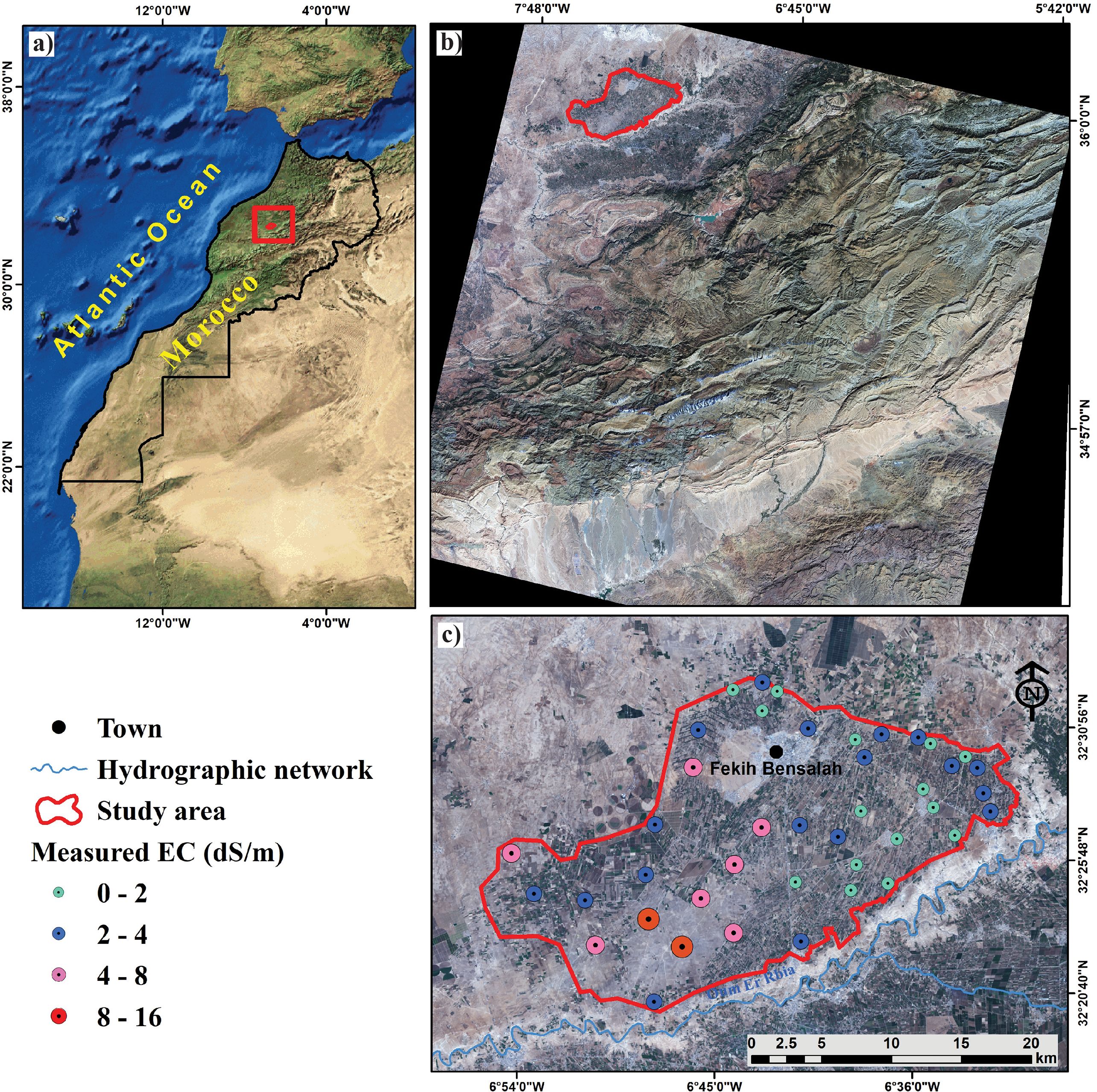
Figure 1. Location of the Tadla Plain, Morocco (a), extent of the study area shown on a Landsat 8 RGB composite (b), and soil sampling distribution (c).

The geology of the region is characterized by a vast syncline filled with sedimentary deposits accumulated during the Cretaceous and Tertiary eras (26).

The pedology reveals considerable soil heterogeneity in the Tadla Plain. Kastanozems, which cover 43% of the land, are rich in organic matter and support soil fertility and agricultural productivity. On the other hand, Leptosols, accounting for 32% of the study area, contain high levels of calcium and magnesium, which influence soil chemistry and plant growth. Nitisols-Alisols, cover 18% of the area. Other various soil types characterize the remaining 7% of the area (27).

The climate of the study area is arid to semi-arid, with annual precipitation ranging from 150 to 450 mm (28). The dry season, which extends from April to October, is characterized by minimal rainfall, typically between 0 and 50 mm per month. In contrast, the rainy season, which occurs from November to March, accounts for approximately 70% of the total (29). Temperatures exhibit significant seasonal variations, with a maximum of 46°C in August and a minimum of -6°C in January, resulting in an annual average of 20°C. The yearly average evaporation is approximately 1800 mm, nearly six times the annual cumulative rainfall (30). The average altitude ranges from 350 m to 500 m, and the overall slope is less than 6°, with the lowest point located at Sidi-Driss (31).

2.2 Integrated methodology

The methodology used in this study is summarized in Figure 2. The ground truth data were collected by sampling soil from 43 georeferenced locations between October 28 and 31, 2021, using a stratified random sampling approach to ensure a representative assessment of soil variability across the Béni Amir sub-perimeter. The sampling design was informed by previous studies in the Tadla plain, which identified significant gradients. Each sampling point corresponded to a homogeneous 30 m × 30 m area, matching the spatial resolution of the Landsat-8 OLI reflective bands used in this study. Field conditions during sampling were largely post-harvest, with minimal vegetation cover, ensuring that satellite reflectance captured soil rather than canopy characteristics. The electrical conductivity (ECe) of each soil sample (0–10 cm) was analyzed in the laboratory using the saturated paste extract method, as described by Rhoades (32). The sampled soils were classified into five salinity classes (Supplementary Table S1 in the Supplementary Material) in accordance with Ivushkin et al. (33). To support model training and testing, given the limited dataset, the samples were resampled to 144 sample instances using a controlled data augmentation strategy detailed in Section 2.3.

Figure 2

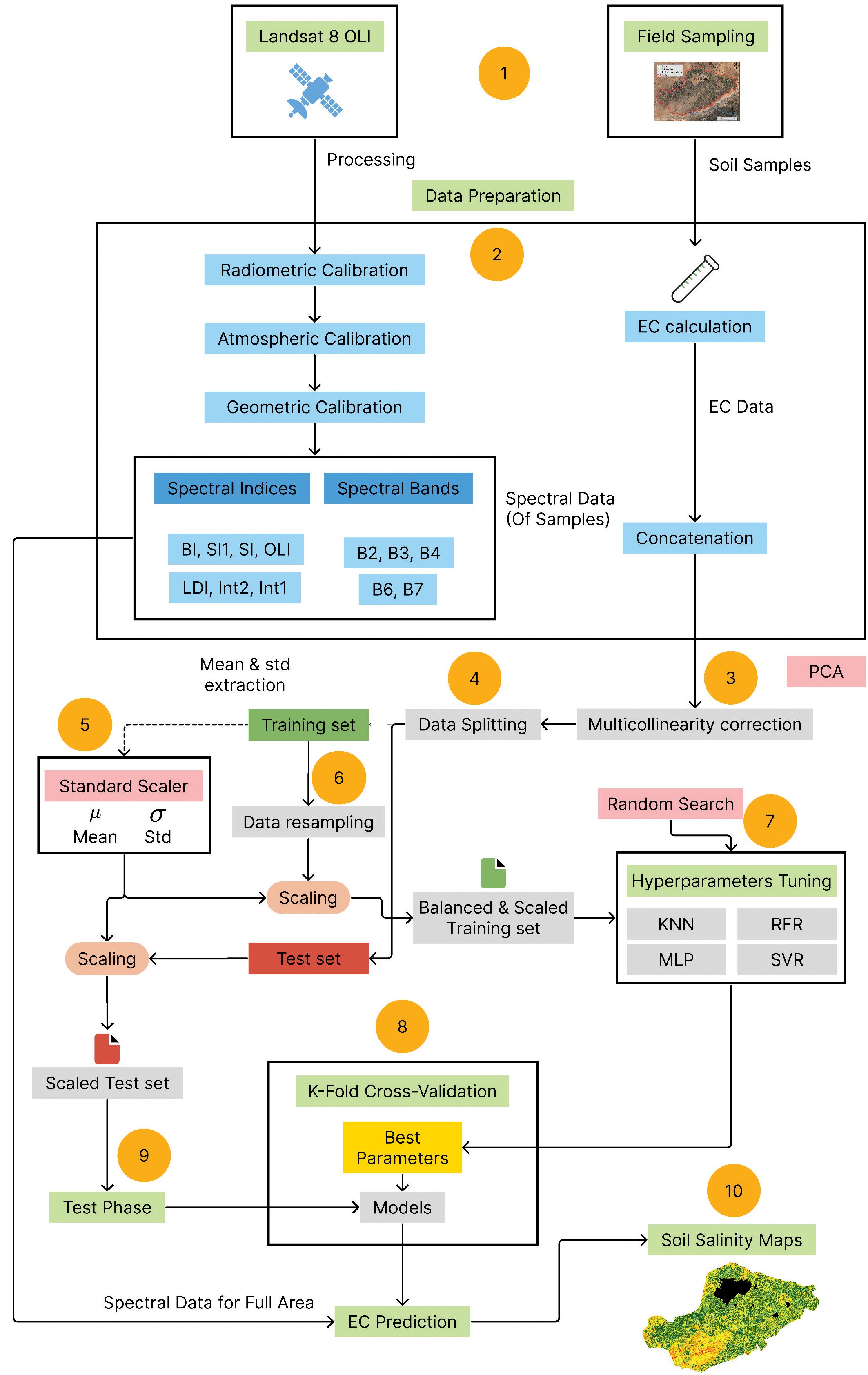
Figure 2. Flowchart detailing the workflow for soil salinity mapping, from data acquisition to map generation.

Concurrently, Landsat imagery acquired on November 12, 2021(cloud cover = 0.11%), downloaded from (https://earthexplorer.usgs.gov/, accessed on December, 1st 2021), and preprocessed in QGIS 2.18.0. The image has been radiometrically calibrated and atmospherically corrected using the Dark Object Subtraction (DOS) (23, 34). The data was geometrically corrected to align with the collected ground truth data, facilitating seamless integration for comparative analysis.

Furthermore, spectral bands spanning from the visible, including Blue (B2), Green (B3), and Red (B4), to the short-wave infrared wavelengths, SWIR1 (B6) and SWIR2 (B7), are used as recommended by previous studies (35, 36). Their efficiency in identifying and mapping salt-affected soils underscores their essential role in assessing soil degradation in both agricultural and natural landscapes. Spectral indices were calculated, including soil salinity indices (37, 38), intensity indices (39), brightness indices (38), and the land degradation index (LDI) (7, 40) (Supplementary Table S2, Supplementary Figure S1 in the Supplementary Material).

Data preprocessing was performed in a Visual Studio Code environment using the Python programming language, involving the application of resampling techniques to overcome class imbalances, scaling methods to normalize spectral and laboratory data, and principal component analysis (PCA) to address multicollinearity among predictor variables, and to enhance the stability and performance of the models. The first five principal components (PC1-PC5) were subsequently used as input variables for all ML models. This transformation ensured that all predictors were orthogonal, and representative of the main spectral variance associated with soil salinity.

Additionally, a systematic data-splitting approach has been applied, dividing the data into training (70%) and testing (30%) subsets, with 20 (folds) runs using different random seeds to assess model stability. It is worth noting that the resampling method was applied only to the training subset. The testing subset was left untouched to validate the models’ performance. The ML model’s performance was evaluated using three metrics: the coefficient of determination (R2), Mean Absolute Error (MAE), and Root Mean Square Error (RMSE). In each iteration, the metrics were calculated to determine the models’ performance and stability. Additionally, 95% Confidence Intervals (CI) for R² were also estimated to quantify the uncertainty of the models (41, 42). Additionally, statistical differences among models were evaluated using the Friedman test (43, 44), followed by the Nemenyi post-hoc test for pairwise comparisons (45). Once validated, the four ML models with median performance metrics were deployed to generate soil salinity maps, enabling a comparative spatial assessment of their predictive performance and providing valuable insights for sustainable land management.

2.3 Data resampling

Given the limited sample size characteristic of field campaigns in data-scarce regions, machine learning models are highly susceptible to overfitting and learning the noise in the data rather than the actual insights regarding the target variable. To mitigate this risk and enhance model robustness, a data augmentation strategy employing bootstrapping with noise is used (46). This technique involves resampling the original training data samples with replacement (bootstrapping), where the target variable (ECe) belongs to different intervals. Next, a small amount of random noise drawn from a Gaussian distribution was injected into the data. According to Aksoy et al. (15), the use of random oversampling techniques enables the model to learn a more generalizable function of the target variable, rather than memorizing individual data points.

2.4 Data standardization

The dataset was normalized using a standard-scaling method (Equation 1). The standardized values were subsequently rescaled to the interval of (–1, 1) to enhance numerical stability and facilitate the convergence of ML models, as recommended in previous studies (47, 48).

$\begin{array}{ll}{x}_{scaled}=\frac{x_i-x_{mean}}{\sigma }& (1)\end{array}$

where $x_{scaled}$ is the scaled variable, $x_i$ is the $i^{th}$ sample variable, $x_{mean}$ is the average value, and $\sigma$ is the standard deviation. The mean and standard deviation of the training set were computed before the resampling phase, and were used on the resampled training subset, as well as the testing subset.

2.5 Multicollinearity correction

Among the variables used, most spectral bands and indices are inherently correlated, and such multicollinearity can distort regression coefficients, inflate variance, and reduce the stability of predictive models (49). PCA addresses this issue by transforming the original set of correlated variables into a smaller number of orthogonal (uncorrelated) principal components, each representing a linear combination of the original features (50). In our case, we retained enough components to preserve up to 99% of the variance in the data, resulting in five non-collinear components that capture nearly all the information in the original data. This transformation not only enhances model stability and predictive performance but also mitigates the risk of overfitting that may arise when highly collinear predictors are used in ML algorithms (49).

2.6 Machine learning

The algorithms used in this research fall into the category of supervised ML algorithms. The ground truth corresponding to the samples was provided as input to the model during the calibration phase. Four ML models were implemented: KNN, SVR, RF, and MLP. In addition to being widely used in literature, these models use a learning approach to identify hidden patterns in the data and correlate the input and output variables (22, 51).

2.6.1 K-nearest neighbors

The KNN algorithm is designed for classification problems where the class of the sample is determined based on the majority class of its n closest neighbors (52, 53). The number of neighbors is the main parameter in this algorithm (54). In the case of regression, the average values of the closest neighbors are taken as the prediction.

2.6.2 Support vector regressor

Similarly, SVM is dedicated to classification tasks; however, its regression version, SVR, attempts to discover a hyperplane optimally fitting the data points in a continuous space (55). The input variables are mapped into a high-dimensional space of features, and the hyperplane is found that maximizes the distance between the hyperplane and the nearest data points while minimizing the error of prediction (56).

2.6.3 Random forest

RF algorithm consists of several decision trees, each of which is trained on a random subset of the data, and computing the outcome (57). The outputs are then aggregated into a final output value (33, 58). The RF classifier takes the majority votes of the trees’ predictions, unlike the regression version, which tends to average the trees’ predictions and assigns the average to the predicted instance.

2.6.4 Multi-layer perceptron

MLP is a type of Artificial Neural Networks (ANNs) used for function approximation, pattern recognition, and classification tasks (59). They are known for their ability to capture complex relationships in data by learning through multiple computation layers (60).

Furthermore, although each model has different parameters, it is optimal to determine the best hyperparameters for training the models. For this purpose, we employed a random-search technique (23, 61). This later enabled us to examine the performance of the models under the influence of various sets of hyperparameters. Additionally, it is noteworthy that we launched hyperparameter tuning under a range of random seeds to eliminate the bias introduced by randomness. Table 1 lists the different parameter sets for each algorithm, along with the optimal parameters in each case.

Table 1

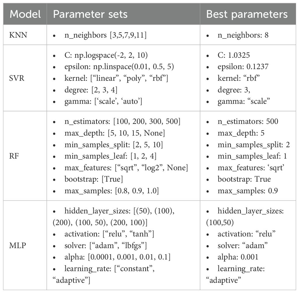
Table 1. Search space and the best hyperparameters.

2.7 Evaluation metrics

To validate the performance of the models, three evaluation metrics were used, namely: R²,MAE, and RMSE, as described by Equations 2–4, respectively.

$\begin{array}{ll}{R}^2=1-\frac{{\sum }_{i=1}^n{(y_i-{\widehat{y}}_i)}^2}{{\sum }_{i=1}^n{(y_i-\underset{\_}{y})}^2}& (2)\end{array}$

$\begin{array}{ll}MAE=\frac{1}{n}{\sum }_{i=1}^n❘y_i-{\widehat{\text{y}}}_i❘ & (3)\end{array}$

$\begin{array}{ll}RMSE=\sqrt{\frac{1}{n}({\sum }_{n=1}^n{(y_i-{\widehat{y}}_i)}^2}& (4)\end{array}$

Where $y_i$ is the observed value, ${\widehat{y}}_i$ is the predicted value, $\underset{¯}{y }$is the mean value, and $n$ s the number of samples in the testing dataset.

3 Results

3.1 Descriptive statistics of ECe and predictor correlations

The statistical analysis parameters for the target variable (ECe) and independent variables are illustrated in Figure 3. The ECe values in the study area ranged from 0.84 to 10.28 dS/m, with a standard deviation (Std) of 2.29 dS/m, reflecting considerable variation in soil salinity levels. Spatially, high EC values were concentrated downstream (southwest), while lower values were observed towards the northeast region.

Figure 3

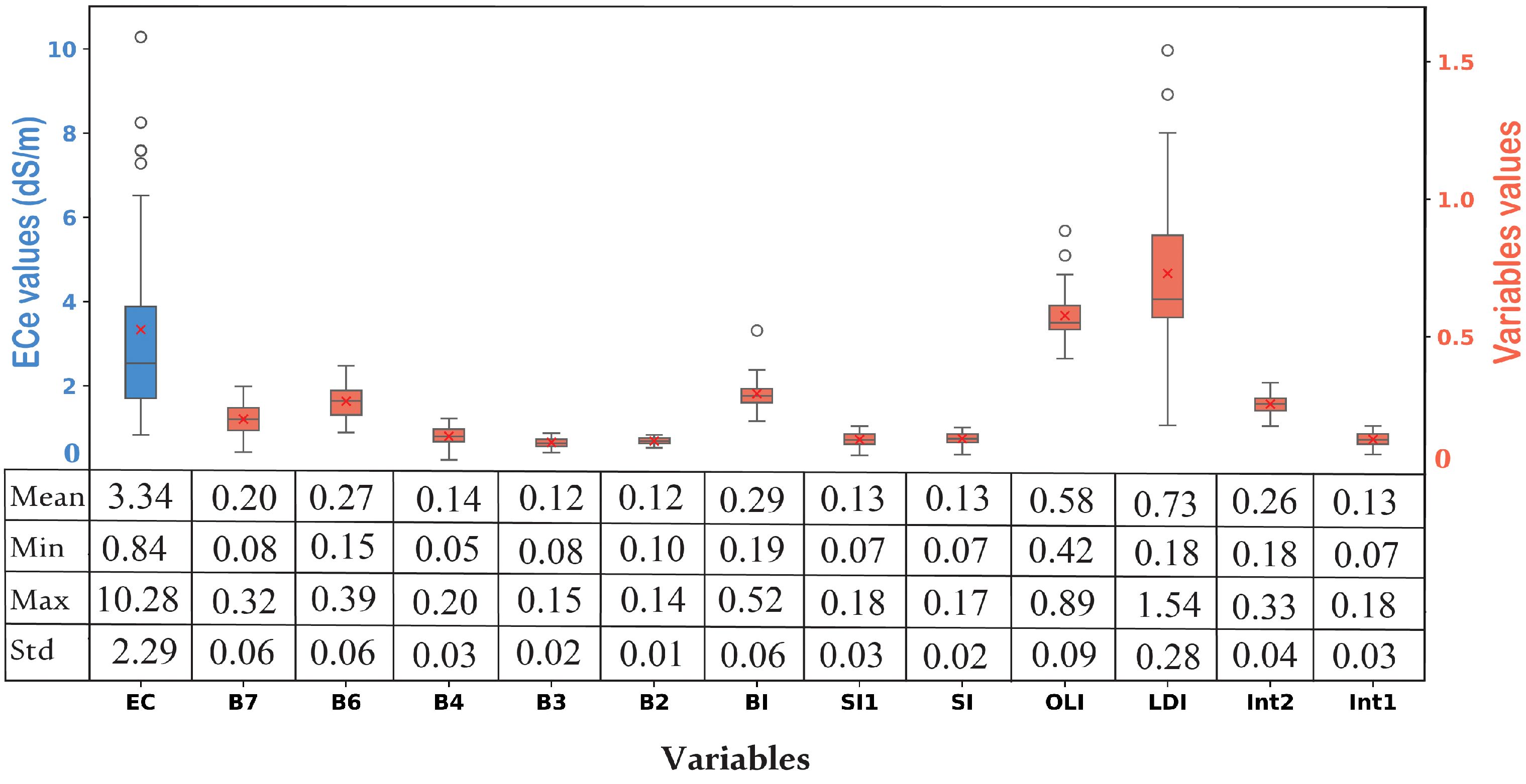
Figure 3. Boxplots of descriptive statistics for ECe and predictor variables, including spectral bands and indices.

Derived spectral bands and indices varied between 0 and 1.5. Among them, LDI and OLI showed the greatest variability, with a Std of 0.28 and 0.09, respectively. Meanwhile, other variables exhibited lower variability, with a Std ranging between 0.01 and 0.06.

The correlation matrix (Figure 4) revealed a strong positive relationship between the target variable EC and OLI and LDI, as well as bands 7 and 6, indicating their potential relevance to salinity variability. Conversely, BI and Int2 showed weak correlation with ECe, suggesting limited direct predictive value. However, several predictors exhibited strong intercorrelations, particularly Int1 with SI, SI1, B4, B3, B2, B7, and B6, indicating substantial multicollinearity among the spectral variables.

Figure 4

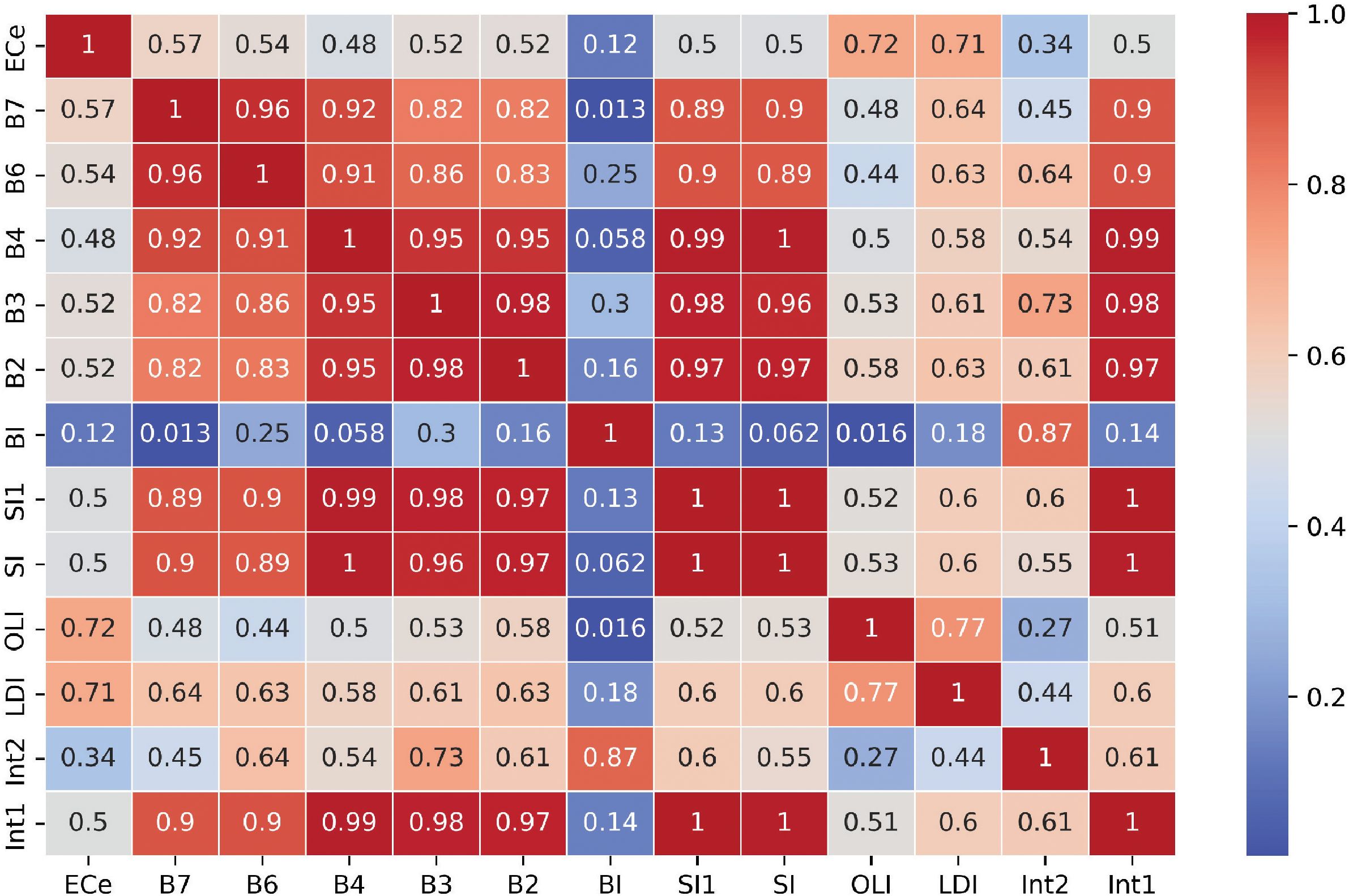
Figure 4. Correlation matrix among ECe and predictor variables, including spectral bands and indices.

Given these interrelationships, PCA was applied to standardized predictors, transforming the original 13 correlated variables into orthogonal principal components (PCs). The loading pattern (Supplementary Figure S2a) indicates that PC1 carries broadly uniform positive contributions across predictors, PC2 is dominated by BI (≈0.75), PC3 by OLI-SI/LDI/OLI (≈0.58–0.59), PC4 by B6 (≈0.53) with a negative OLI contribution (≈−0.41), and PC5 by LDI (≈0.70) with a negative OLI contribution (≈−0.60). The scree and cumulative variance plots (Supplementary Figure S2–c) indicate that PC1–PC5 account for approximately 99% of the total variance.

3.2 Models performance

Model training was performed using 70% (80 samples) of the dataset, with the remaining 30% (11 samples) reserved for testing. A comparison of the predicted and measured ECe values revealed that the models exhibit comparable performances during the training phase (Figure 5, Table 2). As previously mentioned, the models that yielded median scores were retained for performance representation. The KNN model yielded the lowest accuracy (R² = 0.91), while the RF, SVR, and MLP models achieved the highest accuracy (R² = 0.99). Overall, the predicted values generally aligned well with the measured ECe values, indicating satisfactory model training (Figure 6).

Figure 5

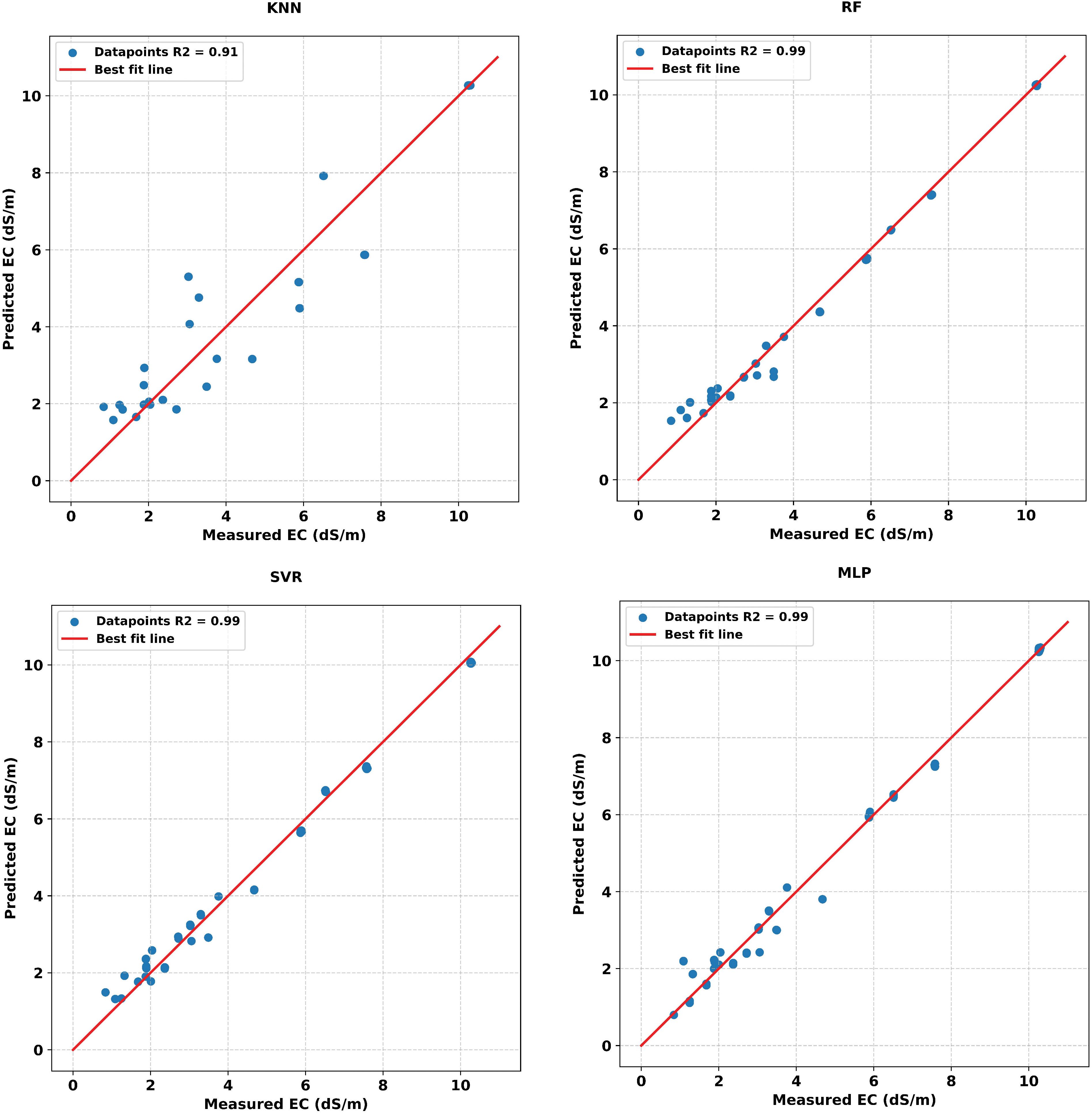
Figure 5. Comparison between measured and predicted EC values for the training dataset using for machine learning models: KNN, RF, SVR, and MLP.

Table 2

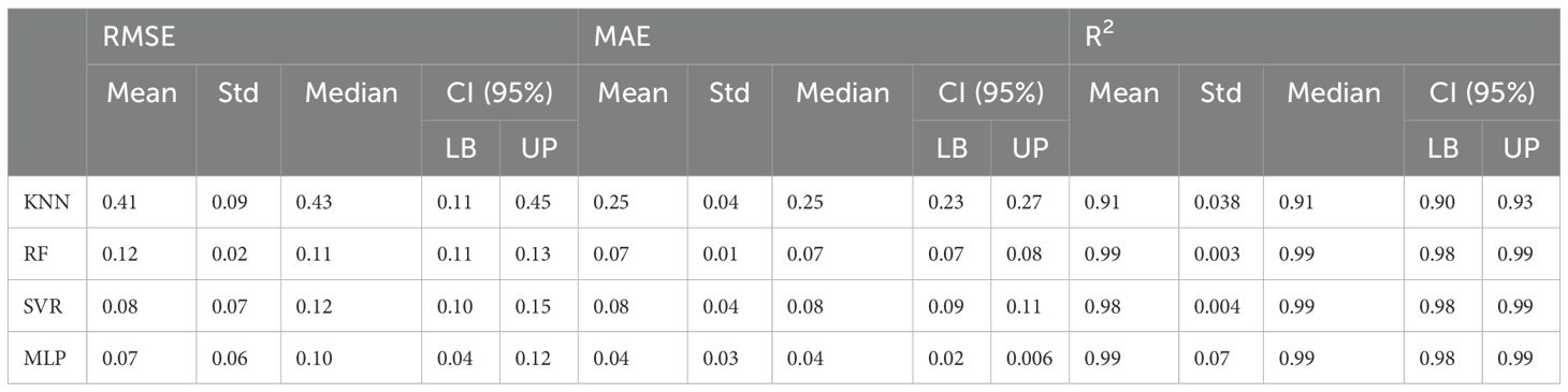
Table 2. Evaluation of metrics for the train set.

Figure 6

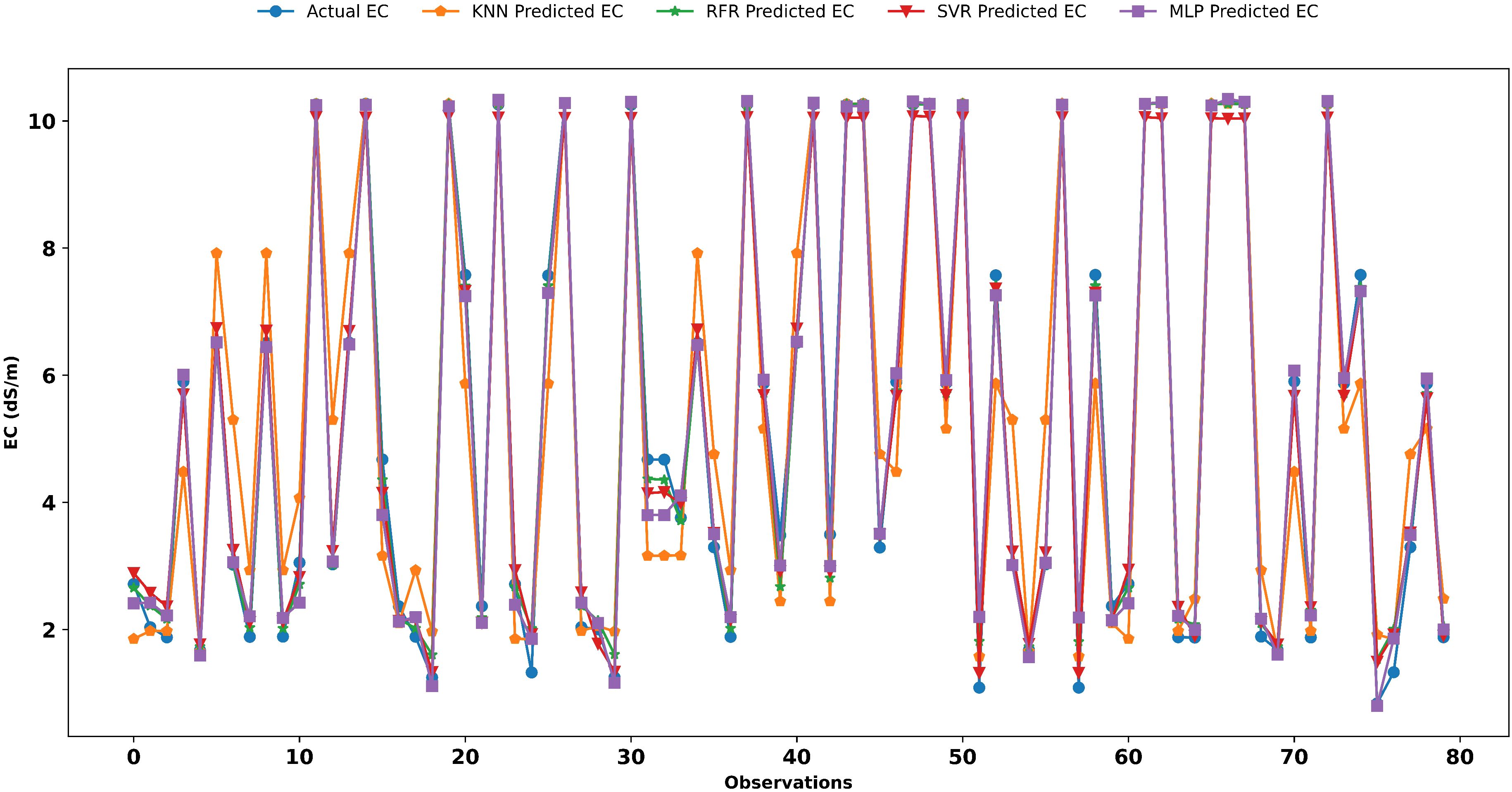
Figure 6. Comparison of observed EC with model predictions acoss 80 training observations.

However, during the testing phase, performance differences become more evident (Table 3). The RF and MLP models resulted in relatively low accuracy (R² = 0.53; RMSE = 0.75 dS/m; and R² = 0.45; RMSE = 0.90 dS/m, respectively), failing to generalize to the independent test dataset, indicating overfitting, especially in the case of MLP. In contrast, the SVR model exhibited moderate predictive accuracy, with an R² of 0.59 and an RMSE of 0.62 dS/m, suggesting slight overfitting (Figure 7). On the other hand, KNN achieved the best results, with an R² score of 0.76 and an RMSE of 0.40 dS/m.

Table 3

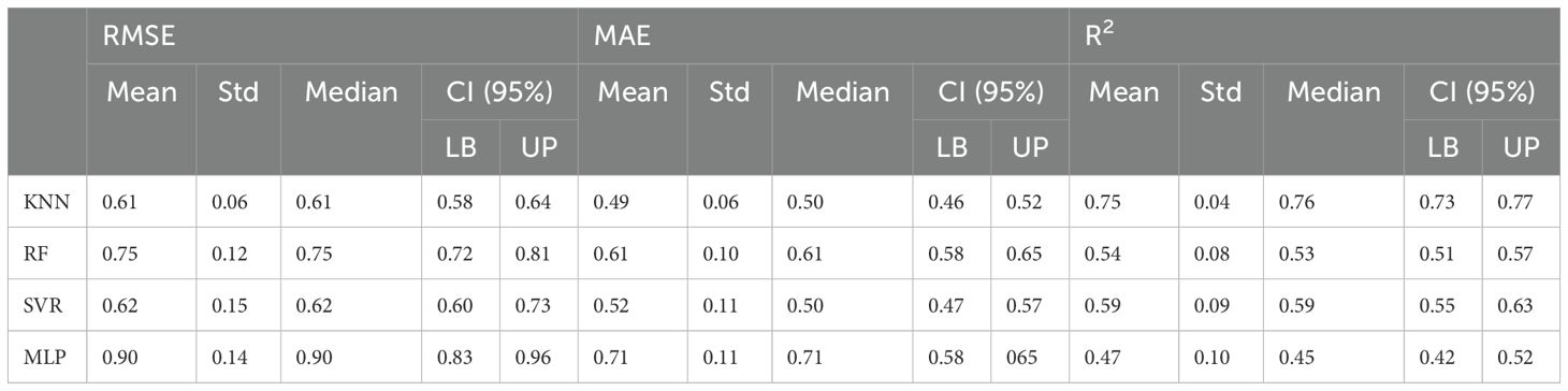
Table 3. Evaluation of metrics for the test set.

Figure 7

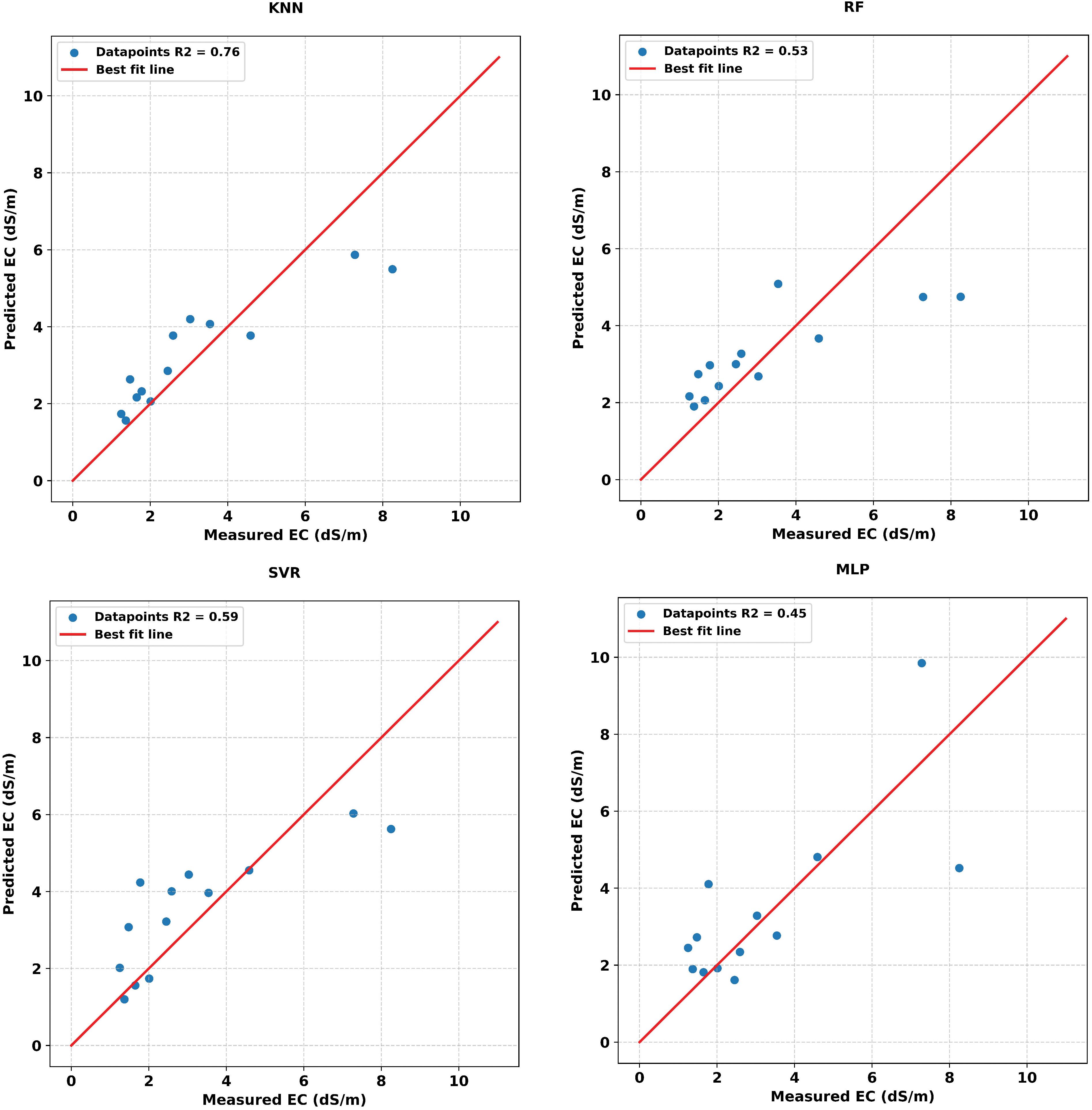
Figure 7. Comparison between measured and predicted EC values for the testing dataset using for machine learning models: KNN, RF, SVR, and MLP.

Although the overall results are relatively low (except for KNN), the models still follow the general pattern of EC variation and predict the peaks and troughs observed in the measured data (Figure 8). Additionally, sudden variations in EC lead to predictions that overshoot or undershoot the target value; these examples occur around the third (sudden decrease), fourth (sharp increase), and fifth peaks. These peaks were not reproduced by any of the models, with a greater overestimation and underestimation in MLP and RF, respectively. On the much smoother datapoints, the models tend to closely follow the EC data, with KNN producing the best visual results (8th to 12th datapoints). At the same time, MLP and SVR exhibit erratic behavior (9th-12th datapoints). Generally, the chart shows that while all models effectively capture the temporal dynamics of EC, MLP and SVR exhibit significant instability. In contrast, KNN provides the most visually consistent predictions with the observed measurements.

Figure 8

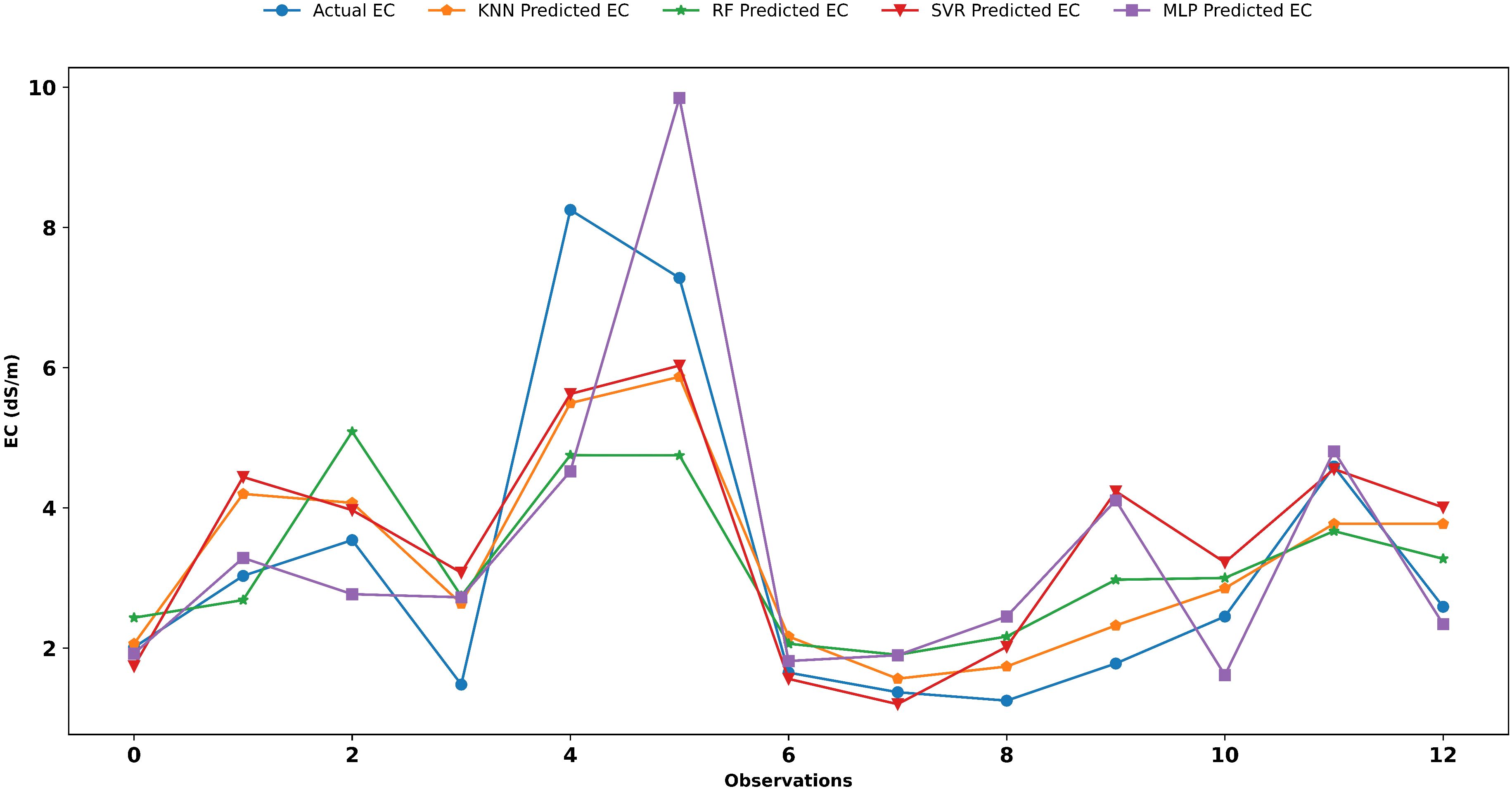
Figure 8. Comparison of observed EC with model predictions acoss 11 testing observations.

To strengthen the comparative evaluation of the tested models, additional statistical analyses were performed. First, the 95% CI for R² was calculated to assess the variability and robustness of model performance (Table 4). Based on results from k-fold experiments with a 20-fold split (Figure 9), the KNN model achieved the highest predictive accuracy, with a mean R² of 0.75 (95% CI: 0.73–0.77). Conversely, the MLP recorded the lowest performance (mean R² = 0.45, CI: 0.42–0.52). To assess whether differences among models were statistically significant, a Friedman test was conducted, yielding a χ²(3) statistic of 22.90 and a p-value of 0.0 (<0.05), confirming substantial differences in performance rankings. A subsequent Nemenyi post-hoc test revealed that the performances of RF, SVR, and MLP were statistically comparable (p > 0.05), with SVR and MLP being marginally different (p=0.04). In contrast, KNN differed significantly from the other models (p < 0.05) (Table 4). These findings reinforce the conclusion that KNN indeed performs best among the models used for soil salinity in the study area.

Table 4

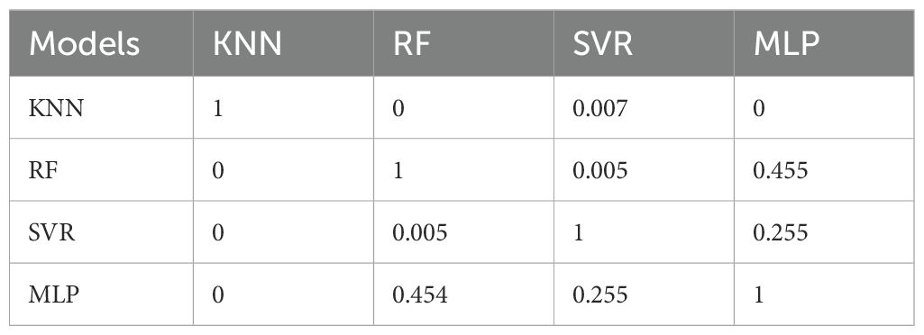
Table 4. Nemenyi post-hoc test p-values for pairwise model comparisons.

Figure 9

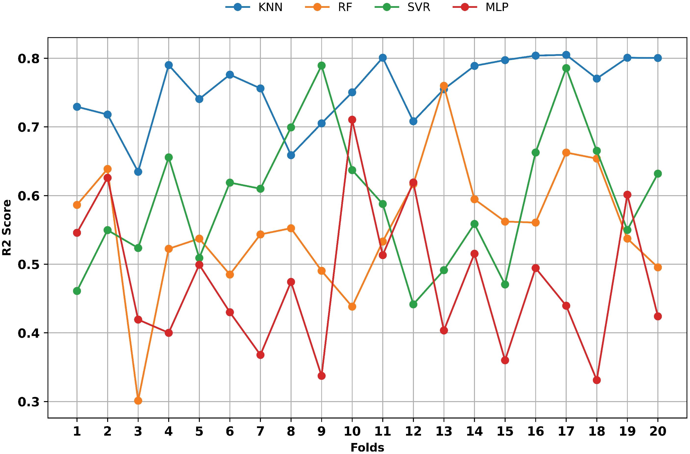
Figure 9. R² performance across 20-fold cross-validation on the test splits for four regression models predicting EC.

3.3 Spatial salinity distribution

The maps generated (Figure 10) show a progressive increase in soil salinity from upstream to downstream (southwest). The spatial analysis of soil salinity classes shows distinct predictive behaviors under different ML models (Figure 11). The KNN classified the most significant portion of areas as moderately saline (49%) and showed a substantial share in non-saline soils (20%), but also produced the highest proportion of strongly saline (8.4%) and extremely saline (0.6%) areas. SVR and RF yielded comparable distributions, with moderately saline classes covering 41% and 32% of the regions, respectively, while strongly saline soils represented 6% (SVR) and 10% (RF), and extremely saline areas remained limited (1% and 0.8%). In contrast, MLP predicted the highest proportion of slightly saline soils (48.5%) and a similar share of moderately saline areas (30%), with only 1.4% being strongly saline. Overall, while KNN provided the most balanced and accurate classification, MLP and RF emphasized slightly to moderately saline conditions, and SVR maintained intermediate estimates across classes.

Figure 10

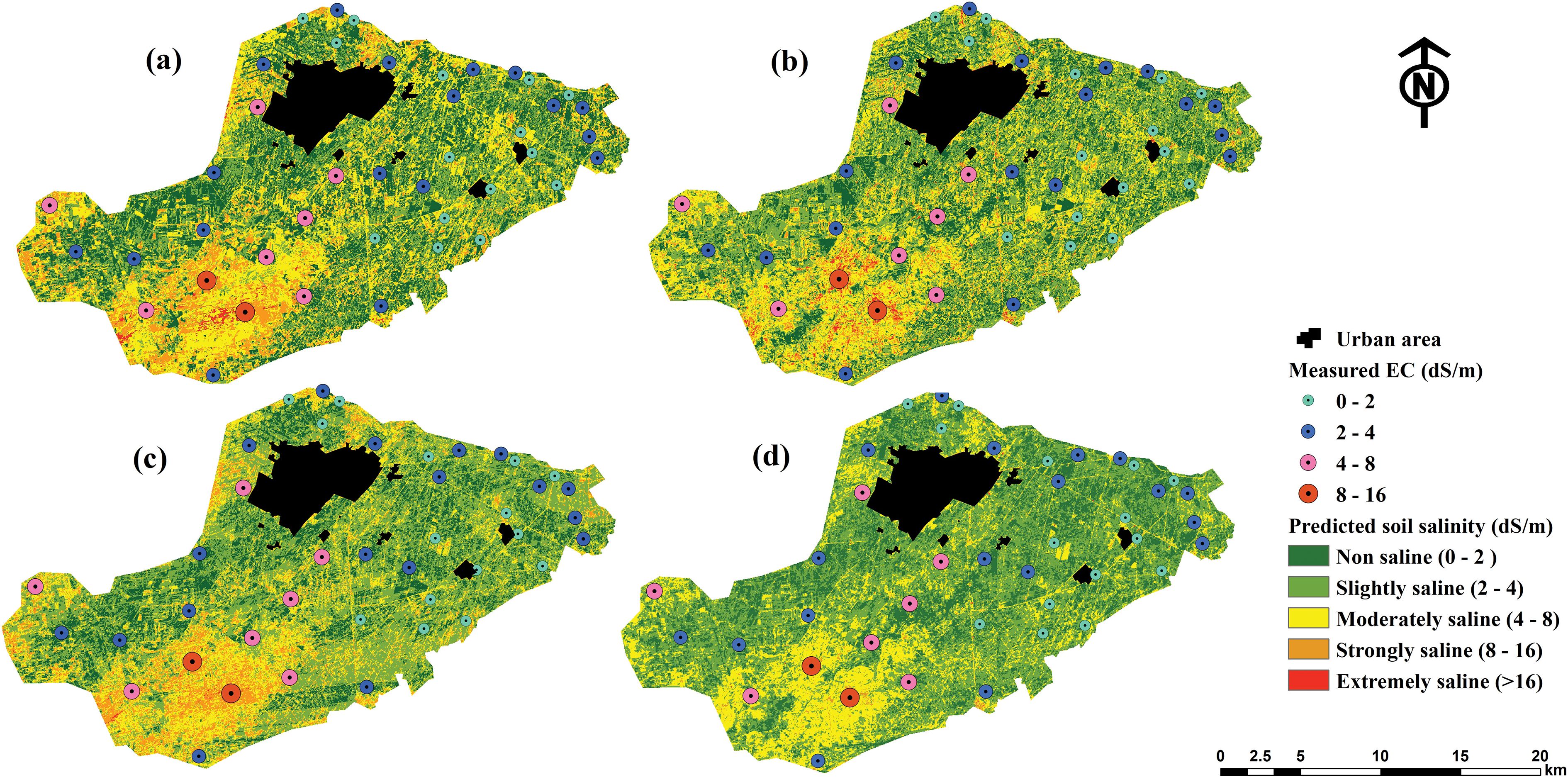
Figure 10. Soil salinity maps generated using KNN (a), SVR (b), RF (c), and MLP (d).

Figure 11

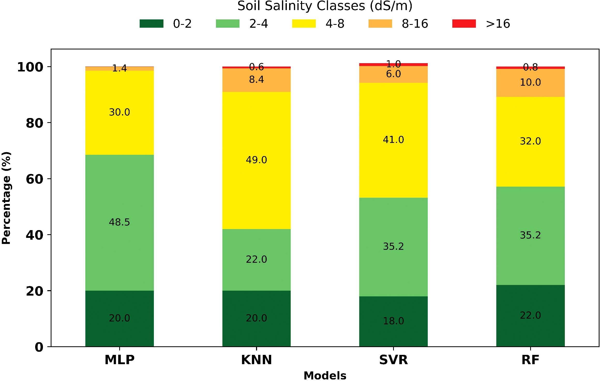
Figure 11. Percentage of soil salinity classes predicted by each model.

4 Discussion

Remote sensing combined with ML has been applied extensively for soil salinity assessment in diverse environments. Ivushkin et al. (33) reported that CART achieved a higher accuracy (70%) than SVM and RF using thermal data. Ge et al. (62) demonstrated the strong predictive ability of the gradient boosting regression tree (GBRT) with Sentinel-2 MSI and environmental covariates(R² = 0.88; RMSE = 6.33 dS/m). Kaplan et al. (63) found that the instance-based learning with parameter k (IBK) outperformed RF and linear regression in arid regions. In Morocco, numerous studies have explored the mapping of salt-affected soils using spectral indices and statistical models. Lhissou, et al. (64) obtained R² = 0.90 in the Tadla plain by combining satellite data with field EC measurements. El hafyani et al. (65) and Rafik et al. (66) reported high predictive power in the Tafilalt plain through regression-based approaches. Ait Lahssaine et al. (67) documented increasing salinization in Rheris oases between between1990 and 2022. These studies illustrate the value of remote sensing but generally rely on limited predictor sets.

This study contributes by integrating multiple variables within an ML framework to assess soil salinity in the Béni Amir sub-perimeter. Correlation analysis (Figure 4) revealed the strongest associations between Ece and OLI-SI and LDI, followed by SWIR-related bands (B7, B6), whereas BI and Int2 show weak relationships. The original predictors were then summarized into orthogonal principal components (Supplementary Figure S2a) to mitigate collinearity while retaining salinity-related variance. Consequently, interpretation emphasizes how salinity information is captured by the leading PCs rather than by any single raw predictor, with the strongest Ece associations concentrated in the first components.

Among the tested models, KNN demonstrated the highest predictive accuracy (mean R² = 0.75; RMSE = 0.61 dS/m). The SVR exhibits competitive performance (mean R² = 0.59; RMSE = 0.62 dS/m). MLP and RF performed similarly, with an R² of 0.47 and 0.54 and RMSEs of 0.90 and 0.75 dS/m, respectively. Confidence-interval analysis further corroborated the superiority and robustness of KNN, as evidenced by its narrow R² interval (± 0.03 around the mean).

The salinity maps exhibit a transparent gradient, with elevated EC concentrated downstream (southwest) and lower values in the upstream (northeast). This pattern follows the regional hydraulic flow as reported by El Harti et al. (8). Furthermore, the spatial distribution of soil salinity in sub-perimeter of Béni Amir is further reinforced by topographic effects promoting solute accumulation in low-lying areas (68), land cover dynamics influencing salt inputs and leaching (11), and climatic conditions enhancing evaporite concentration during dry periods (10).

Although all models reproduced the main gradient, KNN yielded the most spatially coherent predictions with realistic transitions between classes. Considering both predictive accuracy and spatial plausibility, the KNN-derived map is the most reliable product for operational decision-making in Béni Amir.

Operational guidance based on the KNN map targets interventions by salinity class. For strongly and extremely saline soils, actions include drainage rehabilitation, controlled leaching, and shifting to salt-tolerant crops or intercropping; gypsum application is advised for sodicity. In moderately saline soils, preventive strategies involve selecting moderately tolerant cultivars, using intercropping, pressurized irrigation with leaching, and routine EC monitoring. For low-salinity soils, maintaining optimized irrigation, periodic testing, and balanced fertilization are recommended. The implementation prioritizes KNN-identified hotspots, conducting field verification before making significant investments, thereby offering a robust, site-specific framework for salinity management.

While several studies have highlighted the strong performance of tree-based and ensemble learners, our results indicate that KNN achieved the highest predictive accuracy for soil salinity in this context. This contrasts with reports where RF excelled, for example Haq et al. (17) in Punjab Province, Pakistan (R² of 0.94; RMSE of 1.89) and with findings that favored RF over ANN and SVM in environmental applications (23). Ensemble methods such as AdaBoost and XGBoost have also shown promise for salinity prediction (69, 70), particularly with multisource integration. Nonetheless, the superior performance of KNN in our study suggests that instance-based learning can be highly competitive when local neighborhood structure is informative.

Overall, algorithm selection materially influences both predictive accuracy and the spatial depiction of salinity. Integration of remote sensing with ML, supported by PCA-based predictor representation, improved mapping precision in Béni Amir and enabled robust hotspot identification. The KNN-derived map provides the most reliable basis for management, informing prioritized drainage upgrades, calibrated leaching, irrigation-water quality management, and the deployment of salt-tolerant cultivars and intercropping systems in areas with high salinity concentrations.

Although ML combined with satellite data proved effective for salinity prediction, several challenges remain. Model performance is sensitive to the selection of input variables, necessitating careful calibration with field ECe data. Importantly, the relatively limited field dataset (n = 43) constrains model generalization, as most ML algorithms require larger samples to capture spatial variability and can increase the risk of overfitting, potentially degrading performance when extrapolated to new conditions. Advances in sensor technology necessitate a more comprehensive assessment of optimal spectral bands and index combinations. Incorporating additional environmental parameters such as land use, climate, topography, and soil properties could improve robustness. Future research should also include quantitative uncertainty assessments (e.g., sensitivity analyses) to enhance model reliability and evaluate the approach’s transferability to other irrigated systems. Beyond data-driven models, future directions should explore physics-informed neural networks (PINNs). In their simplest form, PINNs can be implemented as multilayer perceptrons with modified loss functions that enforce known physical constraints (e.g., mass balance, salinity transport relationships), thereby improving plausibility and stability under data scarcity and expanding generalizability across regions and seasons.

5 Conclusion

Soil salinization is a significant contributor to land degradation in arid and semi-arid regions. This study demonstrated the effectiveness of ML for predicting soil salinity in the Béni Amir sub-perimeter of the Tadla Plain. The KNN achieved the highest accuracy (mean R² = 0.75; RMSE = 0.61 dS/m), while the SVR and RF performed competitively. On the other hand, the MLP performed least effectively. Predicted maps revealed a downstream accumulation of salinity, primarily due to saline irrigation water, inadequate drainage, and intensive farming practices.

These findings highlight the potential of ML models, combined with satellite-derived predictors, to provide reliable and scalable tools for monitoring soil salinity in irrigated agroecosystems. The proposed framework offers valuable support for sustainable land management and irrigation planning. Future research is needed on drivers and the approach, integrating socio-economic drivers, and assessing the cost-effectiveness of land reclamation strategies.

Data availability statement

The datasets generated and/or analyzed during the current study are available from the corresponding author upon reasonable request.

Author contributions

AC: Writing – original draft, Visualization, Formal analysis, Writing – review & editing, Software, Methodology, Data curation, Investigation. HA-I: Writing – review & editing, Investigation, Writing – original draft, Methodology, Software, Visualization, Formal analysis. SH: Software, Conceptualization, Writing – original draft, Visualization, Formal analysis. MC: Validation, Writing – review & editing, Resources, Supervision, Data curation, Investigation, Conceptualization. MN: Investigation, Writing – review & editing, Supervision, Validation, Data curation. MH: Supervision, Conceptualization, Writing – review & editing, Methodology, Project administration, Validation, Resources. ME: Conceptualization, Methodology, Validation, Writing – review & editing, Investigation, Formal analysis, Writing – original draft, Visualization. YA: Supervision, Writing – review & editing, Validation, Resources, Project administration. LB: Resources, Formal analysis, Writing – review & editing, Supervision, Visualization, Methodology, Conceptualization, Funding acquisition, Validation.

Funding

The author(s) declare that no financial support was received for the research, and/or publication of this article.

Acknowledgments

The authors thank the Moroccan Ministry of Higher Education, Scientific Research and Innovation, the OCP Foundation, the UM6P, and the CNRST, who supported this work through the APRD research program (GEANTech).

Conflict of interest

The authors declare that the research was conducted in the absence of any commercial or financial relationships that could be construed as a potential conflict of interest.

Generative AI statement

The author(s) declare that no Generative AI was used in the creation of this manuscript.

Any alternative text (alt text) provided alongside figures in this article has been generated by Frontiers with the support of artificial intelligence and reasonable efforts have been made to ensure accuracy, including review by the authors wherever possible. If you identify any issues, please contact us.

Publisher’s note

All claims expressed in this article are solely those of the authors and do not necessarily represent those of their affiliated organizations, or those of the publisher, the editors and the reviewers. Any product that may be evaluated in this article, or claim that may be made by its manufacturer, is not guaranteed or endorsed by the publisher.

Supplementary material

The Supplementary Material for this article can be found online at: https://www.frontiersin.org/articles/10.3389/fsoil.2025.1653400/full#supplementary-material

References

1. Ait Brahim Y, Benkaddour A, Agoussine M, Ait Lemkademe A, Yacoubi LA, and Bouchaou L. Origin and salinity of groundwater from interpretation of analysis data in the mining area of Oumjrane, Southeastern Morocco. Environ Earth Sci. (2015) 74:4787–802. doi: 10.1007/s12665-015-4467-7

Crossref Full Text | Google Scholar

2. El-Azhari A, Ait Brahim Y, Barbecot F, Hssaisoune M, Berrouch H, Laamrani A, et al. Evaluating groundwater salinity patterns and spatiotemporal dynamics in complex endorheic aquifer systems. Sci Total. Environ. (2025) 994:180055. doi: 10.1016/j.scitotenv.2025.180055

PubMed Abstract | Crossref Full Text | Google Scholar

3. Omuto CT, Kome GK, Ramakhanna SJ, Muzira NM, Ruley JA, Jayeoba OJ, et al. Trend of soil salinization in Africa and implications for agro-chemical use in semi-arid croplands. Sci Total. Environ. (2024) 951:175503. doi: 10.1016/j.scitotenv.2024.175503

PubMed Abstract | Crossref Full Text | Google Scholar

4. FAO. Global map of salt-affected soils. (2021) (Rome, Italy: Food and Agriculture Organization (FAO)).

Google Scholar

5. Negacz K, Malek Ž., de Vos A, and Vellinga P. Saline soils worldwide: Identifying the most promising areas for saline agriculture. J Arid. Environ. (2022) 203:104775. doi: 10.1016/j.jaridenv.2022.104775

Crossref Full Text | Google Scholar

6. Singh A. Soil salinization management for sustainable development: A review. J Environ Manage. (2021) 277:111383. doi: 10.1016/j.jenvman.2020.111383

PubMed Abstract | Crossref Full Text | Google Scholar

7. Chaaou A, Chikhaoui M, Naimi M, Miad AKE, Bokoye AI, Ennasr MS, et al. Potential of land degradation index for soil salinity mapping in irrigated agricultural land in a semi-arid region using Landsat-OLI and Sentinel-MSI data. Environ Monit Assess. (2024) 196:843. doi: 10.1007/s10661-024-13030-1

PubMed Abstract | Crossref Full Text | Google Scholar

8. El Harti A, Lhissou R, Chokmani K, Ouzemou J, Hassouna M, Bachaoui EM, et al. Spatiotemporal monitoring of soil salinization in irrigated Tadla Plain (Morocco) using satellite spectral indices. Int J Appl Earth Obs. Geoinformation. (2016) 50:64–73. doi: 10.1016/j.jag.2016.03.008

Crossref Full Text | Google Scholar

9. Ennaji W, Barakat A, Karaoui I, El Baghdadi M, and Arioua A. Remote sensing approach to assess salt-affected soils in the north-east part of Tadla plain, Morocco. Geol Ecol Landsc. (2018) 2:22–8. doi: 10.1080/24749508.2018.1438744

Crossref Full Text | Google Scholar

10. Chaaou A, Chikhaoui M, Naimi M, El Miad AK, Achemrk A, Seif-Ennasr M, et al. Mapping soil salinity risk using the approach of soil salinity index and land cover: a case study from Tadla plain, Morocco. Arab. J Geosci. (2022) 15:722. doi: 10.1007/s12517-022-10009-5

Crossref Full Text | Google Scholar

11. El Hamdi A, Morarech M, El Mouine Y, Rachid A, El Ghmari A, Yameogo S, et al. Sources of spatial variability of soil salinity: the case of Beni Amir irrigated command areas in the Tadla Plain, Morocco. Arid. Land. Res Manage. (2022), 1–20. doi: 10.1080/15324982.2022.2026531

Crossref Full Text | Google Scholar

12. Scudiero E, Corwin DL, Anderson RG, and Skaggs TH. Moving forward on remote sensing of soil salinity at regional scale. Front Environ Sci. (2016) 4:65. doi: 10.3389/fenvs.2016.00065

Crossref Full Text | Google Scholar

13. Gorji T, Sertel E, and Tanik A. Monitoring soil salinity via remote sensing technology under data scarce conditions: A case study from Turkey. Ecol Indic. (2017) 74:384–91. doi: 10.1016/j.ecolind.2016.11.043

Crossref Full Text | Google Scholar

14. Abuelgasim A and Ammad R. Mapping soil salinity in arid and semi-arid regions using Landsat 8 OLI satellite data. Remote Sens. Appl Soc Environ. (2019) 13:415–25. doi: 10.1016/j.rsase.2018.12.010

Crossref Full Text | Google Scholar

15. Aksoy S, Sertel E, Roscher R, Tanik A, and Hamzehpour N. Assessment of soil salinity using explainable machine learning methods and Landsat 8 images. Int J Appl Earth Obs. Geoinformation. (2024) 130:103879. doi: 10.1016/j.jag.2024.103879

Crossref Full Text | Google Scholar

16. Bannari A and Al-Ali ZM. Assessing climate change impact on soil salinity dynamics between 1987–2017 in arid landscape using landsat TM, ETM+ and OLI data. Remote Sens. (2020) 12:2794. doi: 10.3390/rs12172794

Crossref Full Text | Google Scholar

17. Haq YU, Shahbaz M, Asif S, Ouahada K, and Hamam H. Identification of soil types and salinity using MODIS terra data and machine learning techniques in multiple regions of Pakistan. Sensors. (2023) 23:8121. doi: 10.3390/s23198121

PubMed Abstract | Crossref Full Text | Google Scholar

18. Liu Y, Han X, Zhu Y, Li H, Qian Y, Wang K, et al. Spatial mapping and driving factor Identification for salt-affected soils at continental scale using Machine learning methods. J Hydrol. (2024) 639:131589. doi: 10.1016/j.jhydrol.2024.131589

Crossref Full Text | Google Scholar

19. Wang W and Sun J. Estimation of soil salinity using satellite-based variables and machine learning methods. Earth Sci Inform. (2024) 17:5049–61. doi: 10.1007/s12145-024-01467-4

Crossref Full Text | Google Scholar

20. Wang J, Ding J, Yu D, Teng D, He B, Chen X, et al. Machine learning-based detection of soil salinity in an arid desert region, Northwest China: A comparison between Landsat-8 OLI and Sentinel-2 MSI. Sci Total. Environ. (2020) 707:136092. doi: 10.1016/j.scitotenv.2019.136092

PubMed Abstract | Crossref Full Text | Google Scholar

21. Fu Y, Wang P, Cao W, Fu S, Zhang J, Li X, et al. Long-term assessment of soil salinization patterns in the yellow river delta using landsat imagery from 2003 to 2021. Land. (2024) 14:24. doi: 10.3390/land14010024

Crossref Full Text | Google Scholar

22. Naimi S, Ayoubi S, Zeraatpisheh M, and Dematte JAM. Ground observations and environmental covariates integration for mapping of soil salinity: A machine learning-based approach. Remote Sens. (2021) 13:4825. doi: 10.3390/rs13234825

Crossref Full Text | Google Scholar

23. Thangarasu T, Mengash HA, Allafi R, and Mahgoub H. Spatial prediction of soil salinity: Remote sensing and machine learning approach. J South Am Earth Sci. (2025) 156:105440. doi: 10.1016/j.jsames.2025.105440

Crossref Full Text | Google Scholar

24. Silatsa FBT and Kebede F. A quarter century experience in soil salinity mapping and its contribution to sustainable soil management and food security in Morocco. Geoderma Reg. (2023) 34:e00695. doi: 10.1016/j.geodrs.2023.e00695

Crossref Full Text | Google Scholar

25. Baite W, Boukdir A, and Baite M. Integrated management of irrigation water in the irrigated perimeter of Tadla (Morocco) and involvement of farmers in the aquifer contract. In: AIP conference proceedings. Morocco: AIP Publishing LLC (2021). p. 020043.

Google Scholar

26. Jabour H and Nakayama K. Basin modeling of Tadla basin, Morocco, for hydrocarbon potential. AAPG Bull. (1988) 72:1059–73. doi: 10.1306/703C97BC-1707-11D7-8645000102C1865D

Crossref Full Text | Google Scholar

27. Oumenskou H, El Baghdadi M, Barakat A, Aquit M, Ennaji W, Karroum LA, et al. Multivariate statistical analysis for spatial evaluation of physicochemical properties of agricultural soils from Beni-Amir irrigated perimeter, Tadla plain, Morocco. Geol Ecol Landsc. (2019) 3:83–94. doi: 10.1080/24749508.2018.1504272

Crossref Full Text | Google Scholar

28. Oussaoui S, Boudhar A, Hadri A, Lebrini Y, Houmma IH, Karaoui I, et al. Mapping drought severity impact on arboriculture systems over Tadla and lower Tassaout plains in Morocco using Sentinel-2 data and machine learning approaches. Geocarto Int. (2025) 40:2471104. doi: 10.1080/10106049.2025.2471104

Crossref Full Text | Google Scholar

29. Mouaddine A, Barakat A, Hajaj S, Mosaid H, Bouzekraoui H, Bni Z, et al. Predicting and mapping soil saturated hydraulic conductivity in the Beni Moussa irrigated perimeter (Tadla Plain, Morocco) using Random Forest machine learning model. Model Earth Syst Environ. (2025) 11:82. doi: 10.1007/s40808-024-02210-0

Crossref Full Text | Google Scholar

30. Barakat A, Ennaji W, El Jazouli A, Amediaz R, and Touhami F. Multivariate analysis and GIS-based soil suitability diagnosis for sustainable intensive agriculture in Beni-Moussa irrigated subperimeter (Tadla plain, Morocco). Model Earth Syst Environ. (2017) 3:3. doi: 10.1007/s40808-017-0272-5

Crossref Full Text | Google Scholar

31. Didi S, Housni FE, Bracamontes del Toro H, and Najine A. Mapping of soil salinity using the landsat 8 image and direct field measurements: A case study of the tadla plain, Morocco. J Indian Soc Remote Sens. (2019) 47:1235–43. doi: 10.1007/s12524-019-00979-7

Crossref Full Text | Google Scholar

32. Rhoades JD. Determining soil salinity from measurements of electrical conductivity. Commun Soil Sci Plant Anal. (1990) 21:1887–926. doi: 10.1080/00103629009368347

Crossref Full Text | Google Scholar

33. Ivushkin K, Bartholomeus H, Bregt AK, Pulatov A, Kempen B, and de Sousa L. Global mapping of soil salinity change. Remote Sens. Environ. (2019) 231:111260. doi: 10.1016/j.rse.2019.111260

Crossref Full Text | Google Scholar

34. Chavez PS. An improved dark-object subtraction technique for atmospheric scattering correction of multispectral data. Remote Sens. Environ. (1988) 24:459–79. doi: 10.1016/0034-4257(88)90019-3

Crossref Full Text | Google Scholar

35. Abou Samra RM and Ali RR. The development of an overlay model to predict soil salinity risks by using remote sensing and GIS techniques: a case study in soils around Idku Lake, Egypt. Environ Monit Assess. (2018) 190:706. doi: 10.1007/s10661-018-7079-3

PubMed Abstract | Crossref Full Text | Google Scholar

36. Masoud AA, Koike K, Atwia MG, El-Horiny MM, and Gemail KS. Mapping soil salinity using spectral mixture analysis of landsat 8 OLI images to identify factors influencing salinization in an arid region. Int J Appl Earth Obs. Geoinformation. (2019) 83:101944. doi: 10.1016/j.jag.2019.101944

Crossref Full Text | Google Scholar

37. Abbas A, Khan S, Hussain N, Hanjra MA, and Akbar S. Characterizing soil salinity in irrigated agriculture using a remote sensing approach. Phys Chem Earth Parts ABC. (2013) 55:43–52. doi: 10.1016/j.pce.2010.12.004

Crossref Full Text | Google Scholar

38. Khan NM, Rastoskuev VV, Sato Y, and Shiozawa S. Assessment of hydrosaline land degradation by using a simple approach of remote sensing indicators. Agric Water Manage. (2005) 77:96–109. doi: 10.1016/j.agwat.2004.09.038

Crossref Full Text | Google Scholar

39. Douaoui AEK, Nicolas H, and Walter C. Detecting salinity hazards within a semiarid context by means of combining soil and remote-sensing data. Geoderma. (2006) 134:217–30. doi: 10.1016/j.geoderma.2005.10.009

Crossref Full Text | Google Scholar

40. Chikhaoui M, Bonn F, Bokoye AI, and Merzouk A. A spectral index for land degradation mapping using ASTER data: Application to a semi-arid Mediterranean catchment. Int J Appl Earth Obs. Geoinformation. (2005) 7:140–53. doi: 10.1016/j.jag.2005.01.002

Crossref Full Text | Google Scholar

41. Campagner A, Famiglini L, and Cabitza F. Re-calibrating machine learning models using confidence interval bounds. In: Torra V and Narukawa Y, editors. Modeling decisions for artificial intelligence. Springer International Publishing, Cham (2022). p. 132–42. doi: 10.1007/978-3-031-13448-7_11

Crossref Full Text | Google Scholar

42. Varoquaux G and Colliot O. Evaluating machine learning models and their diagnostic value. In: Colliot O, editor. Machine learning for brain disorders. Springer US, New York, NY (2023). p. 601–30. doi: 10.1007/978-1-0716-3195-9_20

PubMed Abstract | Crossref Full Text | Google Scholar

43. Japkowicz N and Shah M. Performance evaluation in machine learning. In: El Naqa I, Li R, and Murphy MJ, editors. Machine learning in radiation oncology: theory and applications. Springer International Publishing, Cham (2015). p. 41–56. doi: 10.1007/978-3-319-18305-3_4

Crossref Full Text | Google Scholar

44. Pereira DG, Afonso A, and Medeiros FM. Overview of friedman’s test and post-hoc analysis. Commun Stat - Simul Comput. (2015) 44:2636–53. doi: 10.1080/03610918.2014.931971

Crossref Full Text | Google Scholar

45. Gill N, Hall P, Montgomery K, and Schmidt N. A responsible machine learning workflow with focus on interpretable models, post-hoc explanation, and discrimination testing. Information. (2020) 11:137. doi: 10.3390/info11030137

Crossref Full Text | Google Scholar

46. Beinecke J and Heider D. Gaussian noise up-sampling is better suited than SMOTE and ADASYN for clinical decision making. BioData. Min. (2021) 14:49. doi: 10.1186/s13040-021-00283-6

PubMed Abstract | Crossref Full Text | Google Scholar

47. Gazley M, Hood SB, and Cracknell MJ. Soil-sample geochemistry normalised by class membership from machine-learnt clusters of satellite and geophysics data. Ore Geol Rev. (2021) 139:104442. doi: 10.1016/j.oregeorev.2021.104442

Crossref Full Text | Google Scholar

48. Kim K, Samaddar S, Chatterjee P, Krishnamoorthy R, Jeon S, and Sa T. Structural and functional responses of microbial community with respect to salinity levels in a coastal reclamation land. Appl Soil Ecol. (2019) 137:96–105. doi: 10.1016/j.apsoil.2019.02.011

Crossref Full Text | Google Scholar

49. Shrestha N. Detecting multicollinearity in regression analysis. Am J Appl Math Stat. (2020) 8:39–42. doi: 10.12691/ajams-8-2-1

Crossref Full Text | Google Scholar

50. Abdi H and Williams LJ. Principal component analysis. WIREs. Comput Stat. (2010) 2:433–59. doi: 10.1002/wics.101

Crossref Full Text | Google Scholar

51. Kazemi Garajeh M, Blaschke T, Hossein Haghi V, Weng Q, Valizadeh Kamran K, and Li Z. A comparison between sentinel-2 and landsat 8 OLI satellite images for soil salinity distribution mapping using a deep learning convolutional neural network. Can J Remote Sens. (2022), 1–17. doi: 10.1080/07038992.2022.2056435

Crossref Full Text | Google Scholar

52. Suleymanov A, Tuktarova I, Belan L, Suleymanov R, Gabbasova I, and Araslanova L. Spatial prediction of soil properties using random forest, k-nearest neighbors and cubist approaches in the foothills of the Ural Mountains, Russia. Model Earth Syst Environ. (2023) 9:3461–71. doi: 10.1007/s40808-023-01723-4

Crossref Full Text | Google Scholar

53. Wan H, Qi H, and Shang S. Estimating soil water and salt contents from field measurements with time domain reflectometry using machine learning algorithms. Agric Water Manage. (2023) 285:108364. doi: 10.1016/j.agwat.2023.108364

Crossref Full Text | Google Scholar

54. Vermeulen D and Van Niekerk A. Machine learning performance for predicting soil salinity using different combinations of geomorphometric covariates. Geoderma. (2017) 299:1–12. doi: 10.1016/j.geoderma.2017.03.013

Crossref Full Text | Google Scholar

55. Jiang H, Rusuli Y, Amuti T, and He Q. Quantitative assessment of soil salinity using multi-source remote sensing data based on the support vector machine and artificial neural network. Int J Remote Sens. (2019) 40:284–306. doi: 10.1080/01431161.2018.1513180

Crossref Full Text | Google Scholar

56. Golestani M, Mosleh Ghahfarokhi Z, Esfandiarpour-Boroujeni I, and Shirani H. Evaluating the spatiotemporal variations of soil salinity in Sirjan Playa, Iran using Sentinel-2A and Landsat-8 OLI imagery. CATENA. (2023) 231:107375. doi: 10.1016/j.catena.2023.107375

Crossref Full Text | Google Scholar

57. Scottá F and Da Fonseca E. Multiscale trend analysis for pampa grasslands using ground data and vegetation sensor imagery. Sensors. (2015) 15:17666–92. doi: 10.3390/s150717666

PubMed Abstract | Crossref Full Text | Google Scholar

58. Wang F, Yang S, Wei Y, Shi Q, and Ding J. Characterizing soil salinity at multiple depth using electromagnetic induction and remote sensing data with random forests: A case study in Tarim River Basin of southern Xinjiang, China. Sci Total. Environ. (2021) 754:142030. doi: 10.1016/j.scitotenv.2020.142030

PubMed Abstract | Crossref Full Text | Google Scholar

59. Arshad S, Kazmi JH, Harsányi E, Nazli F, Hassan W, Shaikh S, et al. Predictive Modeling of soil salinity integrating remote sensing and soil variables: An ensembled deep learning approach. Energy Nexus. (2025) 17:100374. doi: 10.1016/j.nexus.2025.100374

Crossref Full Text | Google Scholar

60. Pouladi N, Jafarzadeh AA, Shahbazi F, and Ghorbani MA. Design and implementation of a hybrid MLP-FFA model for soil salinity prediction. Environ Earth Sci. (2019) 78:159. doi: 10.1007/s12665-019-8159-6

Crossref Full Text | Google Scholar

61. Bergstra J and Bengio Y. Random search for hyper-parameter optimization. J Mach Learn Res. (2012) 13:281–305.

Google Scholar

62. Ge X, Ding J, Teng D, Wang J, Huo T, Jin X, et al. Updated soil salinity with fine spatial resolution and high accuracy: The synergy of Sentinel-2 MSI, environmental covariates and hybrid machine learning approaches. CATENA. (2022) 212:106054. doi: 10.1016/j.catena.2022.106054

Crossref Full Text | Google Scholar

63. Kaplan G, Gašparović M, Alqasemi AS, Aldhaheri A, Abuelgasim A, and Ibrahim M. Soil salinity prediction using Machine Learning and Sentinel – 2 Remote Sensing Data in Hyper – Arid areas. Phys Chem Earth Parts ABC. (2023) 130:103400. doi: 10.1016/j.pce.2023.103400

Crossref Full Text | Google Scholar

64. Lhissou R, Harti AE, and Chokmani K. Mapping soil salinity in irrigated land using optical remote sensing data. EURASIAN. J Soil Sci EJSS. (2014) 3:82. doi: 10.18393/ejss.84540

Crossref Full Text | Google Scholar

65. El hafyani M, Essahlaoui A, El baghdadi M, Teodoro AC, Mohajane M, El hmaidi A, et al. Modeling and mapping of soil salinity in Tafilalet plain (Morocco). Arab. J Geosci. (2019) 12:35. doi: 10.1007/s12517-018-4202-2

Crossref Full Text | Google Scholar

66. Rafik A, Ibouh H, El Alaoui El Fels A, Eddahby L, Mezzane D, Bousfoul M, et al. Soil salinity detection and mapping in an environment under water stress between 1984 and 2018 (Case of the largest oasis in africa-Morocco). Remote Sens. (2022) 14:1606. doi: 10.3390/rs14071606

Crossref Full Text | Google Scholar

67. Ait Lahssaine I, Kabiri L, Messaoudi B, El Hafyani M, Essafraoui B, Kretzschmar HA, et al. Performance assessment of 14 soil salinity spectral indices in a drought Oasis environment: Rheris Oasis, Southeastern Morocco. Sci Afr. (2025) 29:e02822. doi: 10.1016/j.sciaf.2025.e02822

Crossref Full Text | Google Scholar

68. Bannari A, Al-Ali ZM, and Kadhem GM. (2021). "Effects of Topgraphic Attributes and Water-Table Depths on the Soil Salinity Accumulation in Arid Land," 2021 IEEE International Geoscience and Remote Sensing Symposium IGARSS, Brussels, Belgium. pp. 6548–51. IEEE. doi: 10.1109/IGARSS47720.2021.9555038

Crossref Full Text | Google Scholar

69. Xie J, Shi C, Liu Y, Wang Q, Zhong Z, He S, et al. Soil salinization prediction through feature selection and machine learning at the irrigation district scale. Front Earth Sci. (2025) 12:1488504. doi: 10.3389/feart.2024.1488504

Crossref Full Text | Google Scholar

70. Ma G, Ding J, Han L, Zhang Z, and Ran S. Digital mapping of soil salinization based on Sentinel-1 and Sentinel-2 data combined with machine learning algorithms. Reg. Sustain. (2021) 2:177–88. doi: 10.1016/j.regsus.2021.06.001

Crossref Full Text | Google Scholar