Soil salinity hazard monitoring with portable X-ray fluorescence spectrometry and electrical conductivity meters

Soil salinization is a major form of land degradation that diminishes soil fertility and health, thereby severely impacting the economic development and livelihood improvement of agrarian countries worldwide. Salt-affected soils generally include both saline soils, characterized by excess soluble salts that hinder plant growth, and sodic soils, where high exchangeable sodium levels disrupt soil structure and permeability. Frequent and accurate monitoring of farmland salinity is a vital action for the timely management and control of salinization. Thus, this study was carried out in irrigated fields of the Tassaout region of Morocco, where irrigation has been practiced for centuries, with the objective of evaluating the effectiveness of using portable X-ray fluorescence (pXRF) for direct soil salinity measurement by comparing the results with EC measured values in soil-to-water (S:W) extracts at various ratios, namely 1:1, 1:2.5, and 1:5. In addition, pertinent soil physico-chemical properties, including pH and organic matter content, were determined for correlation analysis. The study proved that pXRF can be a reliable, cost-effective, and quick option for the electrical conductivity of saturated extract (EC_e) measurement both in the laboratory and in situ. Furthermore, the study developed predictive models for soil EC_e estimation by complementing the pXRF technique, EC meter, and machine learning algorithms. The models were trained on 75% of the dataset using k-fold cross-validation and the remaining 25% for validation. The models performances were significantly better for EC_1:1 (R² = 0.94), EC_1:2.5 (R² = 0.93), and EC_1:5 (R² = 0.97). In conclusion, pXRF can be a reliable, cost-effective, and quick option for direct EC measurement both in the laboratory and in situ. In addition, the predictive models developed are promising tools for accurately inferring EC soil-to-water extract (EC_S:W) values either and EC_e from pXRF or EC-meter readings. The study recommends using the pXRF technique and the predictive models developed for large-scale salinity monitoring.

1 Introduction

Soil salinization is a rapidly expanding global problem that poses a severe threat to agriculture, environmental health, and economies worldwide. It is estimated that over 1 billion hectares of land are affected by salinity, with the problem intensifying due to climate change, unsustainable irrigation practices, and poor land management (1). The economic impact of salinization is profound, reducing crop yields, increasing land restoration costs, and displacing farming communities. In human terms, it exacerbates food insecurity and rural poverty, particularly in regions heavily reliant on agriculture (2). Environmentally, salinization leads to the loss of soil biodiversity, degradation of ecosystem services, and diminished water quality, often causing long-term damage to landscapes that are difficult to reverse (3).

Salinity is considered one of the most pressing soil degradation issues in Morocco, particularly in irrigated and semi-arid regions. Approximately 500,000 hectares of land in Morocco are affected by salinity, primarily concentrated in key agricultural zones such as the Haouz, Doukkala, and Tassaout regions (4, 5). These areas, which rely heavily on irrigation for crop production, are vulnerable to salinization due to centuries of agricultural activity, insufficient drainage, and the use of saline irrigation water. The situation is further exacerbated by Morocco’s arid climate, characterized by high evapotranspiration rates and limited rainfall, which promote the accumulation of salts in the soil (6, 7).

The economic impact of salinity in Morocco is significant. Salinization reduces crop productivity, particularly for staple crops such as cereals, vegetables, and olives, which are central to both food security and export revenues. As agricultural productivity declines, rural livelihoods are jeopardized, contributing to migration and increased social vulnerability. Environmentally, salinity leads to the loss of fertile land, disrupts soil structure, and increases the risk of desertification, a pressing issue in Morocco’s already fragile ecosystems (8). Without effective intervention, the salinity problem threatens to undermine the country’s agricultural development and environmental sustainability, further intensifying the challenges posed by climate change.

Accurate and reliable monitoring of soil salinity is critical to managing its impacts on agricultural productivity and environmental health. Conventional laboratory methods are widely employed for soil salinity measurement, providing precise and reliable results. These methods typically involve the preparation of soil extracts, such as the saturated paste extract or soil-to-water (s:w) ratios (e.g., 1:1, 1:2.5, and 1:5), followed by the measurement of electrical conductivity (EC) using an EC meter. Such techniques are considered the gold standard for salinity analysis due to their accuracy and ability to provide standardized and reproducible data (9). Furthermore, these methods enable the assessment of specific ions (e.g., Na⁺, Cl⁻, Ca²⁺, Mg²⁺) in soil extracts, which is crucial for understanding the chemical composition of salinity and its impact on soil health. However, despite their strengths, conventional laboratory methods have notable limitations. They are time-consuming, often requiring days or even weeks from sample collection to completion, and rely on specialized equipment, knowledgeable personnel, and sometimes complex sample preparation techniques. These logistical challenges make them less suitable for extensive or real-time monitoring, particularly in resource-limited or remote locations. Laboratory-based analyses also involve significant water consumption and reagent use, raising concerns about their environmental and economic sustainability. Given the growing demand for efficient and timely soil management strategies, there is an increasing need for rapid in situ technologies to measure soil salinity. pXRF has emerged as a promising alternative to conventional methods (10–12). Unlike the traditional soil-to-water ratio methods, which require moderate water volumes and can be time consuming, pXRF is rapid, non-destructive, and environmentally friendly. This technique enables real-time salinity measurement without requiring extensive laboratory preparation, offering a cost-effective and practical solution for soil salinity management in both agricultural and environmental contexts.

Several studies have examined the use of pXRF spectroscopy for predicting EC. Devlin (13) reported the highest prediction accuracy, with coefficients of determination (R²) of 0.83 and 0.82 for EC1:1 and SAR, respectively. In another study, Weindorf et al. (11) obtained acceptable prediction results for EC_1:5 using Support Vector Regression (SVR), achieving an R² of 0.55 and a Root Mean Square Error (RMSE) of 2.14 dS.m^-1. Additionally, Gozukara et al. (14) evaluated prediction models for EC_1:1, EC_1:2.5, and EC_1:5 using surface and soil profile samples with various machine learning algorithms. The Ridge algorithm yielded an R² of 0.38 and RMSE of 3.13 dS.m⁻¹ for EC_1:1; the Lasso algorithm produced an R² of 0.41 and RMSE of 3.01 dS.m⁻¹ for EC_1:2.5; and a combination of Elastic Net (En), Lasso, and Ridge achieved an R² of 0.54 and RMSE of 1.77 dS.m⁻¹ for EC_1:5.

While these studies demonstrate the potential of pXRF for estimating EC soil-to-water extract (EC_S:W) at various ratios, there remains a notable gap in the literature regarding the prediction of EC_e, which is particularly crucial for assessing soil salinity at effective rooting depths, as it directly influences plant growth, crop yield, and irrigation strategies. Despite its agronomic relevance, the application of pXRF for EC_e prediction has received limited attention. Studies such as Andrade Foronda et al. (15) underscore the importance of EC_e in understanding salinity at landscape scales, yet its prediction using rapid sensing technologies like pXRF remains largely unexplored.

Furthermore, recent research highlights the inherent complexity of modeling soil salinity due to its dynamic and highly variable nature. Salinity levels can fluctuate substantially between wet and dry seasons, particularly in arid and semi-arid regions, making it difficult to develop stable and generalizable predictive models (16). Additionally, spatiotemporal variability in soil salinization presents further challenges, as salinity patterns often change over time and across landscape gradients (17). Irrigation practices, especially those contributing to secondary salinization, add another layer of complexity by altering the salinity profile in unpredictable ways (18). These challenges underscore the need for flexible, rapid, and scalable methods for monitoring and predicting soil salinity across both time and space.

In this context, pXRF spectroscopy offers a promising approach for EC_S:W and EC_e prediction. Its ability to rapidly acquire high-resolution geochemical data makes it well-suited for capturing spatial heterogeneity, while its non-destructive nature allows for repeated measurements that can track temporal dynamics. By integrating pXRF with robust modeling frameworks, researchers can potentially overcome many of the limitations associated with traditional EC measurement techniques. As such, the use of pXRF not only addresses practical constraints related to field monitoring but also aligns with the growing need for data-driven tools capable of handling the complexity of soil salinity in real-world agricultural systems.

Therefore, the objective of this study is to develop and evaluate the use of pXRF spectroscopy for predicting EC_e under irrigated agricultural conditions. Specifically, this research aims to assess the predictive performance of pXRF-based models across a range of soil samples and to explore the feasibility of using elemental signatures as proxies for EC_e. This work contributes to the advancement of practical, scalable methods for soil salinity monitoring, with potential applications in precision agriculture and sustainable land management.

2 Materials and methods

2.1 Study site description

The study site is located in the Lower Tassaout region of Morocco (Figure 1), an irrigated agricultural area where soil salinity has been a long-standing challenge, exacerbated by irrigation practices over the past five decades. The region experiences a semi-arid climate characterized by low and erratic rainfall, high evapotranspiration, and frequent droughts.

Figure 1

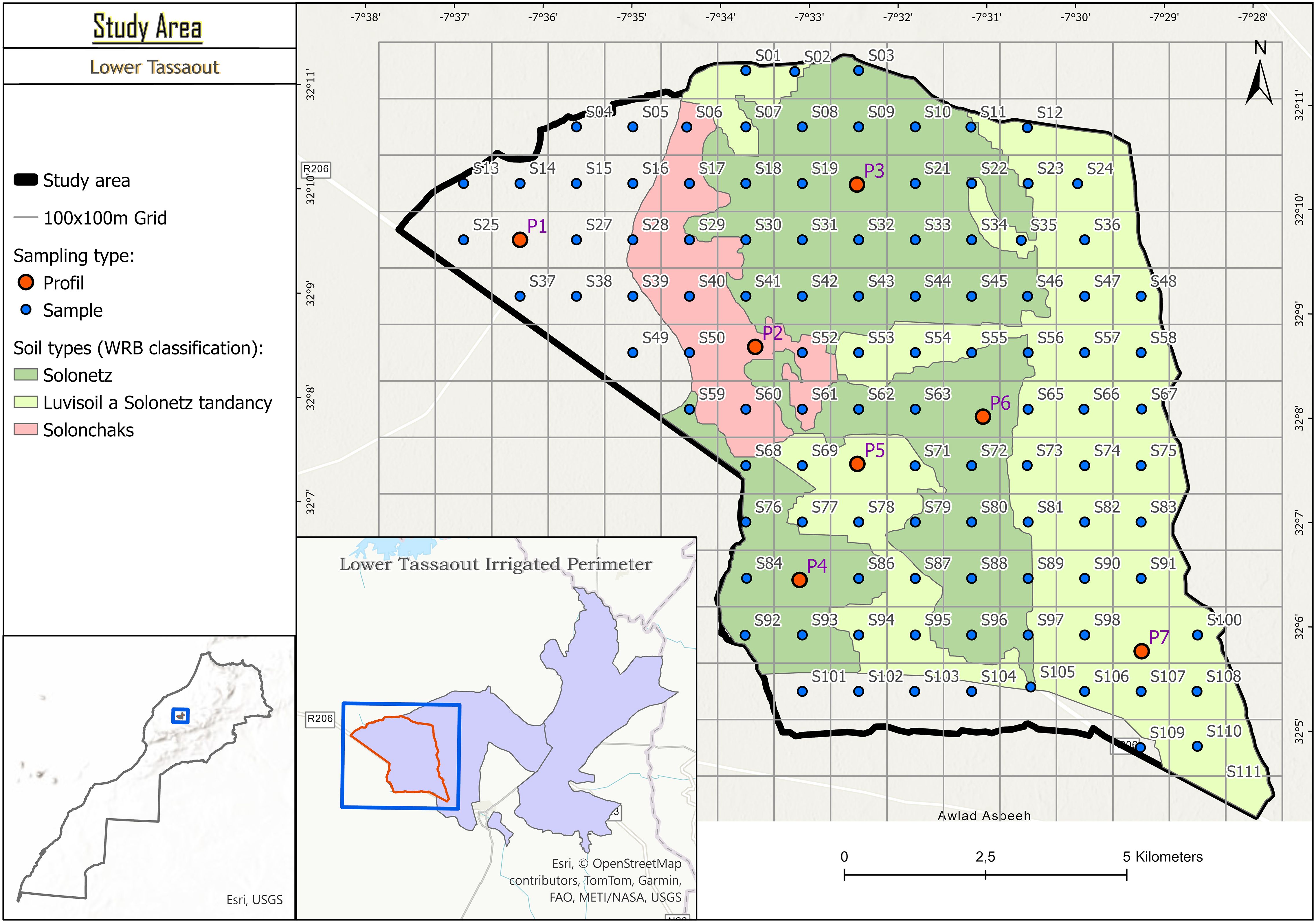
Figure 1. Map showing sampling points in the Tassaout irrigation field of Central Morocco.

According to the World Reference Base (WRB) classification (19), the dominant soil types include Solonetz, Luvisoils with Solonetz tendency, and Solonchaks. The area is predominantly used for irrigated farming, producing cereals (e.g., wheat and barley), vegetables (e.g., tomatoes, onions, and peppers), and fruit crops (e.g., citrus fruits, olives, and melons). Forage crops like alfalfa are also widely cultivated to support livestock. Water for irrigation is primarily sourced from groundwater, with supplemental inputs from seasonal floods and small-scale reservoirs or ponds constructed for water harvesting (20).

2.2 Field sampling design and soil sampling procedure

A representative section of the Lower Tassaout irrigated perimeter was selected as the study area based on preliminary field surveys, historical land use assessments, and consultations with local farmers and agricultural extension agents. The selected zone was chosen for its diversity in soil types and salinity levels, making it suitable for evaluating spatial variability in salinity conditions.

To effectively capture this variability, a 100 m × 100 m grid was superimposed over a 1 km² area, resulting in 103 sampling locations (S01–S111). A stratified random sampling approach was employed, considering both soil type distribution and known salinity gradients to ensure balanced spatial coverage and representative sampling across soil and salinity classes.

At each grid cell, a composite surface soil sample (0 – 20 cm depth) was collected for physico-chemical analysis, including EC_S:W and EC_e. Additionally, seven soil profile pits (P1–P7) were excavated across different zones to assess vertical salinity variation and support the calibration and validation of predictive models. This integrated design provided a comprehensive dataset to evaluate the potential of pXRF spectroscopy as a rapid, non-destructive tool for predicting EC_e in salt-affected soils.

2.3 Soil sample preparation and electrical conductivity measurement

The soil samples were oven-dried at 40 °C to remove excess moisture as described in the ISO 11464 (21) protocol. The dried soil is then ground using a mortar and pestle and sieved through 2-mm mesh to exclude large particles and debris and to maintain the uniformity of samples. For the saturated paste extracts used for EC_e measurement, 200 g of soil was weighed into a 500 ml ceramic dish and mixed with deionized water until a saturated paste was formed, following the method described by Rhoades (22). The paste was carefully observed for the development of a glistening characteristic when light was reflected on it and checked for flowability when the container was tipped. The pastes were allowed to stand overnight until they reached equilibrium. Once prepared, the pastes were placed in mechanical extractors with filter papers on top and syringes attached to connection tubes. The extractor was set to run for one hour to extract the soil paste extracts. Finally, EC_e was measured using a calibrated EC meter (SevenDirect SD30 – Mettler Toledo). In accordance with ISO 11265 (1999) protocol, three soil-to-water suspensions were prepared by weighing 10 grams of soil in 50 ml polypropylene tubes and adding 10, 25, and 50 ml of water, respectively. The tubes were then tightly sealed and shaken at 20 °C for 30 minutes at a speed of 180 rpm while ensuring the soil samples are mixed well with water. Subsequently, the tubes were immediately centrifuged at 3500 rpm for three minutes until supernatant liquid was separated from the soil particles. Finally, EC_S:W measurements were performed in duplicate using the same EC meter used for EC_e determination.

2.4 Soil sample preparation and pXRF measurement

Soil samples for analysis using the pXRF technique in the laboratory were prepared by grinding and sieving through a 180-µm nylon mesh sieve, while the pXRF technique itself remains non-destructive to the sample. The device used for soil measurement was a Tracer 5I (Bruker) portable X-ray fluorescence instrument, which was set to operate at a voltage of 10 keV and a current of 70 µA to excite the elements of interest. Besides, an 8 mm collimator used for providing a focused beam for accurate reading, and to minimize background radiation interference and enhance target element recognition, a blank manual filter was employed. Furthermore, the calibration of the instrument was verified using a conventional metal coupon device. In preparation for measurement, a Soil Light option was chosen in the menu of the device because the Soil Light option is specifically designed for measuring light elements such as calcium (Ca), sodium (Na), magnesium (Mg), and chlorine (Cl), which are key elements for soil salinity and sodicity characterization. Subsequently, measurement of elements was conducted. Each measurement was conducted over a 90-second period to ensure sufficient counting statistics and reliable results are achieved. Figure 2 depicts the workflow of soil measurement using a pXRF technique.

Figure 2

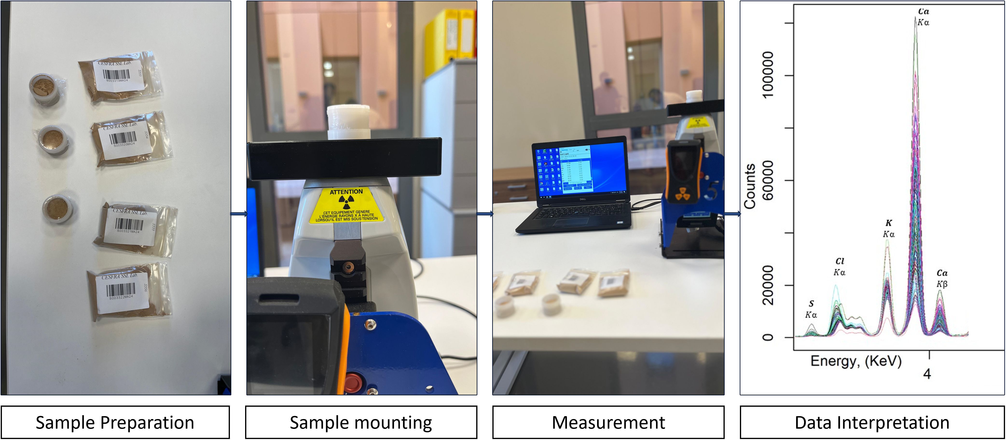
Figure 2. Workflow of pXRF application for the measurement of soil.

2.5 Predictive modeling of soil salinity from pXRF spectra

To evaluate the potential of pXRF spectroscopy for predicting soil salinity, especially EC_S:W and EC_e, two multivariate statistical approaches were employed: principal component analysis (PCA) (23) and partial least squares regression (PLSR) (14). These were applied to explore patterns in the spectral data and to develop predictive models based on elemental signatures related to salinity (24, 25).

PCA was conducted using the “stats” package in R version 4.5.0 (26) and served as an exploratory step to reduce the dimensionality of the pXRF dataset while retaining most of the spectral variability. It transforms correlated spectral variables into uncorrelated principal components (PCs), enabling the identification of sample groupings, outliers, and spectral variance patterns (27). These components also help interpret underlying geochemical gradients related to salinity.

Following PCA, PLSR was used to model the quantitative relationship between the full pXRF spectra (predictor matrix) and the measured EC values (response variables). PLSR is especially suited to spectral data due to its ability to handle high-dimensional and collinear predictors. It projects both predictors and responses onto a new set of latent variables that maximize their covariance, effectively capturing the underlying structure in complex datasets (25).

To avoid overfitting and optimize model performance, the number of latent variables was selected using k-fold cross-validation, with model selection guided by the minimization of the Root Mean Square Error of Cross-Validation (RMSE_CV) and the maximization of R². Once optimized, final models were trained on 75% of the dataset and evaluated on a 25% independent validation set.

Model performance was assessed using three key metrics:

● R² (Coefficient of Determination) Equation 1, representing the proportion of variance explained.

● RMSE (Root Mean Square Error) Equation 2, quantifying prediction error in dS.m^-1.

● RPIQ (Ratio of Performance to Interquartile Range) Equation 3, evaluating model precision relative to natural variability.

$\begin{array}{ll}{R}^2=1-\frac{{\displaystyle \sum {(y_i-{\widehat{y}}_i)}^2}}{{\displaystyle \sum {(y_i-{\overline{y}}_i)}^2}}& (1)\end{array}$

$\begin{array}{ll}RMSE=\sqrt{\frac{{\displaystyle \sum {(y_i-{\widehat{y}}_i)}^2}}{n}}& (2)\end{array}$

$\begin{array}{ll}RPIQ=\frac{IQR(y)}{RMSE}& (3)\end{array}$

where y_i are the observed values, ${\widehat{y}}_i$ are the predicted values, ${\overline{y}}_i$ are the mean of the observed values, n is the number of observations, IQR(y) is the interquartile range 25% - 75% of the observed values. Models with higher R² and RPIQ values and lower RMSE were considered superior in predictive accuracy and robustness.

Additionally, other statistical tests were performed to assess the assumptions and robustness of the models. The Shapiro-Wilk test was conducted to evaluate the normality of residuals, ensuring that the assumptions of linear regression were met. Levene’s Test was used to check for the homogeneity of residuals, confirming that the variance of residuals was consistent across different groups. The Kruskal-Wallis test was applied to test for significant differences between multiple EC groups, particularly when assumptions of normality were violated. Finally, Dunn’s test was used for post-hoc comparisons between EC groups to identify specific differences between them. Together, this modeling and validation framework ensured a comprehensive assessment of predictive performance, addressing not only predictive accuracy but also model robustness, residual behavior, and statistical integrity.

3 Results and discussion

3.1 Effect of soil-to-water ratios on soil EC

Table 1 shows the summary statistics for the soil EC_S:W. For the 1:1 soil-to-water ratio, the electrical conductivities ranged from 0.33 to 77.88 dS.m^-1, while for 1:2.5 and 1:5 ratios, values ranged from 0.17 to 38.87 dS.m^-1 and from 0.09 to 20.96 dS.m^-1, respectively. As expected, EC values decreased progressively with higher dilution ratios due to the reduction in ion concentration. The average EC dropped from 10.85 dS.m^-1 at 1:1 to 2.67 dS.m^-1 at 1:5, confirming this trend.

Table 1

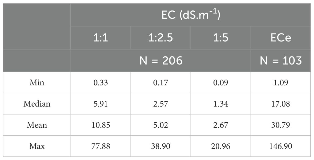
Table 1. Soil EC summary used for establishing EC_1:1, EC_1:2.5, and EC_1:5 relationships.

The equations generated from the linear regressions, shown in Figure 3, demonstrate strong linear correlations between the various dilution ratios with high R² values (all above 0.99). This trend, based on EC values, aligns with findings from Klaustermeier et al. (28), who reported an R² value of 0.91 for the relation between EC_1:1 and EC_1:5. The regression equations indicate a predicted decrease in EC with higher dilution ratios, as evidenced by decreasing slopes corresponding to increasing dilution. The minimal intercepts, approaching zero, suggest that the linear models possess negligible bias, enhancing the reliability of EC predictions across varying ratios. This capability facilitates the estimation of EC at multiple soil-to-water ratios from a single measurement, which is particularly advantageous for rapid or approximate salinity assessments where time or resources are limited. Overall, these findings demonstrate the effectiveness of linear regression models in accurately capturing the relationship between EC values across different dilution ratios.

Figure 3

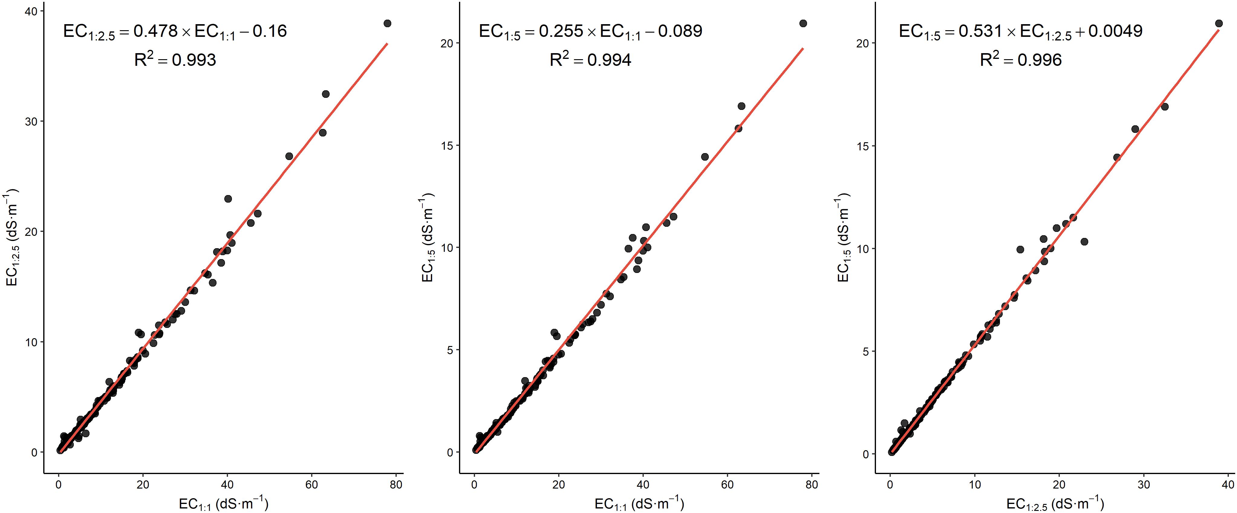
Figure 3. Relationship between different EC_S:W (1:1, 1:2.5, and 1:5).

3.2 Modelling of saturated paste electrical conductivity (EC_e)

The plots in this study (Figure 4) reveal a strong linear relationship between EC_S:W (1:1, 1:2.5, and 1:5) and EC_e, with high R² values of 0.963, 0.944, and 0.950, respectively, confirming that EC_S:W is a reliable predictor of EC_e. As the dilution ratio increases, the regression slope becomes steeper, indicating that EC readings decrease more relative to EC_e, thus requiring larger scaling factors for accurate conversion. This trend reflects the dilution effect, where increased water reduces ion concentration, amplifying the difference between EC_S:W and EC_e. The presence of positive intercepts in each regression suggests a baseline conductivity in the saturated paste that is not influenced by dilution. These results highlight the importance of selecting the appropriate regression equation for each ratio; while the 1:1 ratio shows a more direct relationship, higher ratios like 1:5 require greater adjustment for accurate EC_e estimation.

Figure 4

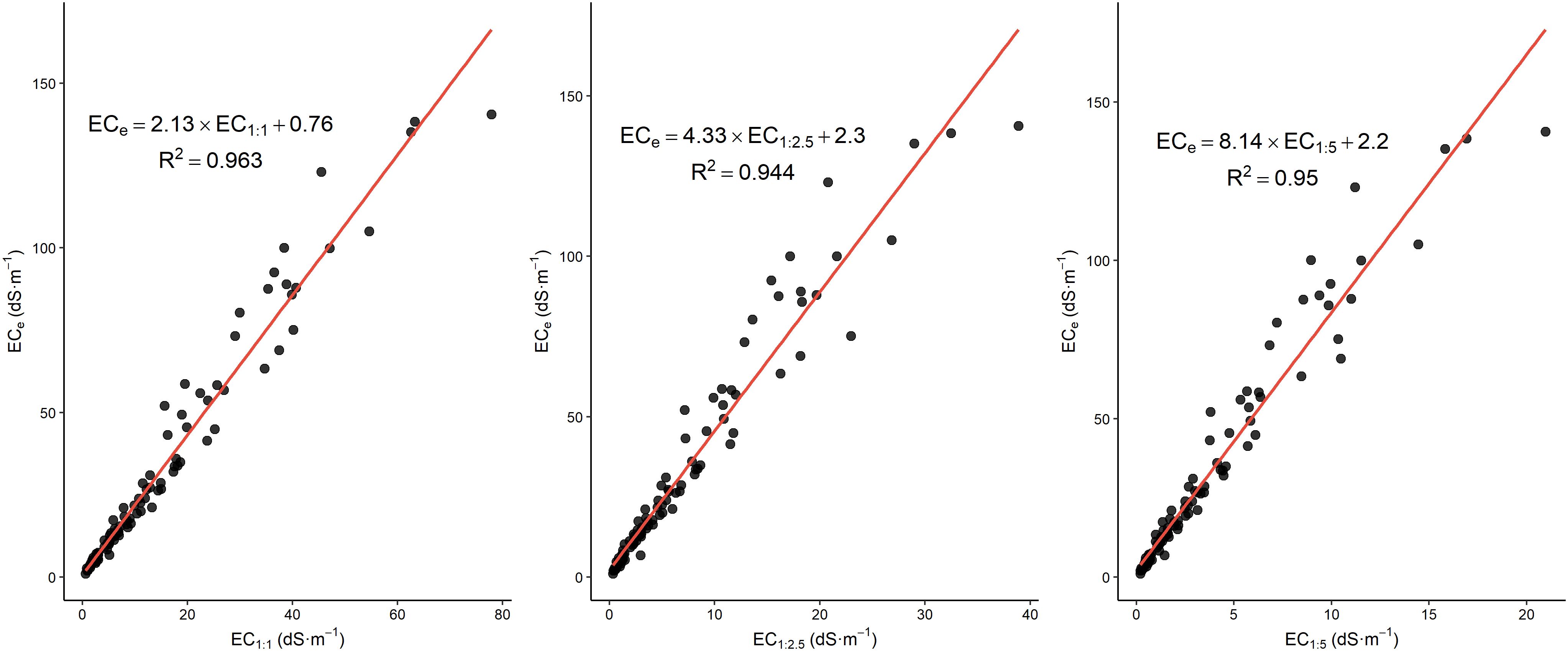
Figure 4. Relationship between EC_e and EC_1:1, EC_1:2.5, and EC_1:5.

Table 2 presents findings from other studies, and our regression models show alignment with these previous results, though with some variations in slopes and interceptions due to methodological differences. For the 1:1 ratio, our regression model EC_e=2.13*EC_1:1 + 0.76 with R² = 0.96 is comparable to previous studies, such as Sonmez et al. (33) with a similar slope of 2.03 and an intercept of -0.41, as well as Zhang et al. (31), who reported EC_e=1.79*EC_1:1 + 1.46. However, our slope is higher than those reported by (30) and (34), which found slopes of 1.56 and 1.83, respectively, indicating stronger EC_e sensitivity in our dataset. This variability could stem from differences in extraction methods and soil compositions across studies.

Table 2

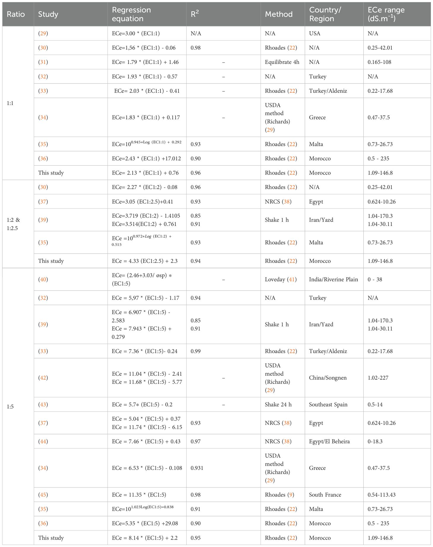
Table 2. Summary of reported ECe correlations with EC_S:W from previous studies.

For the 1:2.5 ratio, our model EC_e=4.33*EC_1:2.5 + 2.3 with R²=0.94 aligns well with (39) for similar ratios, who reported slopes of 3.719 and 3.514 for the 1:2 ratio with R² values of 0.85 and 0.91. The slightly higher slope in our model indicates an increased sensitivity of EC_e to EC_S:W in this ratio, possibly due to the Rhoades method used, which is known to produce precise results for soil salinity.

For the 1:5 ratio, our regression EC_e=8.14*EC_1:5 + 2.2 with R²=0.95 is within the range of slopes reported by previous studies. For example, Sonmez et al. (33) reported a slope of 7.36 with an exceptionally high R² of 0.99, while other studies such as Ozcan et al. (46) and Aboukila et al. (44) reported slopes around 5.97 and 7.46, respectively. Our slope is relatively high compared to these, indicating that EC_e is more sensitive to changes in EC for the 1:5 ratio in our dataset. This increased sensitivity aligns with findings from Marien et al. (45), who observed a slope of 11.35, emphasizing the potential for variability due to differences in soil type, extraction methods, and EC range.

Overall, our study’s results show that EC_e can be accurately estimated from EC_S:W, with differences in slopes and intercepts reflecting methodological diversity across studies. These findings reinforce the importance of using context-specific calibration equations for accurate soil salinity assessments.

3.3 Evaluating pXRF as a diagnostic tool for soil salinity assessment

Figure 5 presents the pXRF spectra of representative soil samples, showcasing the elemental composition through distinct fluorescence peaks. Key elements detected include magnesium (Mg), aluminum (Al), silicon (Si), sulfur (S), chlorine (Cl), potassium (K), calcium (Ca), manganese (Mn), and iron (Fe), corresponding to their characteristic Kα₁ X-ray energies at approximately 1.48 keV, 1.74 keV, 2.31 keV, 2.62 keV, 3.31 keV, 3.69 keV, 5.90 keV, and 6.40 keV, respectively. Among these, Ca exhibits the highest peak intensity at around 4 keV, indicating its substantial presence in the samples. This strong signal is consistent with the role of Ca in maintaining soil structure and influencing salinity, as calcium salts such as CaCl₂ and CaSO₄ are commonly found in arid and semi-arid soils. The prevalence of Ca in these soils also reflects its involvement in cation exchange processes and aggregation stability, both of which are crucial under saline conditions.

Figure 5

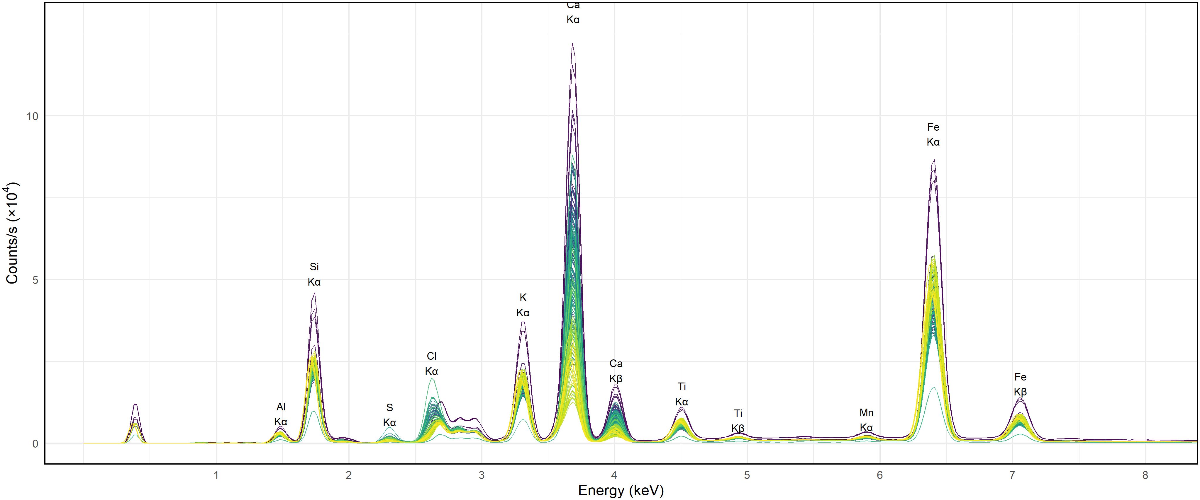
Figure 5. Analysis of pXRF spectra for various soil samples.

Although sodium (Na) is a key driver of soil salinization and sodicity, it was not detected in the pXRF spectra. This is due to the instrument physical limitation: Na emits very low-energy X-rays (~1.04 keV) that are strongly absorbed by air and the detector window, making it difficult for handheld pXRF devices to quantify Na reliably. Consequently, Na was excluded from the measurements. This limitation is well documented in pXRF applications (47), and highlights the need to complement pXRF analysis with conventional laboratory methods when Na quantification is required.

Fe peak near 6.4 keV is also prominent, suggesting a considerable iron content across the samples. While Fe is not directly linked to salinity, its presence influences clay mineralogy and soil fertility, potentially affecting the soil capacity to retain or mobilize salinity-related ions. This is particularly relevant in soils where Fe oxides or Fe-rich clays interact with other salts or affect redox-sensitive elements.

Of particular interest are the peaks of Cl at ~2.6 keV and S at ~2.3 keV, both of which are well-recognized markers of salinity-inducing ions. The high Cl signal suggests accumulation of halite (NaCl) or other chloride-based salts, which are known to significantly elevate soil EC (48). Similarly, the presence of S, often linked with sulfate salts such as gypsum (CaSO₄·2H₂O), further reinforces the connection between the pXRF spectra and salt composition. In agreement with prior studies, both Cl and S show positive correlations with EC (24), reflecting the enrichment of Cl⁻ and SO₄²⁻ ions in the soil and their role in determining salinity status.

The lower intensities of Si and Al further suggest the presence of aluminosilicate minerals, such as quartz and feldspars, which are common in soil matrices and contribute to the structural framework. However, these elements play a minimal direct role in determining salinity when compared to more reactive ions like Ca, Cl, and S.

Altogether, the spectra illustrate the complex interplay between elemental composition and soil salinity. While Cl and S peaks directly inform EC estimation, elements like Fe and Ca reflect both salinity influence and mineralogical background, with intensity variations pointing to differences in parent material or salt accumulation across samples. These findings underscore the utility of pXRF as a rapid, non-destructive tool for simultaneously detecting multiple key elements, enabling a better understanding and management of soil salinity across diverse agricultural and environmental settings.

3.4 Predictive models for EC_S:W and EC_e from pXRF readings.

To estimate soil EC_S:W under various extraction ratios and EC_e from pXRF spectra, Partial Least Squares Regression (PLSR) was selected as the modeling approach due to its demonstrated ability to handle high-dimensional and collinear datasets, characteristics typical of spectral data like that produced by pXRF. In addition to its suitability for such data structures, PLSR is widely supported in the literature as a reliable method for soil salinity prediction. For instance, Naimi et al. (49) evaluated PLSR models for EC_S:W prediction in arid Iranian soils using pXRF data, reporting coefficients of determination (R²) ranging from 0.62 to 0.84, depending on the EC measurement method and dataset partitioning. Similarly, Gozukara et al. (14) assessed multiple machines learning algorithms, including Support Vector Regression (SVR), Random Forest (RF), Cubist, k-Nearest Neighbors (KNN), and PLSR on Turkish soils and found that PLSR achieved R² values between 0.34 and 0.86, ranking among the top-performing models. These findings reinforce the strength of PLSR, which, despite its linear structure, has consistently shown competitive predictive accuracy across diverse salinity contexts. While the current study did not include an internal comparison with alternative machine learning algorithms, the strong and repeatable performance of PLSR in previous studies supports its use here as a robust, interpretable, and well-established baseline for estimating EC_S:W and EC_e from pXRF spectra (Table 3).

Table 3

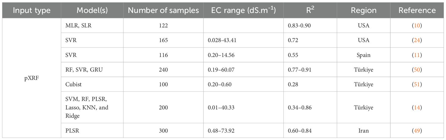
Table 3. Summary of studies predicting EC using pXRF.

Before applying predictive models, principal component analysis (PCA) was conducted to explore the underlying structure and variance within the pXRF spectral dataset. The PCA proportion of variance (Figure 6, left panel) shows that the first two principal components (PC1 and PC2) explain 30.3% and 9.4% of the total variance, respectively, together accounting for nearly 40% of the dataset variability. The sharp decline in explained variance beyond PC2 suggests that the remaining components contribute minimally and are less informative for interpretation. The individual PCA plot (Figure 6, right panel) projects samples onto the PC1 and PC2 plane, where most individuals cluster tightly around the origin, indicating relatively homogeneous variation. However, several samples, such as 1, 2, 3, 5, 12, and 134, appear as outliers, positioned away from the central cluster. These outliers may reflect specific conditions or anomalies, potentially related to variations in soil salinity or differences in EC measurements. The PCA effectively highlights such patterns, supporting the evaluation of pXRF-derived EC estimations (e.g., EC_S:W and EC_e) and revealing meaningful groupings within the data. Overall, the PCA results underscore the utility of this approach in reducing data dimensionality, identifying structure, and guiding further investigation into salinity-related variability among soil samples.

Figure 6

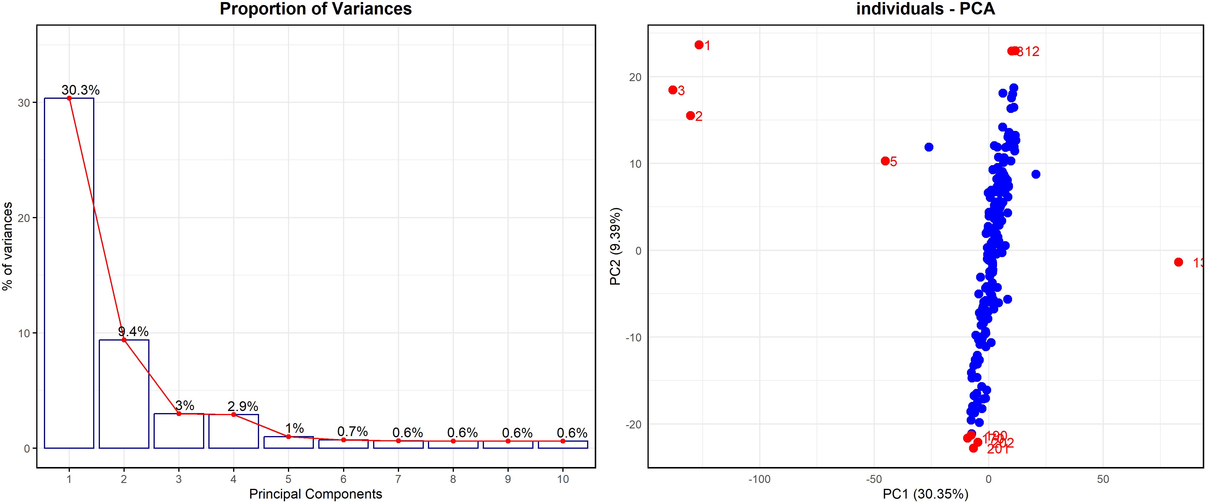
Figure 6. PCA results showing variance and individual clustering.

To gain insight into the spectral features most influential in predicting EC_S:W and EC_e, the loading plot of the first two components (PC1 and PC2) from the PLSR model was examined (Figure 7). These loadings revealed distinct peaks aligned with known elemental emission lines, identifying energy regions most relevant to EC prediction. Positive loadings indicate that higher fluorescence intensity at a given energy is associated with increased EC values, while negative loadings suggest an inverse relationship.

Figure 7

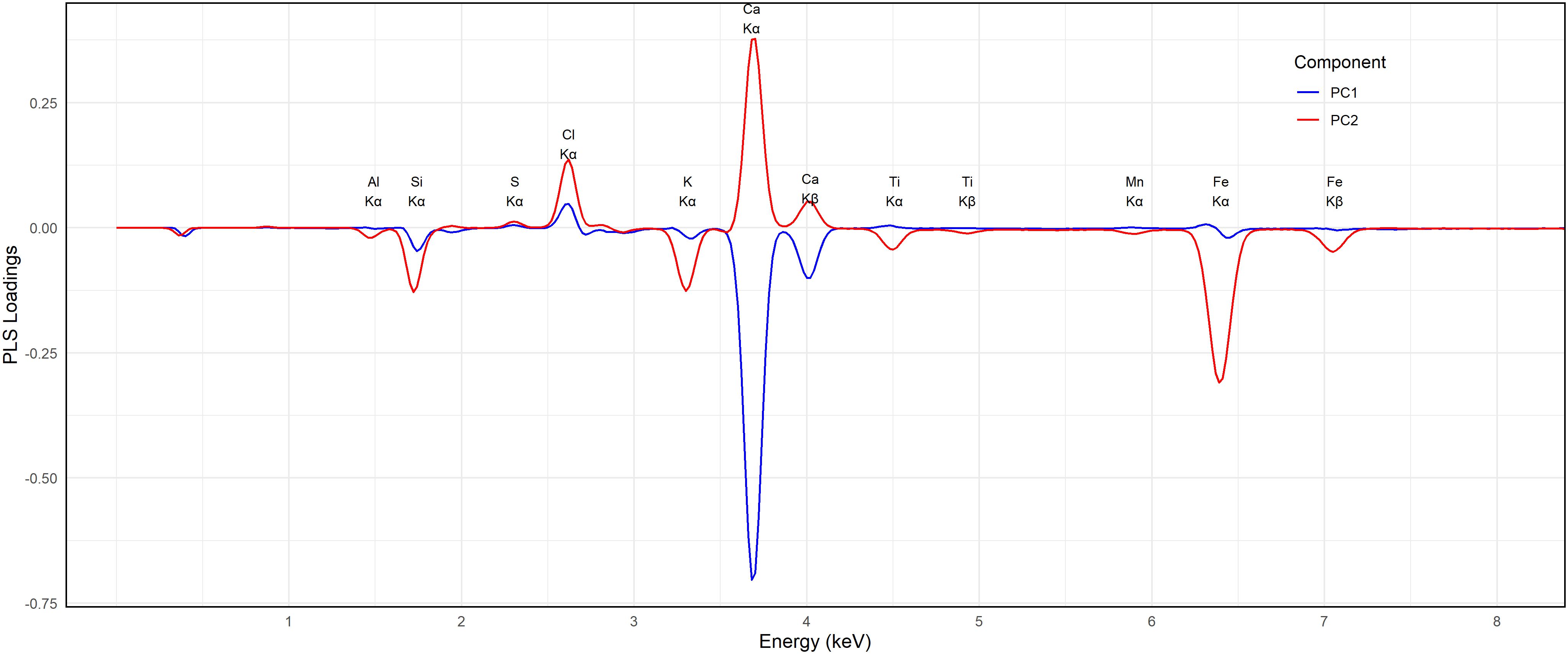
Figure 7. PC1 and PC2 loadings of predicted models.

One of the most prominent features in PC1 was a strong negative loading around 3.7 keV, corresponding to the Kα emission line of calcium (Ca Kα₁ ≈ 3.69 keV) and its associated Kβ line (~4.01 keV). This indicates that higher Ca fluorescence intensities are associated with lower predicted EC values. While calcium salts such as CaCl₂ and CaSO₄ contribute to soil salinity, the inverse relationship may reflect the stabilizing effect of Ca²⁺ on soil structure or its association with non-soluble forms. High calcium content may also reduce the mobility of other salts through buffering or precipitation processes, explaining its negative influence in the model. This region also includes a smaller negative feature at ~3.3 keV, corresponding to potassium (K Kα₁ ≈ 3.31 keV), which partially overlaps with Ca Kβ. Potassium appears to follow a similar trend, though its overall contribution is smaller. Present in both exchangeable forms and clay minerals, K may play a secondary role in EC prediction in this dataset.

In contrast, a strong positive peak was observed in the 6.4 – 7.0 keV range, corresponding to the Kα and Kβ emission lines of iron (Fe Kα₁ ≈ 6.40 keV, Kβ ≈ 7.06 keV). This suggests that higher Fe fluorescence is associated with higher predicted EC values. Although Fe is not a conventional salt-forming ion in soil solution, its correlation with EC may result from its prevalence in clay-rich or alluvial soils that retain more soluble salts. Additionally, in reducing or waterlogged environments, Fe²⁺ can become more mobile, potentially influencing salinity indirectly. Notably, Ca and Fe show opposing signs in the PC1 loadings, suggesting that they capture contrasting geochemical regimes within the dataset.

A moderate positive feature was also observed near 4.5 keV, likely corresponding to titanium (Ti Kα₁ ≈ 4.51 keV). Like Fe, Ti is commonly associated with clay minerals and may reflect underlying mineralogical differences related to salinity. The In summary, the signs and magnitudes of these elemental loadings, particularly the strong negative loading for Ca and the strong positive loading for Fe, highlight their pivotal roles in shaping EC predictions. The model’s high performance (R² ≈ 0.94 – 0.98) supports the interpretation that these elemental fingerprints, especially Ca²⁺ and Fe²⁺/Fe³⁺, are key drivers of salinity- related variability captured by the pXRF-PLSR approach.

3.4.1 Statistical assessment of model performance

The strong predictive performance of all PLSR models (Figure 8), demonstrated by high R² values and low RMSE, is further supported by the RPIQ metric, which offers a normalized assessment of model error relative to the natural variability in EC measurements. PLSR remains one of the most widely applied regression techniques for soil spectroscopy due to its ability to handle collinear spectral data (52).To contextualize model quality, we refer to the classification proposed by Nawar (53), who defined five performance categories based on RPIQ thresholds: models with RPIQ values ≥ 2.5 are considered excellent; those between 2.5 and 2.0 are classified as very good; values between 2.0 and 1.7 indicate a better model; those between 1.7 and 1.4 are deemed reasonable; and values < 1.4 reflect very poor predictive ability. Based on this classification, all models developed in this study fall within the very good to excellent categories, with most validation RPIQ values exceeding 3.0. Specifically, the EC_1:1 model achieved an RPIQ of 3.78, EC_1:2.5 scored 3.43, EC_1:5 reached 3.91, and EC_e produced the highest RPIQ at 4.39. These results confirm the high reliability and robustness of the pXRF–PLSR approach in capturing the relationship between spectral features and salinity-related measurements (54), even when evaluated using an independent validation dataset.

Figure 8

Figure 8. Calibration and validation of PLSR models for predicting soil EC. (A) EC_1:1, (B) EC_1:2.5, (C) EC_1:5, (D) ECe.

In detail, the EC_1:1 model yielded a calibration R² of 0.97, with an RMSE of 1.98 and an RPIQ of 6.04. During validation, the model maintained strong performance with an R² of 0.94, RMSE of 3.23, and RPIQ of 3.78, indicating a good fit with moderate prediction variability on unseen data. The EC_1:2.5 model performed similarly, with a calibration R² of 0.97, RMSE of 1.09, and RPIQ of 4.74, while validation yielded an R² of 0.93, RMSE of 1.55, and RPIQ of 3.43. The slightly higher validation error suggests mild overfitting, though the model remained robust overall.

The EC_1:5 model demonstrated the most consistent performance between calibration and validation. It recorded a calibration R² of 0.95, RMSE of 0.66, and RPIQ of 4.34, while validation achieved an R² of 0.97, RMSE of 0.72, and RPIQ of 3.91. These results reflect strong generalization and stability across different samples. The EC_e model delivered the highest predictive accuracy, with R² values of 0.96 in both calibration and validation. Although its RMSE values were slightly higher, 7.00 and 6.88, respectively, due to the wider range and greater variability of EC_e measurements, it still achieved excellent RPIQ scores of 5.35 and 4.39.

These findings are further supported by a comparison with previously published studies, as summarized in Table 3. For example, Swanhart et al. (10) reported R² values between 0.83 and 0.90 using Multiple Linear Regression (MLR) and Simple Linear Regression (SLR) models, while Aldabaa et al. (24) reported an R² of 0.72 with SVR. Similarly, Weindorf et al. (11) and Gozukara et al. (50) reported R² values of 0.55 and up to 0.91, respectively, using various models and regions. In contrast, the PLSR models in the present study (Table 4) consistently exceeded R² values of 0.93 and achieved lower RMSE, highlighting the added value of using full spectrum pXRF data coupled with optimized multivariate modeling.

Table 4

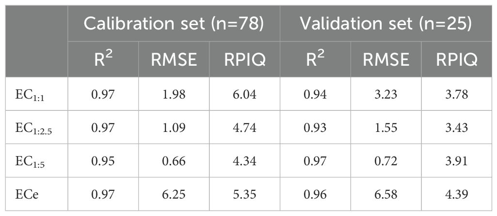
Table 4. Summary of PLSR model calibration and validation for soil EC prediction.

In addition to the performance metrics, model diagnostics were conducted to evaluate residual behavior and assess compliance with statistical assumptions. The Shapiro-Wilk test (Table 5a) revealed that residuals across all EC extraction groups were not normally distributed (p < 2.2 × 10⁻¹⁶), and the Levene test (Table 5b) indicated significant heterogeneity of variance among groups (p < 2.2 × 10⁻¹⁶), violating the assumptions of normality and homoscedasticity. Despite these violations, the Kruskal-Wallis test (Table 5c) showed no statistically significant differences between predicted and observed EC values across models (p > 0.48), and the mean values were nearly identical, differing only at the third decimal place, confirming the absence of systematic bias and strong overall calibration. To further investigate precision differences, Dunn’s post hoc test with Bonferroni correction (Table 5d) was applied. The results showed that the EC_1:5 model had significantly higher residual variability than other models (p < 0.0001), suggesting reduced precision and sensitivity to error under this extraction ratio. In contrast, the EC_e model produced the lowest residuals and significantly outperformed EC_1:1, EC_1:2.5, and EC_1:5, confirming its superior precision despite encompassing a broader salinity range. These findings underscore that while all models provide accurate and unbiased predictions, their precision varies depending on the extraction method. Overall, the results confirm that the pXRF–PLSR framework is a reliable and effective approach for predicting soil salinity across multiple extraction ratios. The EC_1:5 model offers the most stable and consistent performance, making it well-suited for routine and field-based applications, whereas the EC_e model demonstrates the highest predictive power and precision, making it ideal for detailed laboratory-based assessments. The consistently strong RPIQ values across all models further reinforce their ability to deliver accurate and precise predictions relative to the natural variability of EC measurements, supporting the practical use of this method for rapid, non-destructive salinity monitoring in agronomic and environmental contexts.

Table 5

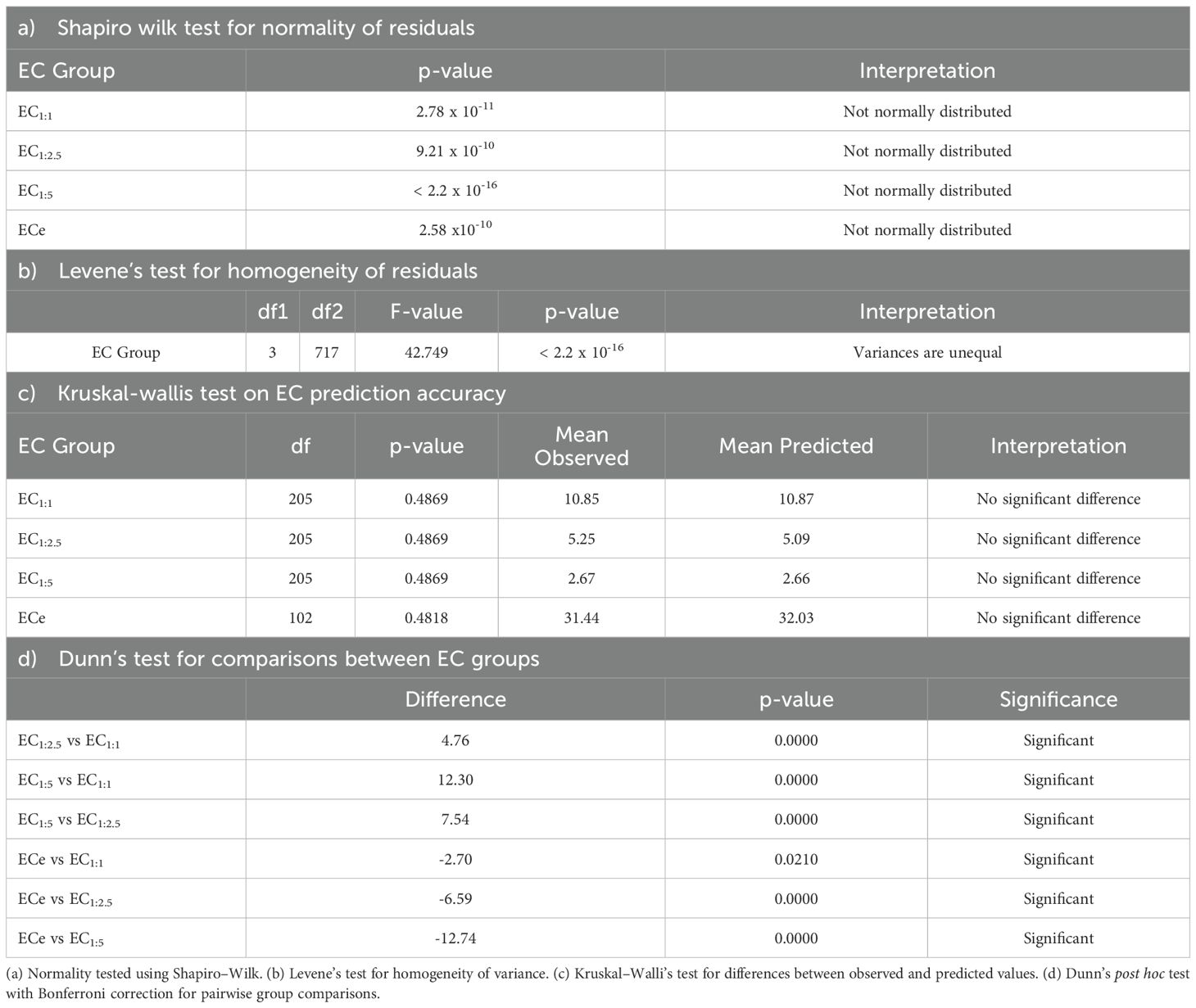
Table 5. Summary of residual diagnostics and group comparisons for PLSR model performance across EC extraction ratios.

4 Conclusion

This study demonstrates the strong potential of pXRF spectroscopy combined with PLSR for predicting soil electrical conductivity, with a particular focus on EC_e. Among the models evaluated, the EC_e model consistently delivered the highest predictive accuracy and precision, with R² values of 0.96 in both calibration and validation, and RPIQ values classified as “excellent” according to established benchmarks. These results confirm that pXRF–PLSR is not only a scientifically robust approach but also a practical tool for rapid, field-relevant assessment of soil salinity.

Unlike conventional laboratory methods that require labor-intensive preparation and delayed analysis, the pXRF-based approach enables in situ, multi-elemental soil analysis in seconds. This dramatically improves the speed and efficiency of salinity monitoring, particularly when applied to large-scale or high-density sampling campaigns. The EC_e model’s strong performance, even under conditions of high intrinsic salinity variability, underscores its suitability for real-world applications especially in irrigated and salt-affected landscapes where EC_e is the most agronomically relevant parameter for assessing soil salinity hazard.

From a land management perspective, pXRF provides a valuable tool for the rapid diagnosis of soil degradation, early detection of salinization, and implementation of timely remediation strategies. Further refinement should focus on improving adaptability to variable field conditions (e.g., moisture content, soil texture) and strengthening calibration across diverse soil types to enhance reliability. Overall, this study confirms that pXRF, coupled with PLSR, offers a scientifically robust and scalable approach for soil salinity assessment, with direct relevance to sustainable land use practices and long-term strategies for salinity control and soil remediation.

Data availability statement

The raw data supporting the conclusions of this article will be made available by the authors, without undue reservation.

Author contributions

TE: Software, Writing – review & editing, Writing – original draft, Formal analysis, Visualization, Validation. AL: Methodology, Writing – review & editing. FK: Resources, Funding acquisition, Writing – review & editing, Supervision, Methodology.

Funding

The author(s) declare that no financial support was received for the research and/or publication of this article.

Acknowledgments

The authors gratefully acknowledge the valuable technical support provided by the CESFRA team at Mohammed VI Polytechnic University (UM6P) throughout the study. Special thanks go to Abdelghani Tikert for his assistance with field data collection, and to Ayoub Lazzar for his technical support. The authors also thank the Soil Spectroscopy Laboratory at CESFRA for its support and collaboration.

Conflict of interest

The authors declare that the research was conducted in the absence of any commercial or financial relationships that could be construed as a potential conflict of interest.

Generative AI statement

The author(s) declare that no Generative AI was used in the creation of this manuscript.

Any alternative text (alt text) provided alongside figures in this article has been generated by Frontiers with the support of artificial intelligence and reasonable efforts have been made to ensure accuracy, including review by the authors wherever possible. If you identify any issues, please contact us.

Publisher’s note

All claims expressed in this article are solely those of the authors and do not necessarily represent those of their affiliated organizations, or those of the publisher, the editors and the reviewers. Any product that may be evaluated in this article, or claim that may be made by its manufacturer, is not guaranteed or endorsed by the publisher.

References

1. El hasini S, Iben. Halima O, El. Azzouzi M, Douaik A, Azim K, and Zouahri A. Organic and inorganic remediation of soils affected by salinity in the Sebkha of Sed El Mesjoune – Marrakech (Morocco). Soil Tillage Res. (2019) 193:153–60. doi: 10.1016/j.still.2019.06.003

Crossref Full Text | Google Scholar

2. Sarath NG, Sruthi P, Shackira AM, and Puthur JT. Halophytes as effective tool for phytodesalination and land reclamation. Front Plant-Soil Interaction: Mol Insights into Plant Adaptation. (2021), 459–94. doi: 10.1016/B978-0-323-90943-3.00020-1

Crossref Full Text | Google Scholar

3. Sharma S, Prasad A, and Prasad M. Osmosensing in plants: mystery unveiled. Trends Plant Sci. (2023) 28:740–2. doi: 10.1016/J.TPLANTS.2023.04.001

PubMed Abstract | Crossref Full Text | Google Scholar

4. Kahime K, Salem AB, El Hidan A, Messouli M, and Chakhchar A. Vulnerability and adaptation strategies to climate change on water resources and agriculture in Morocco: Focus on Marrakech-Tensift-Al Haouz region. Int J Agric Environ Res. (2018) 4(1):58–77. Available online at: www.ijaer.in (Accessed January 11 ,2024).

Google Scholar

5. Debbarh A and Badraoui M. Irrigation et environnement au Maroc: situation actuelle et perpectives. Atelier du PCSI (Programme Commun Systèmes Irrigués) sur une Maîtrise Des Impacts Environnementaux l’Irrigation. (2001), 14.

Google Scholar

6. Rengasamy P. World salinization with emphasis on Australia. J Exp Bot. (2006) 57:1017–23. doi: 10.1093/JXB/ERJ108

PubMed Abstract | Crossref Full Text | Google Scholar

7. Kumar P and Sharma PK. Soil salinity and food security in India. Front Sustain Food Syst. (2020) 4:533781. doi: 10.3389/fsufs.2020.533781

Crossref Full Text | Google Scholar

8. Zhang K, Chang L, Li G, and Li Y. Advances and future research in ecological stoichiometry under saline-alkali stress. Environ Sci pollut Res. (2023) 30:5475–86. doi: 10.1007/s11356-022-24293-x

PubMed Abstract | Crossref Full Text | Google Scholar

9. Rhoades JD, Chanduvi F, and Lesch SM. Soil salinity assessment: Methods and interpretation of electrical conductivity measurements. Food Agric Org. (1999) 57.

Google Scholar

10. Swanhart S, Weindorf DC, Chakraborty S, Bakr N, Zhu Y, Nelson C, et al. Soil salinity measurement via portable X-ray fluorescence spectrometry. Soil Sci. (2014) 179:417–23. doi: 10.1097/SS.0000000000000088

Crossref Full Text | Google Scholar

11. Weindorf DC, Chakraborty S, Herrero J, Li B, Castañeda C, and Choudhury A. Simultaneous assessment of key properties of arid soil by combined PXRF and Vis–NIR data. Eur J Soil Sci. (2016) 67:173–83. doi: 10.1111/EJSS.12320

Crossref Full Text | Google Scholar

12. El Mellouki M, Boularbah A, Agyei Frimpong K, and Kebede F. Portable X-ray fluorescence (pXRF) application for plant nutrition analysis and environmental hazard evaluation in tropical environment. J Plant Nutr. (2025) 48:2295–315. doi: 10.1080/01904167.2025.2476635

Crossref Full Text | Google Scholar

13. Devlin A. Portable X-Ray Fluorescence Spectrometry for Sensing Salinity and Sodicity in Glacial Northern Great Plains Soils with Machine Learning Models. Electronic Theses and Dissertations (2024). Available online at: https://openprairie.sdstate.edu/etd2/969.

Google Scholar

14. Gozukara G, Altunbas S, Dengiz O, and Adak A. Assessing the effect of soil to water ratios and sampling strategies on the prediction of EC and pH using pXRF and Vis-NIR spectra. Comput Electron Agric. (2022) 203:107459. doi: 10.1016/j.compag.2022.107459

Crossref Full Text | Google Scholar

15. Andrade Foronda D and Colinet G. Prediction of soil salinity/sodicity and salt-affected soil classes from soluble salt ions using machine learning algorithms. Soil Syst. (2023) 7:47. doi: 10.3390/SOILSYSTEMS7020047

Crossref Full Text | Google Scholar

16. Wang X, Ainiwaer M, Maimaitituersun A, Zhang J, and Subi X. Prediction of soil salinization in arid regions during wet and dry seasons based on spectro-polarimetric features and machine learning. Land Degrad Dev. (2025) 36:4290–303. doi: 10.1002/ldr.5635

Crossref Full Text | Google Scholar

17. Mirzaee S, Nafchi AM, Ostovari Y, Seifi M, Ghorbani-Dashtaki S, Khodaverdiloo H, et al. Monitoring and assessment of spatiotemporal soil salinization in the Lake Urmia region. Environ Monit Assess. (2024) 196:958. doi: 10.1007/s10661-024-13055-6

PubMed Abstract | Crossref Full Text | Google Scholar

18. Zhu C, Ding J, Zhang Z, Wang J, Chen X, Han L, et al. Soil salinity dynamics in arid oases during irrigated and non-irrigated seasons. Land Degrad Dev. (2023) 34:3823–35. doi: 10.1002/ldr.4632

Crossref Full Text | Google Scholar

19. WRB IWG. World Reference Base for Soil Resources: International soil classification system for naming soils and creating legends for soil maps. 4th ed. Vienna, Austria: International Union of Soil Sciences (IUSS (2022).

Google Scholar

20. El Mostafa EB. Management of irrigation systems in Haouz Region: case study on Upper Tessaout (modern irrigation system) and Talghoumt (traditional irrigation system). (1997).

Google Scholar

21. ISO NF. ISO 11464 (2006) Soil quality : Pretreatment of samples for physico-chemical analysis (2006). Available online at: https://www.iso.org/standard/37718.html (Accessed November 11, 2024). NF X31 - 412/NF ISO 11464 décembre 2006. Ed (01/12/2006).

Google Scholar

22. Rhoades JD. Soluble salts. In: Methods of Soil Analysis: Part 2 Chemical and Microbiological Properties. Agronomy Monograph No. 9, 2nd ed. Madison, WI, USA: American Society of Agronomy and Soil Science Society of America, (1983). p. 167–179.

Google Scholar

23. Allegretta I, Marangoni B, Manzari P, Porfido C, Terzano R, De Pascale O, et al. Macro-classification of meteorites by portable energy dispersive X-ray fluorescence spectroscopy (pED-XRF), principal component analysis (PCA) and machine learning algorithms. Talanta. (2020) 212:120785. doi: 10.1016/j.talanta.2020.120785

PubMed Abstract | Crossref Full Text | Google Scholar

24. Aldabaa AAA, Weindorf DC, Chakraborty S, Sharma A, and Li B. Combination of proximal and remote sensing methods for rapid soil salinity quantification. Geoderma. (2015) 239 – 240:34–46. doi: 10.1016/J.GEODERMA.2014.09.011

Crossref Full Text | Google Scholar

25. Pearson D, Chakraborty S, Duda B, Li B, Weindorf DC, Deb S, et al. Water analysis via portable X-ray fluorescence spectrometry. J Hydrol (Amst). (2017) 544:172–9. doi: 10.1016/J.JHYDROL.2016.11.018

Crossref Full Text | Google Scholar

26. R Core Team. R: A language and environment for statistical computing. Vienna, Austria: R Foundation for Statistical Computing, (2025). Available at: https://www.R-project.org/

Google Scholar

27. Bharadiya JP. A tutorial on principal component analysis for dimensionality reduction in machine learning. Int J Innov Sci Res Technol. (2023) 8:2028–32. doi: 10.5281/zenodo.8002436

Crossref Full Text | Google Scholar

28. Klaustermeier A, Tomlinson H, Daigh ALM, Limb R, DeSutter T, and Sedivec K. Comparison of soil-to-water suspension ratios for determining electrical conductivity of oil-production-water-contaminated soils. Can J Soil Sci. (2016) 96:233–43. doi: 10.1139/cjss-2015-0097

Crossref Full Text | Google Scholar

29. Richards LA. Diagnosis and improvements of saline and alkali soils. Handbook. (1954) 60:129–34. doi: 10.1097/00010694-195408000-00012

Crossref Full Text | Google Scholar

30. Hogg TJ and Henry JL. Comparison of 1: 1 and 1: 2 suspensions and extracts with the saturation extract in estimating salinity in Saskatchewan soils. Can J Soil Sci. (1984) 64:699–704. doi: 10.4141/cjss84-069

Crossref Full Text | Google Scholar

31. Zhang H, Schroder JL, Pittman JJ, Wang JJ, and Payton ME. Soil salinity using saturated paste and 1:1 soil to water extracts. Soil Sci Soc America J. (2005) 69:1146–51. doi: 10.2136/sssaj2004.0267

Crossref Full Text | Google Scholar

32. Ozcan H, Ekinci H, Yigini Y, and Yuksel O. (2006). Comparison of four soil salinity extraction methods, in: Proceedings of 18th International Soil Meeting of” Soil Sustaining Life on Earth, Managing Soil and Technology, Şanlıurfa, Turkey . pp. 697–703.

Google Scholar

33. Sonmez S, Buyuktas D, Okturen F, and Citak S. Assessment of different soil to water ratios (1:1, 1:2.5, 1:5) in soil salinity studies. Geoderma. (2008) 144:361–9. doi: 10.1016/j.geoderma.2007.12.005

Crossref Full Text | Google Scholar

34. Kargas G, Chatzigiakoumis I, Kollias A, Spiliotis D, Massas I, and Kerkides P. Soil salinity assessment using saturated paste and mass soil: water 1:1 and 1:5 ratios extracts. Water (Basel). (2018) 10:1589. doi: 10.3390/w10111589

Crossref Full Text | Google Scholar

35. Spiteri K and Sacco AT. Estimating the electrical conductivity of a saturated soil paste extract ECe from EC1:1, EC 1:2 and EC1:5 soil:water suspension ratios, in calcareous soils from the Mediterranean Islands of Malta. Commun Soil Sci Plant Anal. (2024) 55:1302–12. doi: 10.1080/00103624.2024.2304636

Crossref Full Text | Google Scholar

36. Ouzemou J-E, Laamrani A, El Battay A, and Whalen JK. Predicting soil salinity based on soil/water extracts in a semi-arid Region of Morocco. Soil Syst. (2025) 9:3. doi: 10.3390/soilsystems9010003

Crossref Full Text | Google Scholar

37. Aboukila EF and Norton JB. Estimation of saturated soil paste salinity from soil-water extracts. Soil Sci. (2017) 182:107–13. doi: 10.1097/SS.0000000000000197

Crossref Full Text | Google Scholar

38. NRCS. Method 4.3. 3: Aqueous Extraction. Lincoln, NE: National Soil Survey Center (2011).

Google Scholar

39. Khorsandi F and Yazdi FA. Gypsum and texture effects on the estimation of saturated paste electrical conductivity by two extraction methods. Commun Soil Sci Plant Anal. (2007) 38:1105–17. doi: 10.1080/00103620701278120

Crossref Full Text | Google Scholar

40. Slavich P and Petterson G. Estimating the electrical conductivity of saturated paste extracts from 1:5 soil, water suspensions and texture. Soil Res. (1993) 31:73. doi: 10.1071/SR9930073

Crossref Full Text | Google Scholar

41. Loveday J and Mcintyre D. Methods for analysis of irrigated soils. Soil Sci. (1974) 78:406. doi: 10.1097/00010694-195411000-00021

Crossref Full Text | Google Scholar

42. Chi C-M and Wang Z-C. Characterizing salt-affected soils of songnen plain using saturated paste and 1:5 soil-to-water extraction methods. Arid Land Res Manage. (2010) 24:1–11. doi: 10.1080/15324980903439362

Crossref Full Text | Google Scholar

43. Visconti F, de Paz JM, and Rubio JL. What information does the electrical conductivity of soil water extracts of 1 to 5 ratio (w/v) provide for soil salinity assessment of agricultural irrigated lands? Geoderma. (2010) 154:387–97. doi: 10.1016/j.geoderma.2009.11.012

Crossref Full Text | Google Scholar

44. Aboukila E and Abdelaty E. Assessment of saturated soil paste salinity from 1:2.5 and 1:5 soil-water extracts for coarse textured soils. Alexandria Sci Exchange J. (2017) 38:722–32. doi: 10.21608/asejaiqjsae.2017.4181

Crossref Full Text | Google Scholar

45. Marien L, Crabit A, Dewandel B, Ladouche B, Fleury P, Follain S, et al. Salinity spatial patterns in Mediterranean coastal areas: The legacy of historical water infrastructures. Sci Total Environ. (2023) 899:165730. doi: 10.1016/j.scitotenv.2023.165730

PubMed Abstract | Crossref Full Text | Google Scholar

46. McGarry D. Comparison of four soil water measurement methods. In: Encyclopedia of Soil Science, 2nd ed. Boca Raton, FL, USA: CRC Press, (2005). p. 697–703.

Google Scholar

47. Adams C, Brand C, Dentith M, Fiorentini M, Caruso S, and Mehta M. The use of pXRF for light element geochemical analysis: a review of hardware design limitations and an empirical investigation of air, vacuum, helium flush and detector window technologies. Geochemistry: Exploration Environment Anal. (2020) 20:366–80. doi: 10.1144/geochem2019-076

Crossref Full Text | Google Scholar

48. Zaman M, Shahid SA, and Heng L. Guideline for Salinity Assessment, Mitigation and Adaptation Using Nuclear and Related Techniques. Cham: Springer International Publishing. (2018). doi: 10.1007/978-3-319-96190-3

Crossref Full Text | Google Scholar

49. Naimi S, Ayoubi S, Di Raimo LADL, and Dematte JAM. Quantification of some intrinsic soil properties using proximal sensing in arid lands: Application of Vis-NIR, MIR, and pXRF spectroscopy. Geoderma Regional. (2022) 28:e00484. doi: 10.1016/J.GEODRS.2022.E00484

Crossref Full Text | Google Scholar

50. Gozukara G, Anagun Y, Isik S, Zhang Y, and Hartemink AE. Predicting soil EC using spectroscopy and smartphone-based digital images. Catena (Amst). (2023) 231:107319. doi: 10.1016/j.catena.2023.107319

Crossref Full Text | Google Scholar

51. Gozukara G, Acar M, Ozlu E, Dengiz O, Hartemink AE, and Zhang Y. A soil quality index using Vis-NIR and pXRF spectra of a soil profile. Catena (Amst). (2022) 211:105954. doi: 10.1016/J.CATENA.2021.105954

Crossref Full Text | Google Scholar

52. Barra I, Khiari L, Haefele SM, Sakrabani R, and Kebede F. Optimizing setup of scan number in FTIR spectroscopy using the moment distance index and PLS regression: application to soil spectroscopy. Sci Rep. (2021) 11:13358. doi: 10.1038/s41598-021-92858-w

PubMed Abstract | Crossref Full Text | Google Scholar

53. Nawar S and Mouazen AM. Predictive performance of mobile vis-near infrared spectroscopy for key soil properties at different geographical scales by using spiking and data mining techniques. Catena (Amst). (2017) 151:118–29. doi: 10.1016/j.catena.2016.12.014

Crossref Full Text | Google Scholar

54. Wang Y, Zhao X, and Kowalski BR. X-ray fluorescence calibration with partial least-squares. Appl Spectr. (1990) 44:998–1002. doi: 10.1366/0003702904086867

Crossref Full Text | Google Scholar