Ensemble machine learning for digital mapping of soil pH and electrical conductivity in the Andean agroecosystem of Peru

In agricultural systems, soil pH and electrical conductivity (EC) are crucial chemical properties that directly affect nutrient availability and microbial activity, but the challenging environment of the Peruvian Andes has limited research on their estimation. This study aimed to develop an ensemble learning method to predict soil pH and EC in Andean agroecosystems using environmental predictors. By using simple and weighted averaging, we developed a heterogeneous ensemble learning approach that integrates machine learning (ML) algorithms, including Support Vector Machine (SVM), Artificial Neural Network (ANN), Random Forest (RF), and Extreme Gradient Boosting (XGBoost). The weighted ensemble assigns weights to models based on their predictive accuracy, measured by R² from spatial cross-validation. Spatial patterns are noticeable, and pH displays greater spatial clustering than EC. Elevation was the most important predictor in ML models for both parameters. Ensemble models significantly outperformed individual models, with the weighted ensemble achieving R² >0.93 and reducing RMSE by approximately 72%. Among standalone models, RF and XGBoost performed best for pH, while SVM performed the best for EC. ANN models were the least effective. Uncertainty analysis indicated high confidence in pH predictions but moderate to high uncertainty in EC predictions, suggesting that EC is more challenging to predict. Ensemble models with optimized weighting provide robust and accurate mapping of spatially autocorrelated soil properties. The high-confidence pH maps are reliable for soil management decisions, while EC predictions, though more uncertain, effectively identify priority areas for future sampling and investigation.

1 Introduction

Soil pH and electrical conductivity (EC) are fundamental physicochemical properties that exert a significant influence over agri-environmental systems. Soil pH, a measure of acidity or alkalinity, governs the solubility and bioavailability of essential nutrients and heavy metals, thereby shaping plant growth, microbial activity, and nutrient cycling (1–3)https://www.zotero.org/google-docs/?FyBhZ0. Salt-affected soils pose a significant threat to soil quality and agricultural productivity, particularly in arid and semi-arid regions, as they affect crop yields and soil health, thereby directly impacting food security (4, 5). EC serves as an indicator of soluble salt concentration and is widely used as a proxy for assessing soil salinity levels, with EC measurements being crucial for understanding soil-water-plant relationships (6, 7). Both properties are crucial for assessing soil fertility, crop suitability, and land degradation, particularly in the context of precision agriculture and sustainable land management.

The spatial variability of soil pH and EC is shaped by a complex interplay of factors, including parent material, land use, topography, climate, and human intervention (8, 9) https://www.zotero.org/google-docs/?wq6crv. Accurate mapping of their distribution is crucial for informing soil management strategies, optimizing fertilizer application, and mitigating the effects of salinity-related constraints. In recent years, digital soil mapping (DSM) has emerged as a powerful tool for characterizing such spatial heterogeneity, enabling data-driven decision-making at various spatial scales (10–12). This is especially relevant in the context of intensifying climate change and increasing anthropogenic pressures, both of which are altering key biophysical processes and productivity determinants across agricultural landscapes (13–15) https://www.zotero.org/google-docs/?AQDjhA.

Machine learning (ML) algorithms have become integral to DSM due to their ability to model complex, nonlinear relationships between soil properties and environmental covariates (16; van der 17). Algorithms such as Random Forest (RF), Support Vector Machines (SVM), Decision Trees, and Gradient Boosting Machines (i.e., XGBoost) have been extensively validated and shown to outperform traditional geostatistical approaches in many settings (18, 19). For instance, Vandana et al. (20) demonstrated the superior performance of RF in predicting soil pH and EC using 202 surface samples (0–15 cm) and 14 environmental predictors, achieving high model accuracy (pH: RMSE = 0.014, R² = 0.81; EC: RMSE = 0.134, R² = 0.73). In Arctic regions, RF has demonstrated superior performance compared to K-Nearest Neighbor (KNN) and Cubist algorithms for predicting soil properties (21) https://www.zotero.org/google-docs/?0LDDI1. Similarly, Bandak et al. (22) reported that Decision Tree models exhibited optimal performance for EC prediction over a 24,000-hectare area, identifying soil moisture, elevation, and vegetation indices as major predictors.

Recent studies have demonstrated the effectiveness of various ML approaches across different environments. Feature selection methods combined with machine learning have been shown to eliminate redundant features and effectively improve model performance. Notably, recursive feature elimination (RFE) combined with RF achieves the highest prediction accuracy for soil pH mapping (23). CatBoost models have emerged as particularly effective for predicting soil salinity, demonstrating superior performance compared to Random Forest and XGBoost models, with the ability to handle categorical data being a key advantage (24, 25). Additionally, on-the-go sensing using apparent electrical conductivity (EC) has proven to be a useful, efficient, and cost-effective surrogate to represent within-field soil spatial variability (26, 27).

While individual ML models offer strong predictive capabilities, ensemble approaches such as stacking and bagging have shown promise in further improving spatial accuracy and robustness (28, 29). Mishra et al. (30) emphasized the benefit of using median predictions from multiple ML algorithms to account for model uncertainty and enhance spatial precision. Ensemble strategies that integrate base and meta-learners, combined with rigorous validation methods such as nested cross-validation, have consistently ranked Random Forest among the best-performing models for predicting diverse soil properties (31, 32). Padarian et al. (33) further emphasized the capacity of ensemble models to capture complex, nonlinear relationships in the soil environment, a major advantage for DSM applications.

Ensemble learning with stacked generalization combines the results from multiple ML algorithms to develop an integrated mapping output with relatively stable performance, though this approach remains relatively uncommon in DSM (34, 35). Weighted model averaging approaches have demonstrated effectiveness in mountainous forested areas, with quantile regression forests achieving the best prediction performance in most cases. Model averaging outperformed individual models in several instances (36, 37). Recent applications of stacking ensemble models have demonstrated significant improvements in various environmental applications, including soil moisture prediction, water quality assessment, and agricultural yield forecasting (38, 39).

In mountainous regions, where soil formation is influenced by steep altitudinal gradients, diverse microclimates, and varied land use systems, the spatial prediction of soil properties is particularly challenging (40, 41). Mountain soils encounter several difficulties in digital mapping, including high local variability, non-linear relationships between environmental covariates and soil properties, and limited accessibility in complex topographical settings (42, 43). Despite these complexities, machine learning has shown promising results in regional applications. For example, Carbajal et al. (44) employed RF, SVM, XGBoost, and artificial neural networks (ANN) to predict soil organic carbon (SOC) in the Peruvian Andes, identifying pH as a key explanatory variable. Machine learning-based digital mapping in mountainous terrain has demonstrated significant success, with random forest regression models achieving high performance (R² = 0.80, 0.79, 0.72, and 0.84 for clay, sand, silt, and SOC, respectively) when integrating soil-forming factors of the scorpan model (45).

Although research on ML-based DSM is expanding, significant gaps in our understanding persist (46, 47). The pronounced microclimatic variability and topographic heterogeneity of Andean agroecosystems likely contribute to substantial spatial variation in both pH and EC. These conditions present both a methodological challenge and an opportunity to refine predictive modeling approaches for soil properties in mountainous landscapes (48). Studies have applied ML to predict soil properties in Andean regions, with pH and EC commonly identified as crucial factors in these models. However, no specific studies have used ensemble methods to predict the pH and EC in Andean soils. Most existing studies are concentrated on other soil properties and temperate or semi-arid regions, where soil-forming factors and land use pressures differ significantly from high Andean environments (49, 50). As such, the application of ensemble learning strategies for the DSM of soil pH and EC in Andean agroecosystems remains underexplored. Addressing this gap is essential for supporting precision agriculture, guiding soil conservation efforts, and promoting climate-resilient land management in one of the world’s most environmentally and agriculturally diverse regions (51, 52).

This study develops an ensemble method for predicting soil pH and electrical conductivity (EC) in Andean agroecosystems using environmental covariates. The key contributions are: (1) enhanced prediction accuracy through stacking ensemble approaches that integrate Random Forest (RF), Support Vector Machines (SVM), Artificial Neural Networks (ANN), and Extreme Gradient Boosting (XGBoost) algorithms; (2) improved spatial mapping in mountainous terrain with high heterogeneity by combining the complementary strengths of each base learner; and (3) demonstration of ensemble learning potential for digital soil mapping in precision agriculture and sustainable land management of Andean environments.

2 Materials and methods

2.1 Study area

The Alto Mantaro sub-basin (11°30’-12°04’S, 75°05’-75°49’W) encompasses 2,114.82 km² in the northwestern Mantaro River basin (Figure 1). As indicated on the Warren Thornthwaite climate classification map provided by the Peruvian National Meteorology and Hydrology Service (SENAMHI), the most important area is characterized by a semi-dry, temperate, and humid climate throughout the year (53). The data indicates a maximum temperature range of 21-25°C, a minimum range of 7-11°C, and annual precipitation estimates between 700 and 2000 millimeters. Leptosols are the most common soil type, characterized by their shallow depth, stony composition, poor development, and lack of distinct features. Formed on solid rock in mountainous regions, these areas are highly susceptible to erosion and have limited agricultural value, though they are used for extensive grazing (54). According to the Ecological and Economic Zoning of the Junín department, the study area exhibits predominant soil textures of sandy loam (34.87%), loam (12.75%), and clay loam (9.65%). The vegetation is primarily Andean grasslands, which account for over 50% of the total area. Moderately steep hills and mountains (15-25° slopes) constitute 26.70% of the area, and agricultural lands span 672.07 km² (31.77%) across the Mantaro Valley provinces of Jauja, Concepción, and Huancayo (55). The sub-basin encompasses 59 districts and 438 population centers, comprising 356,440 inhabitants and 89,345 dwellings (56).

Figure 1

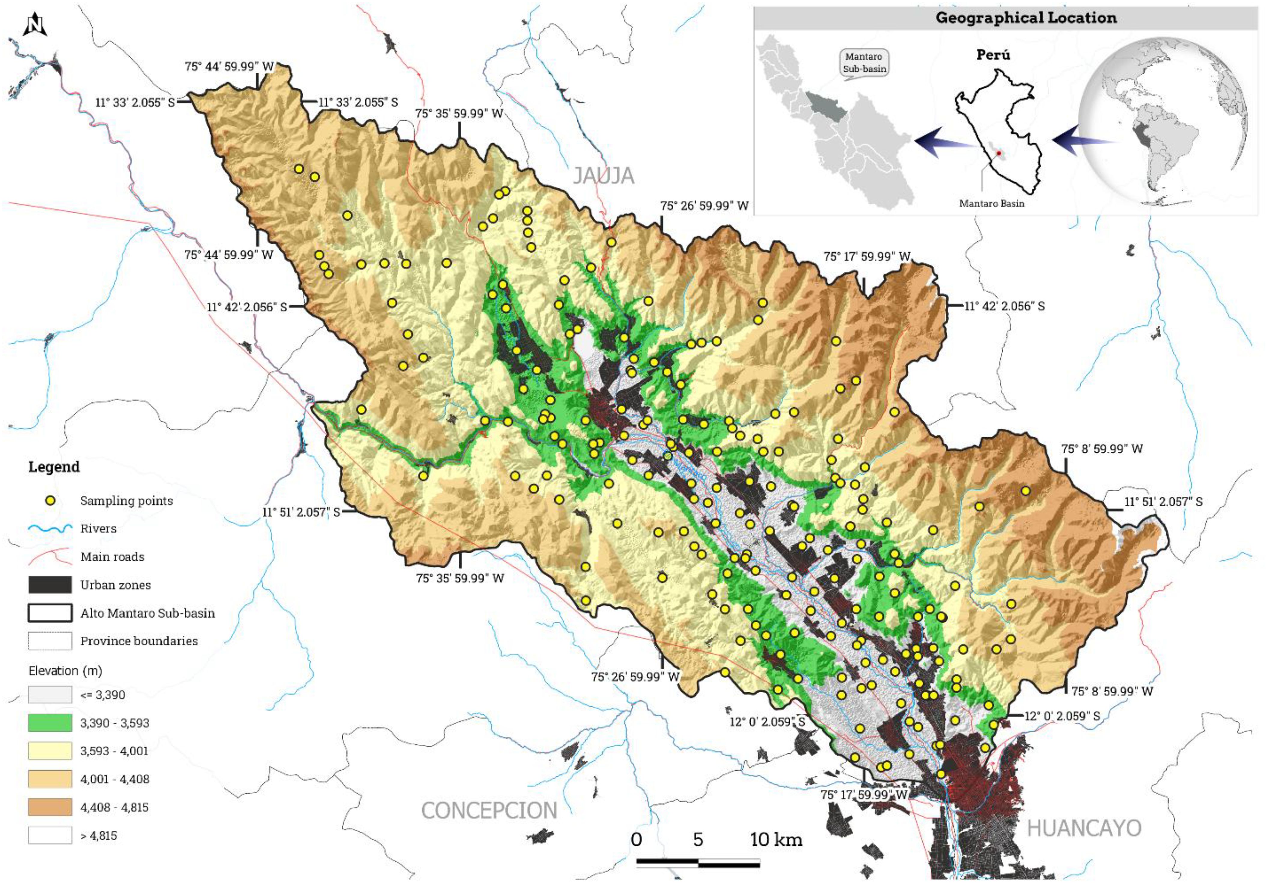
Figure 1. Study area indicating soil sampling locations and elevation features.

2.2 Soil sampling and laboratory analysis

A conditioned Latin hypercube sample (cLHS) was used to determine 204 sample points. Stratified random sampling, based on covariate distributions, is used by the cLHS method to select samples. This improves the sampling scheme by minimizing an energy function that reflects its accuracy in approximating a Latin hypercube for all covariate distributions (57, 58). Spatial sampling points were determined using the clhs R package (59), incorporating elevation, slope, profile curvature, plan curvature, aspect, valley depth, topographic wetness index, topographic position index, land surface temperature, transformed soil-adjusted vegetation index, and accumulated cost as covariates. At each sampling location, samples were collected at a 30 cm depth and later analyzed for pH using the EPA guideline (USEPA 2004), and EC was determined with the saturation extract method (60) at the LABSAF (Soil, Water, and Foliar Laboratory) of the Santa Ana Agrarian Experimental Station.

2.3 Environmental predictors

Soil-forming factors, such as topography and vegetation, along with soil physical and moisture properties, are represented by a set of 21 environmental predictors. Three primary sources of spatial information were employed in this investigation: remote sensing imagery (RS), a digital elevation model (DEM), and soil properties derived from the SoilGrids database (16). Multiple spectral indices (Table 1) were computed from Landsat 8 OLI imagery spanning February through August 2023, which was acquired through the Google Earth Engine (GEE) platform (69). Utilizing SAGA software (70), we generated a suite of topographic predictors from DEM, including aspect, topographic position index (TPI), topographic ruggedness index (TRI), slope, and topographic wetness index (TWI). The study also included properties such as soil texture (clay, sand, silt), bulk density (BD), and volumetric water content (VWC) at three key moisture levels: field capacity (-33 kPa), permanent wilting point (-1500 kPa), and saturation (-10 kPa).

Table 1

Table 1. List of the indices derived from remote sensing used for spatial modeling.

2.4 Exploratory spatial data analysis

2.4.1 Spatial autocorrelation

Spatial autocorrelation measures the extent to which nearby data points in a geographic dataset are related to one another. It essentially assesses the probability of spatially adjacent values being similar. This phenomenon plays a crucial role in interpreting spatial patterns and relationships in data, significantly impacting environmental and geographical research, including soil science. We analyzed spatial autocorrelation in soil EC and pH data using Moran’s I (Equation 1) and Geary’s C (Equation 2) statistics.

$\begin{array}{ll}I=\frac{n}{W}·\frac{{\sum }_i{\sum }_j{w}_{ij}(x_i-\overline{x})(x_j-\overline{x})}{{\sum }_i{(x_i-\overline{x})}^2}& (1)\end{array}$

$\begin{array}{ll}C=\frac{(n-1)}{2W}·\frac{{\sum }_{i=1}^n{\sum }_{j=1}^n{w}_{ij}{(x_i-x_j)}^2}{{\sum }_{i=1}^n{(x_i-\overline{x})}^2}& (2)\end{array}$

Where:

n = number of observations

$$x_i,x_j=\text{observed values at locations }i\text{ and }j.$$

$$\overline{x}=\text{mean of all observations}.$$

$$w_{ij}=\text{spatial weight between locations }i\text{ and }j.$$

$$W=\sum _{i=1}^n\sum _{j=1}^n{w}_{ij}=\text{sum of all spatial weights}.$$

Spatial autocorrelation in geographical data is often measured using Moran’s I and Geary’s C (71, 72). A Moran’s I value close to +1 signifies robust positive spatial autocorrelation, whereas values near -1 denote spatial dispersion. In contrast, Geary’s C demonstrates an inverse association; accordingly, lower Geary’s C values reflect increased clustering within the data. To define spatial neighbors, we utilized the spdep package (73). Graphics such as the Moran scatterplot enable the visualization of the relationship between the value at each location and the values of neighboring locations. This indicates whether the data exhibits positive spatial autocorrelation (where similar values cluster together), negative spatial autocorrelation (where dissimilar values cluster together), or no autocorrelation (indicating a random distribution). We used Local Indicators of Spatial Autocorrelation (LISA) cluster classification to generate a spatial representation with significant clusters: “High-High” (hotspots), “Low-Low” (cold spots), “High-Low” (spatial outliers), and “Low-High” (spatial outliers).

2.4.2 Feature selection

A correlation plot (matrix heatmap) was generated to explore variables and their relationships, with particular focus placed on highly correlated covariates that might not contribute to the modeling. Subsequently, random feature subset search (RFSS) was employed to select model predictors. Sixty subsets were evaluated to determine their respective pH and EC variables. As a fundamental aspect of the Random Forest methodology, RFSS was developed to constrain each ensemble model to a random selection of features, thereby improving performance through a bias-variance trade-off and enhancing diversity. The mlr3 ecosystem was utilized, specifically the mlr3select package (74), with root mean square error (RMSE) employed as the measure of efficiency.

2.5 Machine learning models

Four ML models were used: SVM, ANN, RF, and XGBoost. A variety of regression models, each fine-tuned with specific hyperparameters, were developed for later use in ML tasks like training, validation, and ensembling. To understand why we got a specific result from our predictors (75) and to help interpret the models, we performed Feature Importance Analysis (FIA) only for RF and XGBoost. Importance scores were extracted directly from the trained model and tabulated for convenient plotting.

2.5.1 Support vector machine

The theoretical basis of SVM is based on the work of Vapnik et al. (76), which discusses its use for regression estimation, multidimensional splines construction, and solving linear operator equations, showcasing its versatility in function approximation. In this study, an SVM regression model was implemented using the e1071 R package (77) with a radial basis function (RBF) kernel. During operation, an SVM implicitly transforms data points into an infinitely dimensional space, seeking a linear hyperplane within it. The parameter type was defined as eps-regression, described as standard epsilon-insensitive regression. A tube of width 2*epsilon was created around the regression line by this method, within which errors were disregarded. Hyperparameters such as cost or C were employed, which control the penalty for misclassification of training points. The use of a high C value can result in a smaller margin and overfitting if the data is noisy, as the model aims to accurately classify all training examples. In contrast, a lower C value increases the margin, potentially misclassifying more data points but leading to better generalization. C was set to 10 to achieve a good balance between model complexity and training error. We also used the hyperparameter gamma to adjust the influence of single training examples. Lower values indicate a smoother decision boundary; in this case, we choose a 0.1 value. Lastly, predictions within a ±0.1-unit margin of tolerance were deemed accurate and penalty-free, utilizing an epsilon parameter set to 0.1.

2.5.2 Artificial neural networks

Inspired by biology, the ANN started with the Perceptron, the first trainable neural network (78). It evolved to multilayer networks with backpropagation, leading to practical learning algorithms (79). An ANN regression model was defined using the nnet R package (80). In this case, non-linear patterns were learned using a single-layer feedforward neural network with weighted connections. During model definition, the parameters size, maxit, and decay were taken into account. The size parameter was employed to set the number of units (neurons) in the hidden layer; a size of 10 was selected, which determines the network’s capacity to learn complex patterns. A maxit value of 500 was applied to set the maximum number of iterations. To prevent overfitting, a decay value of 0.01 was implemented for weight decay regularization, which penalizes large weights.

2.5.3 Random forest

The RF emerged from the work of Leo Breiman, building on ensemble methods like bagging, where multiple models are trained on different data samples (81), and incorporating the feature randomness aspect from the random subspace method (82). This model effectively handles missing data, identifies key variables, resists overfitting, and is user-friendly, providing easily interpretable results for diverse data types (83). The prediction function of an RF-like learner was developed with the ranger R package (84). This ensemble method builds decision trees and averages their predictions. Our model incorporated parameters such as the number of trees set to 500 and mtry, which represents the number of randomly selected variables per split and equals the square root of the total number of features. This introduces randomness and reduces overfitting. Other parameters include min.node.size, set to 5, which determines the minimum number of samples in a terminal node, controls tree depth, and prevents overfitting. By quantifying impurity reduction, the importance parameter ranks the covariates, showing which are most crucial for accurate predictions.

2.5.4 Extreme gradient boosting

XGBoost epitomizes the advancements in gradient boosting methodologies. By incorporating novel regularization strategies and computational optimization methods, XGBoost delivers a more resilient and scalable algorithm (85). This model boasts state-of-the-art performance, efficient handling of missing data, built-in regularization, and rapid training (86). The best results usually come from structured or heterogeneous tabular data (87). The XGBoost regression model was implemented using the xgboost R package (88). This gradient boosting method constructs trees sequentially, with each tree designed to correct errors produced by preceding trees. Model complexity is regulated through the critical parameter nrounds, which was configured to 100, thereby specifying the number of boosting rounds (trees). Additional key parameters were employed, including the learning rate (eta), which was established at 0.1. The maximum depth of each tree was configured to be 6, thereby controlling the complexity of individual trees. Randomness was introduced through the subsample parameter, set to 0.7, which prevents overfitting by determining the sample fraction utilized per tree. Similarly, the colsample_bytree parameter was also established at 0.7, providing additional randomization by specifying the fraction of features employed for each tree, thus enhancing model generalization.

2.6 Ensemble approach development

Ensemble Machine Learning is a powerful approach that combines multiple models to improve prediction accuracy and robustness (89), with success in various real-world applications and problem domains (90). The ML ensemble approach was presented using a four-stage flowchart (Figure 2). We implemented two types of ensemble models: a simple average ensemble using bagging-inspired equal weighting across heterogeneous models and a performance-weighted ensemble using stacking-inspired optimization based on spatial cross-validation scores. The first method was based on the arithmetic mean of all four model predictions, following the “wisdom of crowds” philosophy, which assumed that each model contributed equally valuable information. This approach was characterized as simple and robust and effectively minimized individual model bias. The second method was based on a weighted combination derived from spatial cross-validation performance. Greater influence was assigned to models with superior performance through this technique, leveraging their strengths to potentially achieve enhanced overall results. Normalized weights were calculated proportionally using spatial cross-validation R² values, with a minimum weight applied to each model to avoid zero weights (higher R² values were assigned higher weights). The three previously mentioned metrics were also employed to evaluate the performance of both ensemble approaches. A comprehensive table was constructed to compare the performance of ensemble and individual machine learning models.

Figure 2

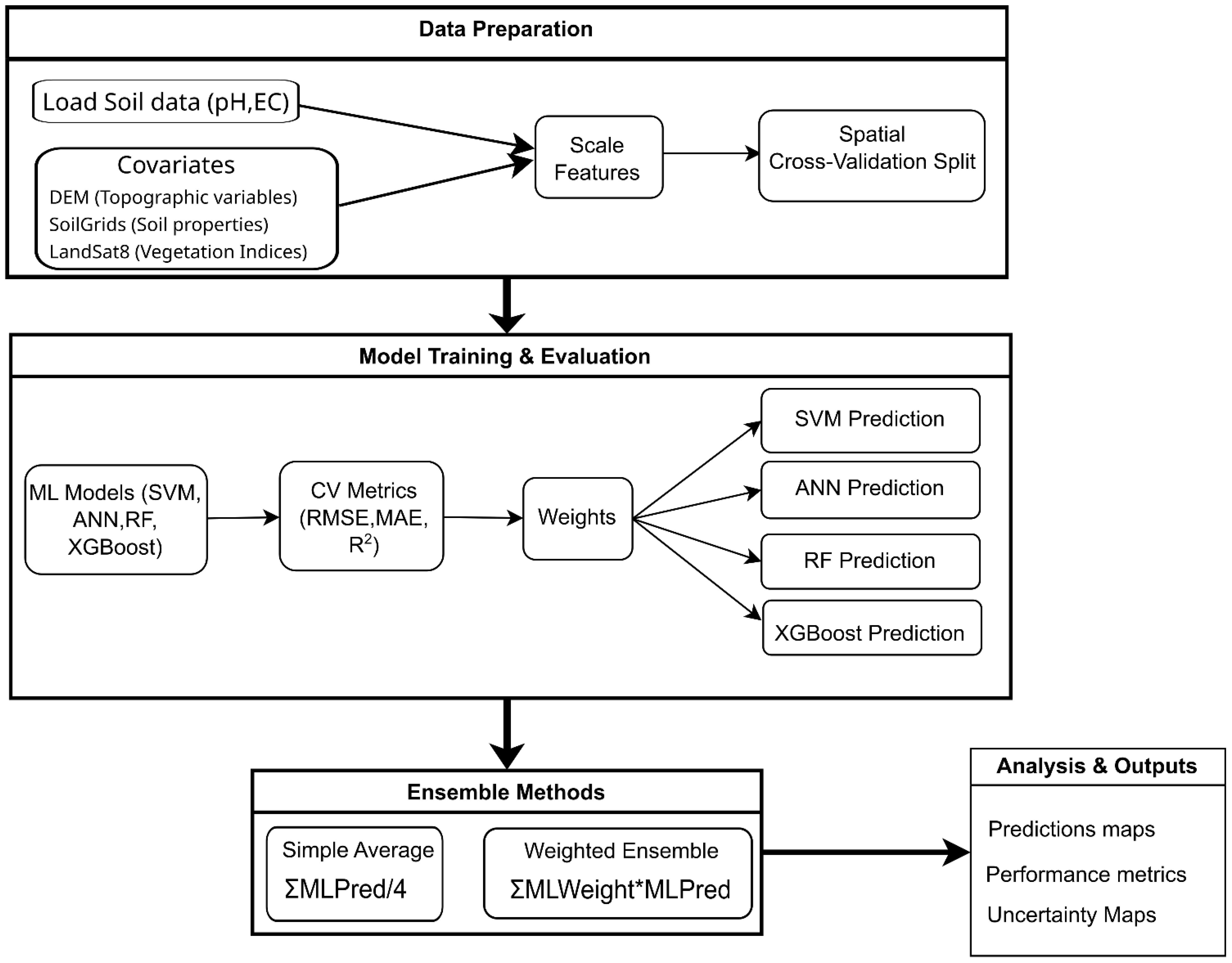
Figure 2. Procedure using the ensemble approach.

2.7 Raster predictions

Raster predictions of pH and EC were generated for the entire study area using trained ML models to create continuous spatial maps. The main methodology, illustrated in the flowchart (Figure 3), involved pixel-by-pixel model application across the study area using the terra package’s predict function. Previously, the input data required preprocessing steps such as scaling, which was crucial for scale-sensitive models like SVM and ANN. Additionally, imputation was necessary to manage missing values (NA pixels); otherwise, a single missing pixel could have rendered the entire prediction invalid. Raster predictions were created for every ML model and both ensemble methods that were evaluated.

Figure 3

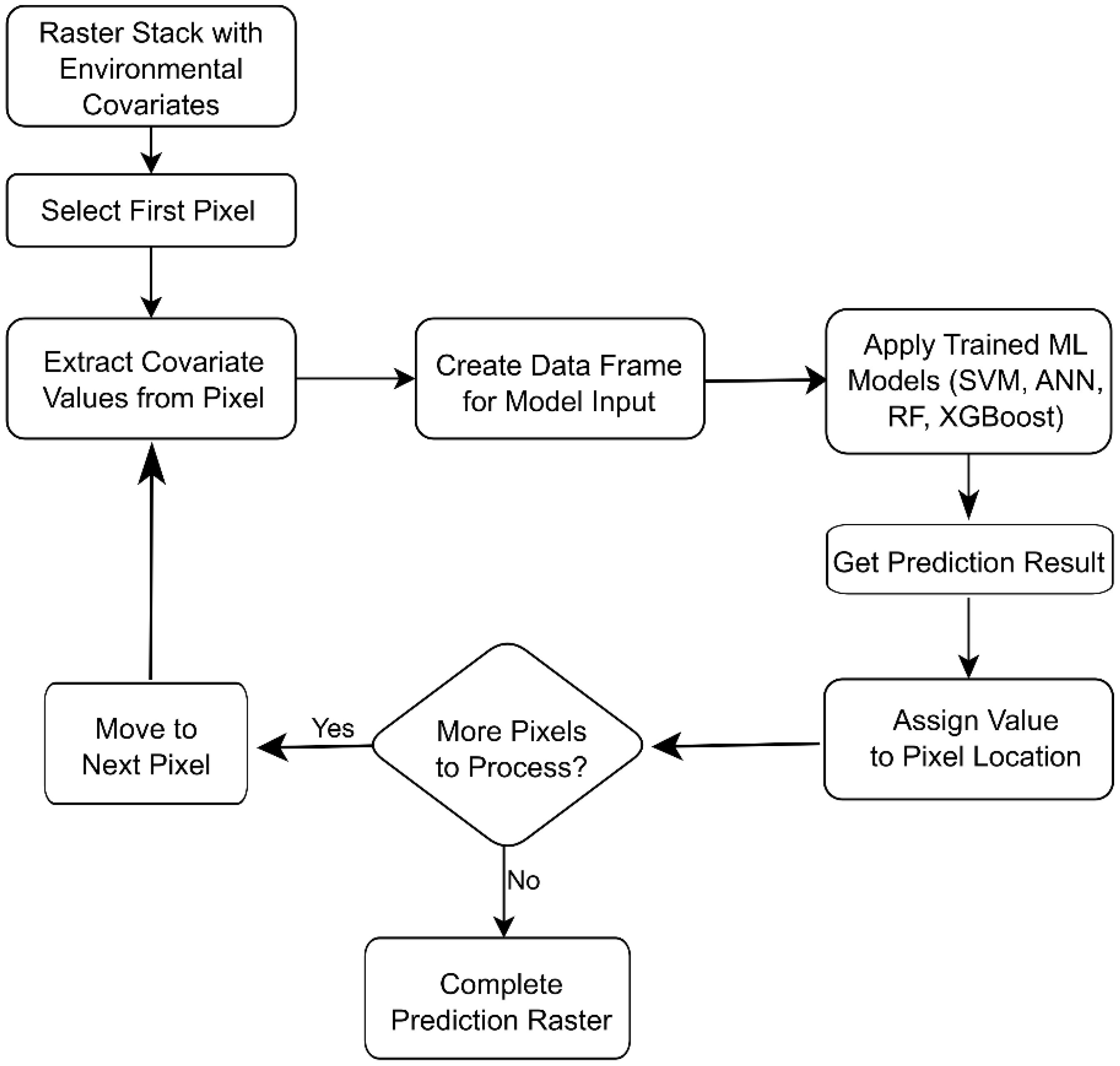
Figure 3. Flowchart to generate raster prediction maps.

2.8 Model calibration and validation

A thorough spatial cross-validation (SP-CV) process was developed to evaluate each ML model. Data splitting was conducted using the spatial block cross-validation method, which divided the study area into five folds using a 3×3 grid. The process proceeded with iterative training for each fold, where models were trained on four spatial blocks (training) and subsequently predicted the remaining spatial block (testing). For evaluation purposes, Root Mean Square Error (RMSE), Mean Absolute Error (MAE), and Coefficient of determination (R²) were calculated for each fold (Equations 3–5), and average performance across all five folds was obtained through the aggregation process. This analysis was conducted to evaluate the performance of ML models, providing realistic assessments of how accurately each model predicted the response variable in unobserved spatial locations. The SP-CV method was considered crucial for accurate soil mapping, as it ensured reliable model predictions in unsampled areas.

$\begin{array}{ll}RMSE=\sqrt{\frac{1}{n}{\displaystyle {\sum }_{i=1}^n{(y_i-\widehat{y_i})}^2}}& (3)\end{array}$

$\begin{array}{ll}MAE=\frac{1}{n}{\displaystyle {\sum }_{i=1}^n\left|y_i-\widehat{y_i}\right|}& (4)\end{array}$

$\begin{array}{ll}{R}^2=1-\frac{{\sum }_{i=1}^n{(y_i-\widehat{y_i})}^2}{{\sum }_{i=1}^n{(y_i-\overline{y})}^2}& (5)\end{array}$

where $y_i$ are the observed values, $\widehat{y_i}$ are the predicted values, $\overline{y}$ the mean of the observed values, and n is the number of samples.

Our evaluation encompassed an uncertainty analysis of the generated raster predictions, employing the coefficient of variation (CV) to quantify the relative variability of predictions from the highest-performing model. Models disagree more and are less certain when CV values are high.

3 Results

3.1 Descriptive statistics of soil properties

Summary statistics for soil properties (response variables), based on 204 data points, are shown in Table 2. Our soils range in pH from strongly acidic to moderately alkaline (pH 4.2 – 8.0), with moderate variability and slightly negative skew. In contrast to EC, there is a broad range of values from 0.9 to 78.8 mS m^-1 (non-saline to moderately saline), with extremely high variability and highly positively skewed. The variations of pH (Figure 4A) and EC (Figure 4B) with elevation are displayed to illustrate a pattern. A trend of increasing pH and EC from higher to lower elevations was observed, with the highest values concentrated in the central valley.

Table 2

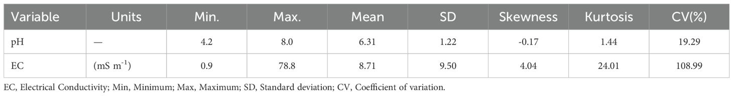
Table 2. Summary of descriptive statistics for predictors and response variables.

Figure 4

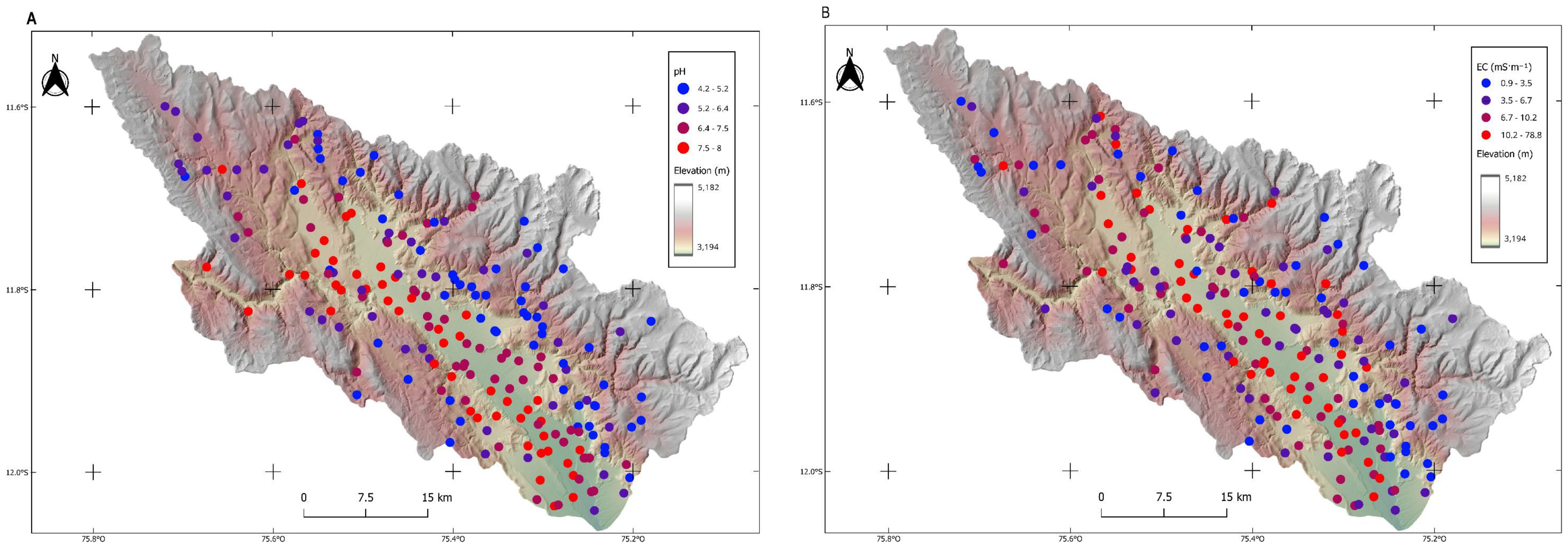
Figure 4. (A) pH value variations in relation to elevation. (B) Electrical conductivity variations in relation to elevation.

3.2 Identification of spatial autocorrelation

The analysis of spatial autocorrelation, using Moran’s I and Geary’s C, found notable positive autocorrelation in the soil properties. The data in Table 3 reveals a high degree of spatial clustering in soil pH (I = 0.500, C = 0.506, p< 0.001), in contrast to EC, which presents only moderate spatial autocorrelation (I = 0.295, C = 0.755, p< 0.001). The stronger spatial structure that was observed in pH compared to EC indicated that pH distribution was more strongly influenced by landscape-level controls, while more localized variation was exhibited by EC. The use of spatial modeling approaches was justified by these results, and spatial cross-validation was necessitated to avoid overoptimistic performance estimates.

Table 3

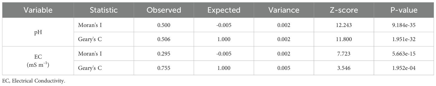
Table 3. Spatial autocorrelation analysis.

A Moran scatterplot was used to visualize the relationship between variables and their spatially lagged neighbors in the autocorrelation analysis. The pH plot displayed a strong positive correlation, with data points clustering densely in the high-high (HH, top-right) and low-low (LL, bottom-left) quadrants, demonstrating pronounced spatial autocorrelation (Figure 5A). In contrast, the EC plot exhibited a similar positive trend but with greater scatter and notable presence of outliers in the high-low (HL, top-left) and low-high (LH, bottom-right) quadrants, indicating moderate positive spatial autocorrelation with more heterogeneous spatial patterns (Figure 5B).

Figure 5

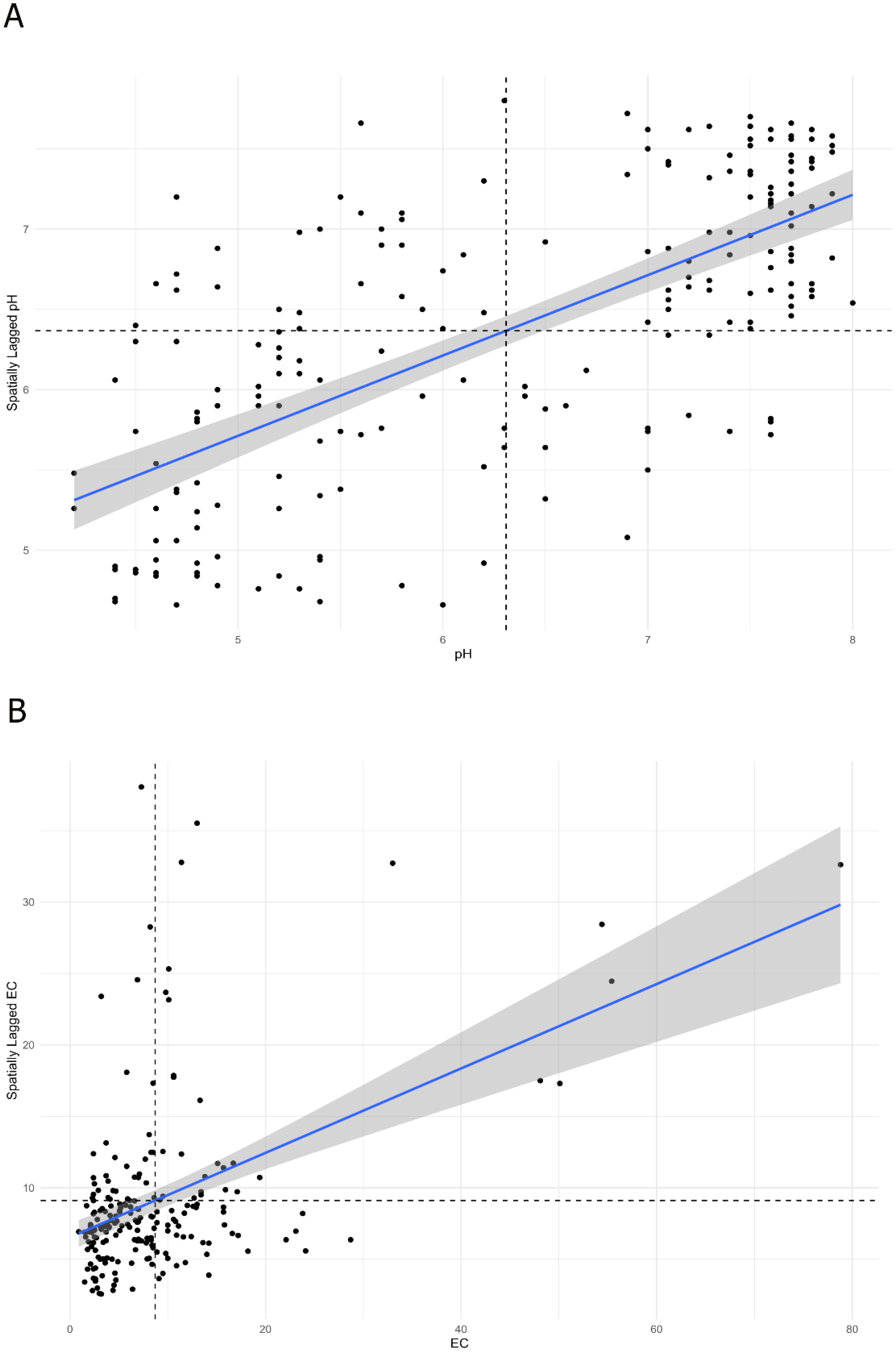
Figure 5. (A) Moran scatterplot for soil pH. (B) Moran scatterplot for electrical conductivity.

A LISA cluster classification map was used to identify distinct spatial clustering patterns for both variables. For pH (Figure 6A), High-High (H-H) clusters revealed localized areas of extremely high values surrounded by similarly elevated neighbors, demonstrating strong positive spatial autocorrelation. Low-Low (L-L) clusters exhibited an inverse pattern, with below-average pH values spatially concentrated in coherent regions, also indicating positive autocorrelation. Spatial outliers, marked by High-Low (H-L) and Low-High (L-H) clusters, highlighted situations where high or low values were isolated and bordered by contrasting values. These clusters denote negative spatial autocorrelation and could indicate problematic data points or areas of transition. In contrast, EC displayed markedly different spatial clustering behavior (Figure 6B), with only sparse H-H and L-H clusters detected across the study area. Large portions of the EC dataset showed non-significant spatial autocorrelation, suggesting more random or weakly structured spatial patterns that warrant additional investigation to understand the underlying processes driving this distribution.

Figure 6

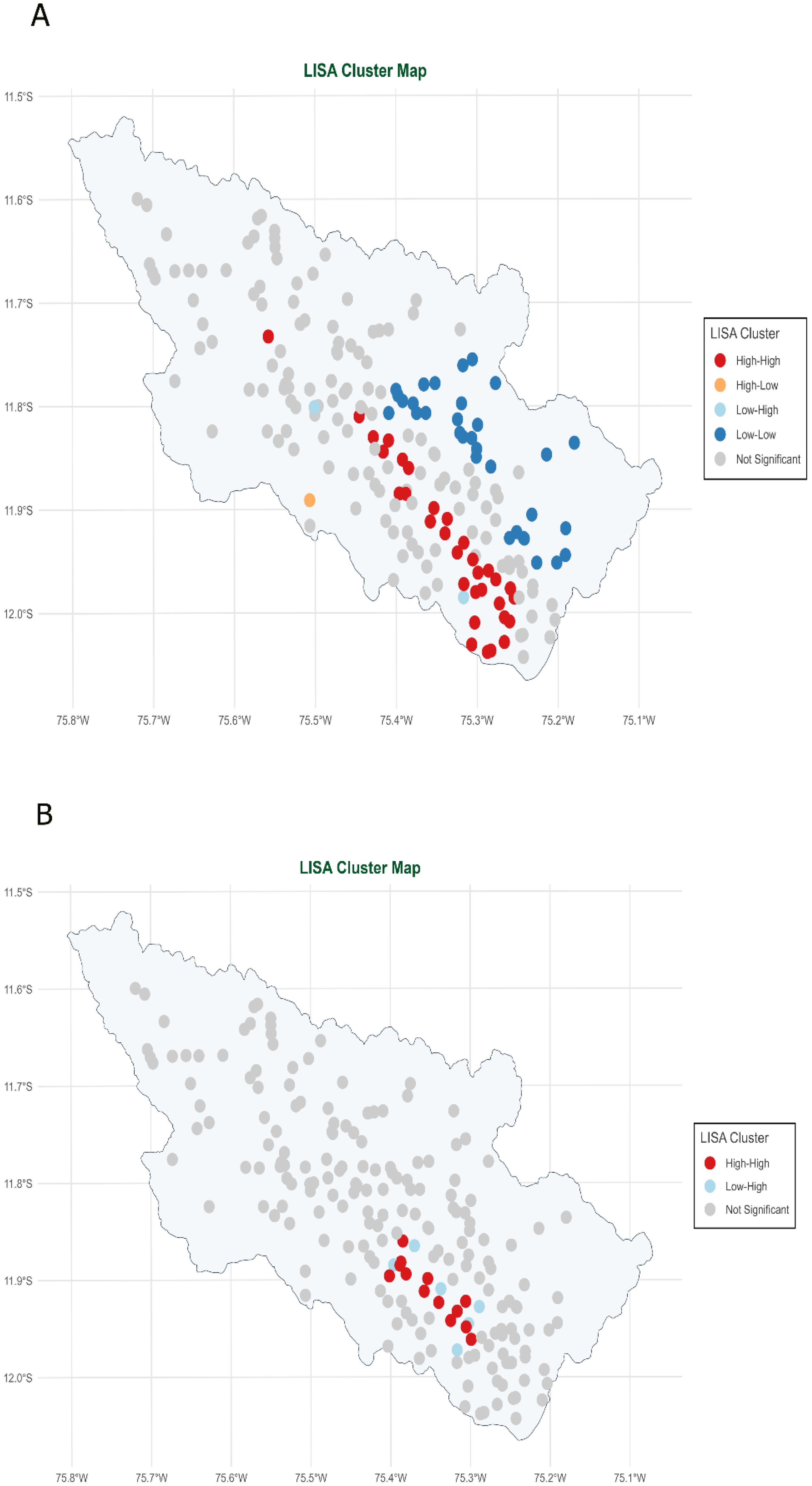
Figure 6. (A) Local Indicators of Spatial Autocorrelation(LISA) cluster map for soil pH. (B) Local Indicators of Spatial Autocorrelation(LISA) cluster map for electrical conductivity.

3.3 Correlation analysis between soil properties and environmental predictors

Strong internal correlations within variable clusters were observed through correlation matrix (Figure 7), suggesting that multicollinearity may be present in the dataset. High positive correlations represented with larger circles were detected among the moisture variables (VWC_FC, VWC_PMP, and VWC_SAT), indicating that similar aspects of soil water content were being assessed by these measures. Potential redundancy in vegetation measurements was suggested by the moderate to strong correlations found among vegetation indices (GNDVI, MSAVI, NDVI, and SAVI). Similar correlation patterns were observed for topographic variables (elevation, slope, and TPI), indicating comparable spatial relationships. In contrast, diverse correlation patterns (smaller circles) were exhibited by variables such as clay, silt, sand, and topographic indices (TRI, TWI), suggesting that unique insights could contribute to model development by these parameters. In addition, we can appreciate “X” symbol, which indicates correlations that are not statistically significant at the 0.10 significance level (90% confidence).

Figure 7

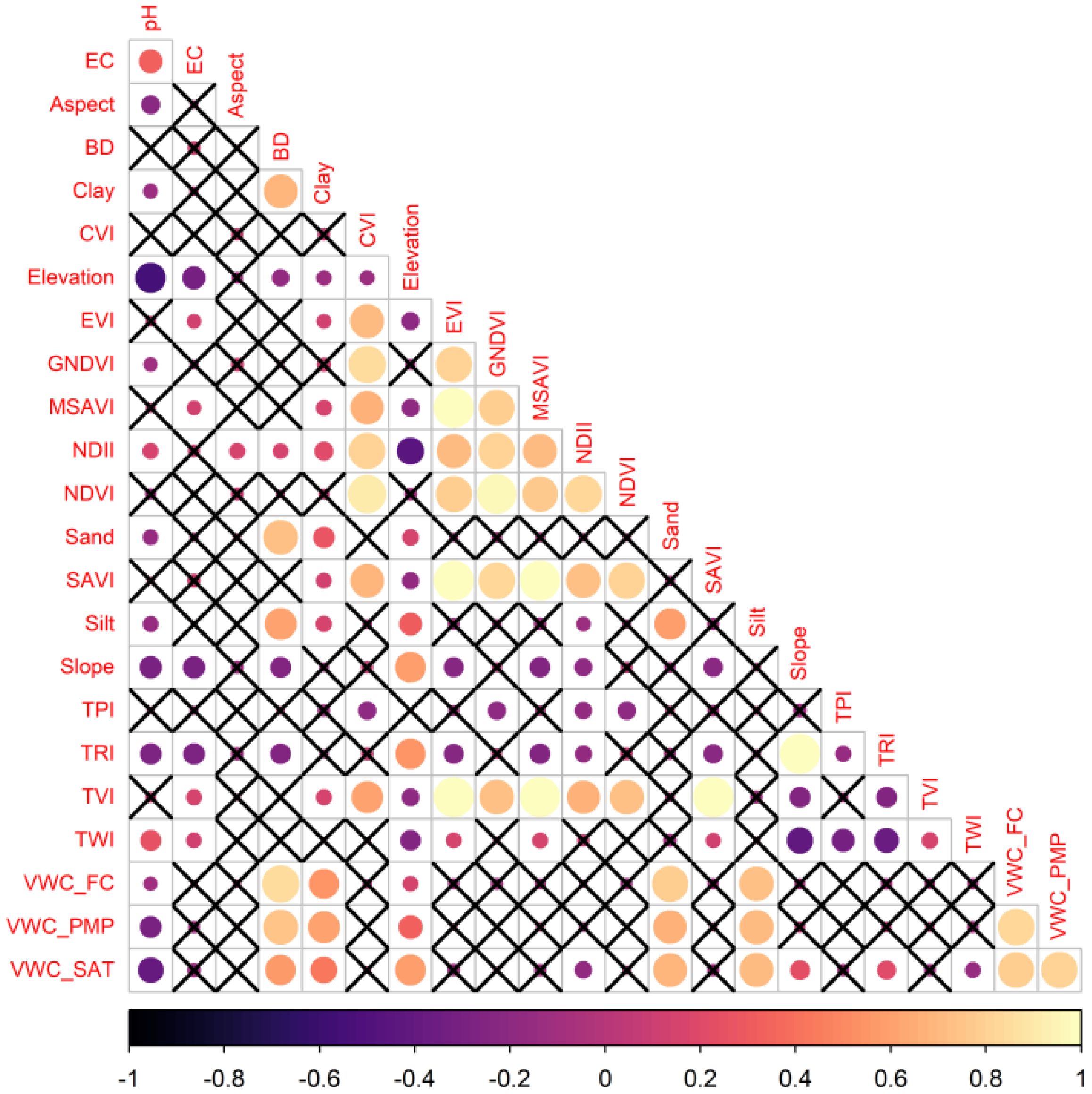
Figure 7. Correlation matrix heatmap among electrical conductivity (EC), aspect, bulk density (BD), clay, chlorophyll vegetation index (CVI), elevation, enhanced vegetation index (EVI), green normalized difference vegetation index (GNDVI), modified soil-adjusted vegetation index (MSAVI), normalized difference infrared index (NDII), normalized difference vegetation index (NDVI), sand, soil adjustment vegetation index (SAVI), silt, slope, topographic position index (TPI), topographic ruggedness index (TRI), triangular vegetation index (TVI), topographic wetness index (TWI), volumetric water content at field capacity (VWC_FC), volumetric water content at permanent wilting point (VWC_PMP), and volumetric water content at saturation (VWC_SAT) variables.

3.4 Predictions with machine learning and ensemble approaches

The relative contributions of environmental and soil covariates to soil pH and EC prediction were assessed through feature importance analysis comparing RF and XGBoost models. For pH prediction (Figure 8A), ten features were evaluated: Elevation, TRI, VWC_PWP (Volumetric Water Content at Permanent Wilting Point), Aspect, BD, Clay, TWI, CVI, EVI, and NDVI. Elevation emerged as the dominant predictor in both models, demonstrating the highest normalized importance (>90%) and underscoring its critical role in pH spatial distribution. Notable differences between models were observed, with RF consistently assigning higher importance to most features compared to XGBoost, particularly for TRI, VWC_PWP, and BD. For EC prediction (Figure 8B), the feature set was expanded to include SAVI, GNDVI, NDII, TPI, Sand, Silt, and VWC_SAT (Volumetric Water Content at Saturation). Elevation and Aspect dominated the prediction framework, accounting for over 90% and 80% of feature importance respectively in both models. Model-specific preferences were again evident, with RF assigning greater importance to TRI, EVI, and SAVI, while XGBoost emphasized Aspect and BD more heavily.

Figure 8

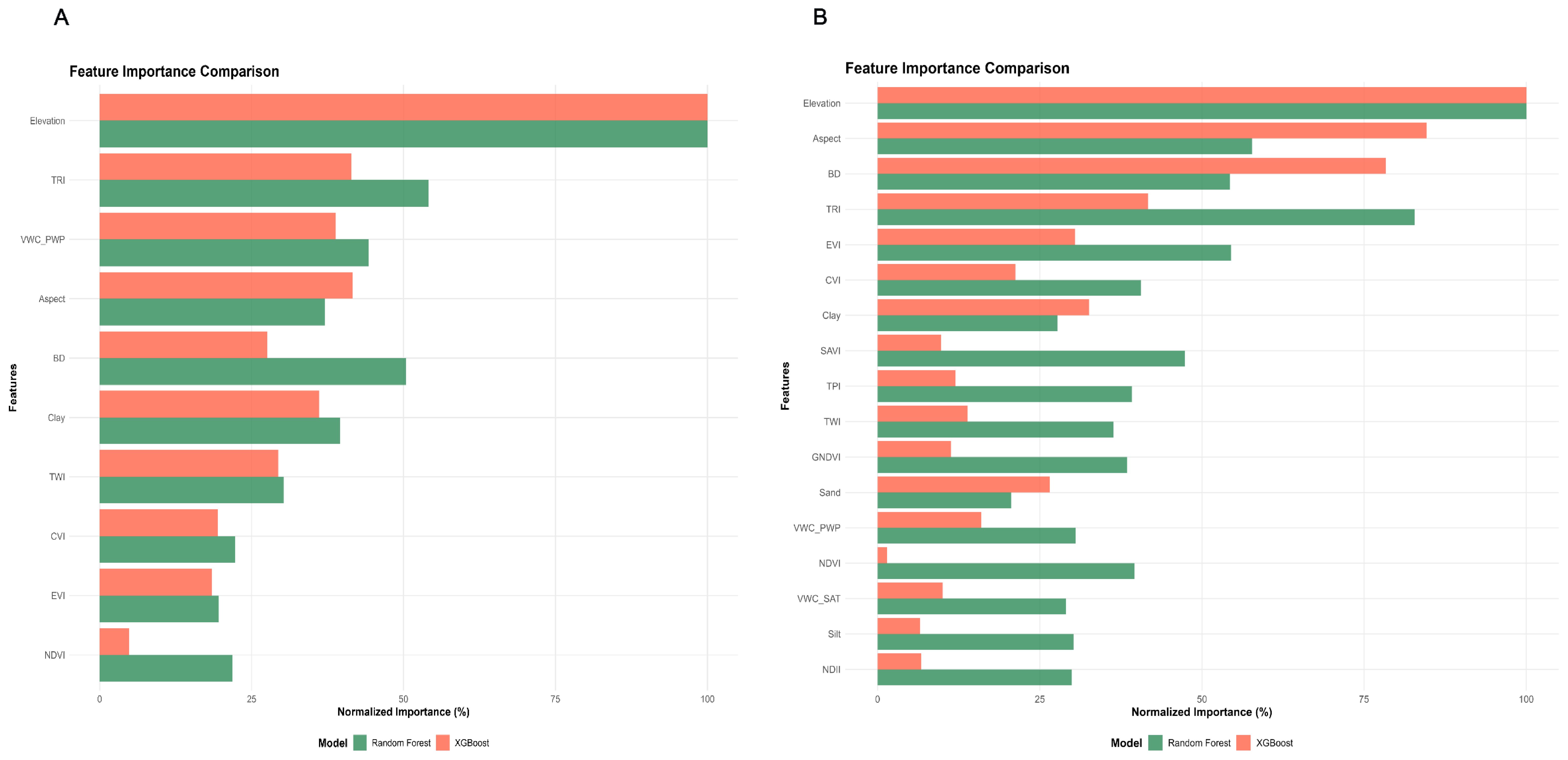
Figure 8. (A) Feature importance comparison of Random Forest and Extreme Gradient Boosting for pH. (B) Feature importance comparison of Random Forest and Extreme Gradient Boosting for electrical conductivity.

The raster maps in Figure 9 were generated by all ML models following training on observed pH data. Two further maps were created using ensemble techniques. Distinct spatial patterns in pH prediction were observed across the four ML models. RF and XGBoost models demonstrated similar predictive patterns, identifying extensive areas of neutral pH conditions (6.0-7.5) predominantly in flat terrain, while mountainous regions were characterized by acidic conditions (pH< 6.0). By comparison, the SVM model predicted alkaline pH values (7.5-9.0) for the majority of the study area, whereas neutral conditions appeared broadly, regardless of elevation or topographic location. The ANN model exhibited the most variable predictions, generating a heterogeneous spatial pattern with pH values fluctuating between acidic and alkaline conditions across the landscape without clear topographic associations.

Figure 9

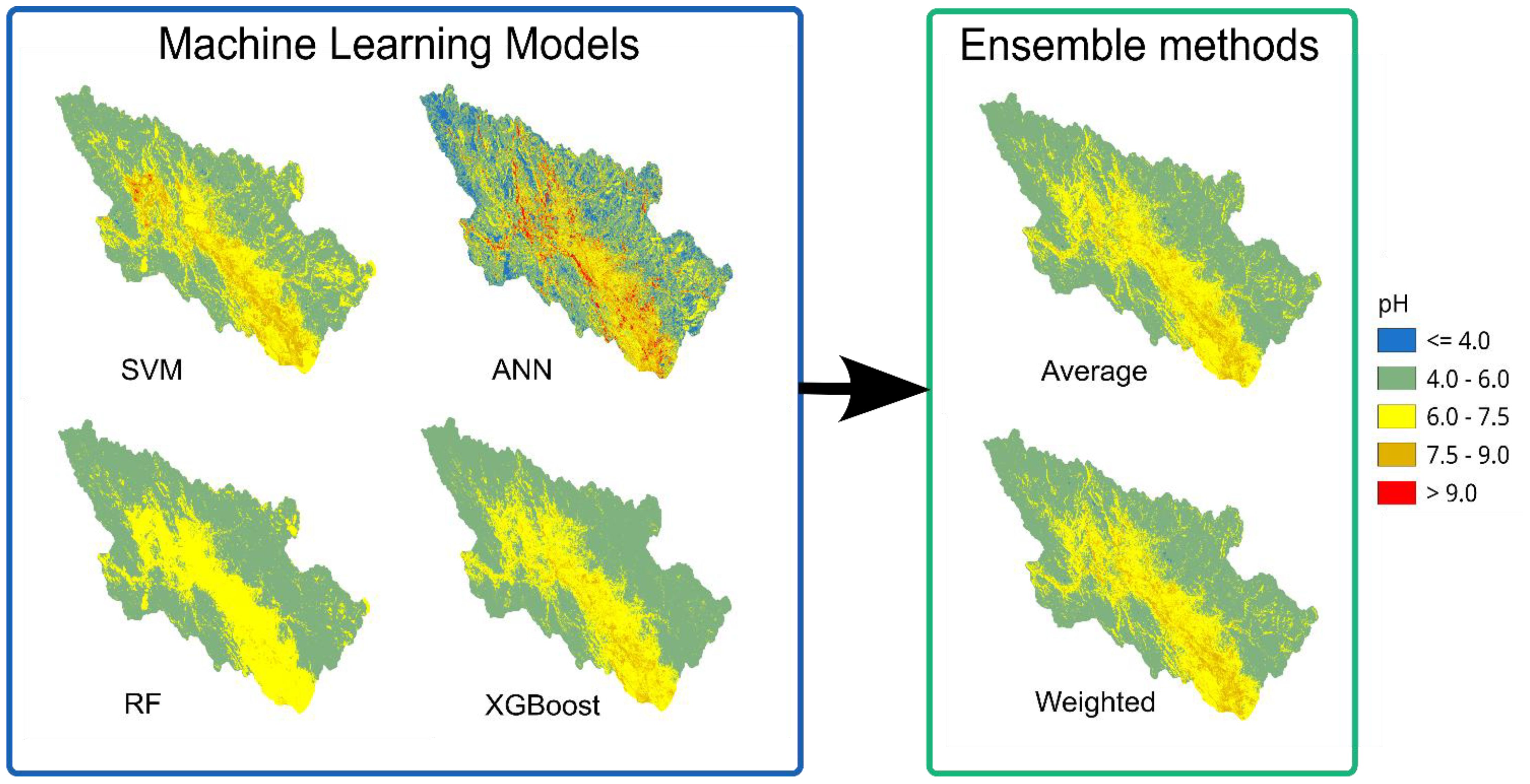
Figure 9. Spatial predictions of pH using all individual models and ensemble frameworks.

Additional EC map groups were generated by the same ML models and subsequently combined through ensemble methods to produce two additional maps (Figure 10). Moderate predictions with balanced distribution across the 4.0-15.0 mS·m^-¹ range were produced by SVM, with localized high-conductivity areas being identified. In contrast, the most extreme predictions were exhibited by ANN, with extensive areas exceeding 20.0 mS·m^-¹ being concentrated primarily in the central and southern portions of the study area. Predictions from the RF model were characterized as conservative, with values in 4.0–10.0 mS·m^-¹ range, though some areas with highly elevated EC levels were included, suggesting that a more stable prediction pattern was being generated. The most restrained predictions with minimal extreme values were produced by XGBoost, indicating that the most conservative approach among the four tested algorithms was being employed. Very similar patterns were exhibited by both ensemble methods, with individual model predictions being successfully balanced and extreme values observed in the ANN model being effectively smoothed out.

Figure 10

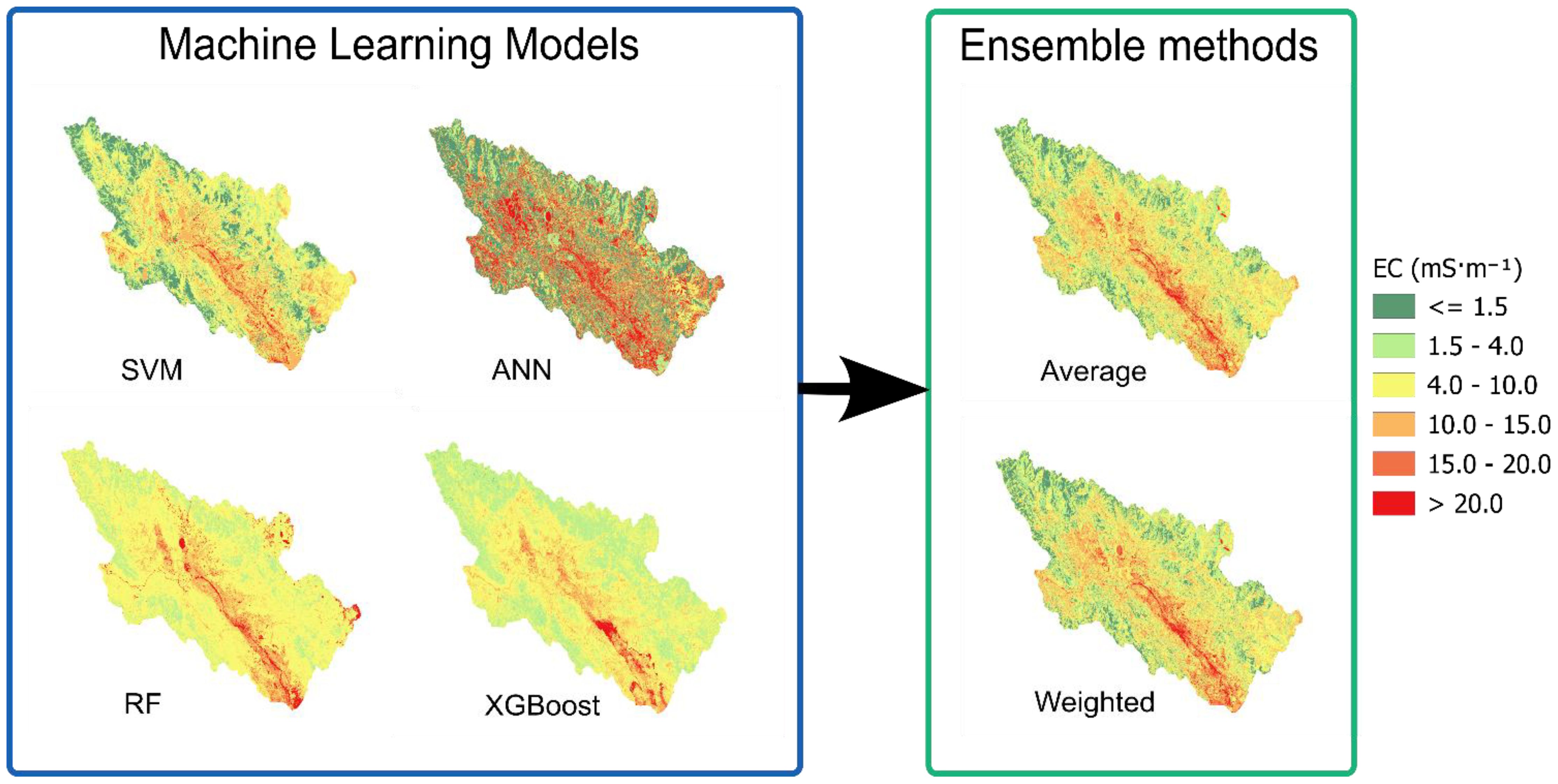
Figure 10. Spatial predictions of electrical conductivity(EC) using all individual models and ensemble frameworks.

3.5 Uncertainty estimation and assessment of models

The coefficient of variation (CV) maps revealed striking differences in ensemble model uncertainty between predictions of soil pH and EC across the study area. For pH predictions, excellent model agreement was demonstrated across 70-80% of the study area (Figure 11A), with CV values ≤ 0.10 dominating the spatial pattern. Moderate uncertainty zones (CV = 0.10-0.25) appeared as scattered patches, likely representing topographic transition areas with complex pH gradients. High uncertainty areas (CV = 0.25-0.50) were relatively rare, occurring as isolated patches under unique environmental conditions. In contrast, EC predictions exhibited widespread model disagreement, with extensive regions showing CV values between 0.25 and 0.50 across large portions of the landscape (Figure 11B). Large contiguous areas with CV > 0.50 indicated high uncertainty clusters, potentially reflecting complex geochemical processes that were inadequately captured by available predictors. Consensus areas (CV ≤ 0.10) were limited and fragmented, appearing as scattered patches throughout the study area.

Figure 11

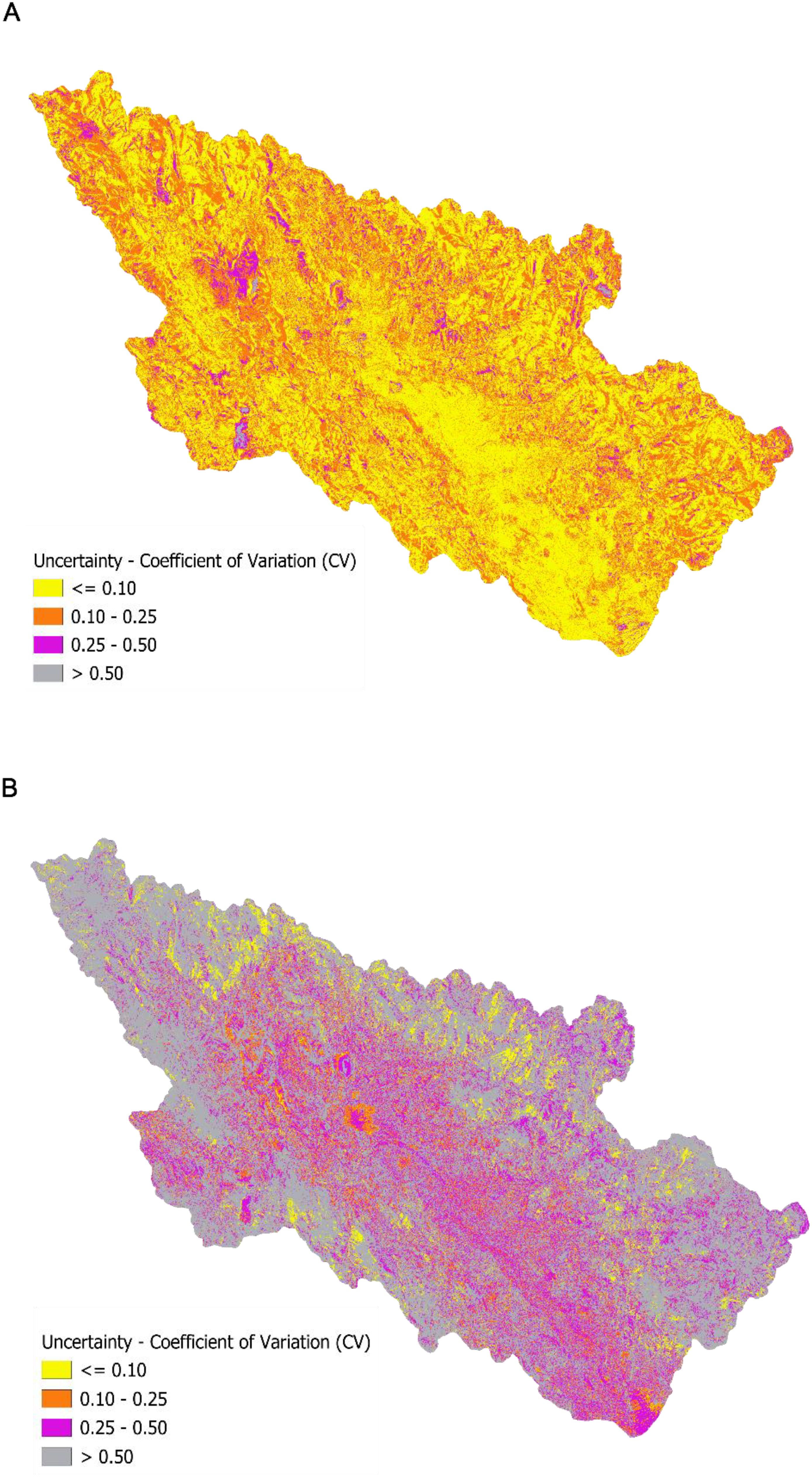
Figure 11. (A) Relative disagreement between ensemble weighted model predictions according to coefficient of variation maps for pH. (B) Relative disagreement between ensemble weighted model predictions according to coefficient of variation maps for electrical conductivity.

Performance metrics for the four machine learning models (SVM, ANN, RF, XGBoost) and their ensemble approaches (Average and Weighted) in predicting soil pH and EC are presented in Table 4. For soil pH prediction, substantial variation in model effectiveness was observed among individual algorithms. XGBoost demonstrated superior performance with the highest R² (0.993) and lowest MAE (0.849), while RF achieved the lowest RMSE (1.002). Conversely, ANN exhibited the poorest performance across all metrics, recording the highest RMSE (1.854) and MAE (1.432). Each ensemble approach consistently outperformed all individual models, with significant improvements in error reduction and prediction accuracy. The ensemble methods effectively leveraged the strengths of individual algorithms while mitigating their respective weaknesses, resulting in more robust and reliable soil property predictions. The Weighted Ensemble proved to be the superior model overall, achieving the lowest RMSE (0.282) and MAE (0.214), along with a very strong R² of 0.946. This represents a remarkable 72% reduction in RMSE compared to the best individual model (RF) and a 75% reduction in MAE compared to the best individual model (XGBoost), clearly demonstrating the power of the ensemble approach in generating more accurate and reliable pH predictions.

Table 4

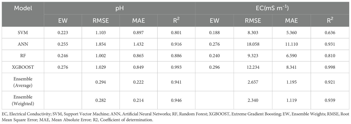
Table 4. Performance of machine learning models and ensemble approaches.

A similar trend was observed for the prediction of soil EC. Among the individual models, performance was inconsistent. While the SVM model produced the lowest RMSE (8.303) and MAE (5.36), its R² value was low (0.636), indicating a poor fit. Conversely, the XGBoost model achieved a near-perfect R² of 0.998, but with higher error values than SVM. The ANN model had the highest error metrics by a significant margin. Once again, the ensemble approach resolved these inconsistencies and delivered superior performance. The Weighted Ensemble model was the clear winner, achieving the lowest RMSE (2.340) and MAE (1.119), while maintaining a high R² of 0.939. This represents a 72% decrease in RMSE compared to the best individual model (SVM). These results show that ensemble methods leverage the strengths of their component models to produce a final model characterized by high accuracy (low error) and strong explanatory power (high R²).

4 Discussion

4.1 Measures of soil properties and their spatial behavior

The measured soil pH in our study area ranged from 4.2 to 8.0 (Table 1) and aligns with typical Andean soil gradients, which vary from acidic volcanic to neutral or alkaline valley soils. Research demonstrates that Peruvian Andean soils exhibit a distinct pH gradient, with topsoil displaying moderately acidic conditions (pH 5.5) while deeper layers remain slightly alkaline (pH 7.4) (914). At a depth of 30 cm, pH values range between 3.9 and 5.8 (92), confirming the acidic nature of surface and subsurface horizons. Our results also showed a broad range of EC (0.9–78.8 mS·m^-¹). While some locations exhibited high salinity, the low average EC values suggest that most soils were non-saline and thus structurally unstable and prone to nutrient deficiencies (3).

Spatial autocorrelation analysis revealed non-random distributions for both pH and EC (Table 2). The pronounced clustering of pH values suggests the influence of extensive, contiguous zones characterized by dominant soil types or parent materials, factors that, according to Eger et al. (93), exert a stronger influence on pH than climate. Moreover, high-resolution topographic data have been shown to reliably predict variations in topsoil pH (94). EC also displayed spatial clustering, though less pronounced than pH, suggesting that pH distribution factors have a more substantial and consistent influence over larger areas. EC appears more susceptible to localized factors such as variations in moisture content, agricultural inputs distribution, or measurement inconsistencies, as the interpretation of apparent electrical conductivity readings varies by location and soil type (95).

The integration of Moran scatter plots (Figure 5) with LISA cluster classification maps (Figure 6) confirms these patterns and supports the use of ML approaches that incorporate spatial coordinates or covariates to explain ecosystem condition variation. This approach is consistent with previous research demonstrating that incorporating spatial information enhances accuracy by addressing spatial autocorrelation (96). Understanding these spatial patterns is crucial for designing efficient sampling strategies and targeting management interventions (97). Performance remains context-dependent: robust for pH but less effective for EC. Although Local Moran and G-statistics are useful for identifying clusters, they do not provide significance testing, unlike heuristic methods (98).

The implications of our results highlight the importance of spatial patterns in EC and pH within agricultural settings, given their strong correlation with soil nutrients. Research indicates that an increase of one unit in potassium results in an approximate rise of 0.24 units in EC, whereas a similar increment in magnesium leads to an increase of about 0.68 units in EC, in contrast, an increase of P by one unit was related to a decrease of EC by 0.3 units (99). Under this line, other studies reveal that long-term annual manure applications in Andean agriculture have proven practical and beneficial, maintaining soil pH and increasing EC levels (100). Also, it was revealed that there were inconsistent relationships between soil salinity and altitude, with variations across different ecosystems. Some studies report a decrease in EC at higher elevations, a trend associated with greater leaching (101). Conversely, research in tropical rainforests indicates a significant increase in EC with altitude, suggesting that cooler high-altitude temperatures may inhibit nutrient removal processes, leading to ion accumulation (102). While another study found no significant difference in EC among sites at varying altitudes, lower altitudes exhibited higher pH levels, suggesting that factors including parent material, temperature, and precipitation may be more influential than altitude (103).

4.2 Correlations analysis between predictors

Multicollinearity could be a problem, especially with the VWC cluster variables, as shown in the correlation analysis in Figure 7. Models such as RF and XGBoost exhibit greater capacity to address multicollinearity compared to linear models (104, 105). Soil texture variables (clay, silt, and sand) showed high intercorrelation; using a single variable (i.e., clay) is preferable due to spectral similarities and the indistinctness of hillslopes (106). Similarly, one or two vegetation indices suffice to avoid redundancy while capturing plant health. Multi-index analyses remain valuable for ecosystem monitoring (107). When EC is the target variable, the analysis reveals moderately positive relationships with certain soil properties (clay content, some VWC measures), while relationships with terrain attributes are weak. This aligns with the typically strong correlation between EC and soil moisture influenced by soil texture, where higher EC usually suggests more clay and less sand (99). Previous studies have confirmed that EC exhibits a relatively strong spatial correlation with both clay percentage and pH (108), and the soil organic carbon to clay-sized particle ratio is strongly influenced by soil pH (109). Our research identified a negative correlation between altitude and pH, corroborating studies that show higher altitudes significantly reduce pH (p< 0.001) (110), although climate and mineralogy complicate quantification (111). When examining the relationship between pH and EC, research suggests a weak, negative correlation between pH and EC (99).

4.3 Feature importance analysis to machine learning

Topographic variables, particularly Elevation, TWI, Aspect, and TPI, were the most powerful predictors in both RF and XGBoost models (Figure 8). Elevation ranks as the most important variable because it serves as a powerful proxy controlling multiple environmental processes at the landscape scale (112). Processes influenced by climate (temperature and rainfall) systematically change with elevation (113, 114), while TWI explicitly models the impact of downhill water flow on soil properties by identifying areas prone to water accumulation (115). Although topographic and soil conditions influence vegetation indices that measure plant health (116, 117), the connection between vegetation indices and our target variables is weakened by the overriding influence of long-term landscape processes. Researchers employ remote sensing algorithms to analyze vegetation indices across different land areas, enabling the identification of soil variations affecting plant growth (118).

4.4 Use of ensemble approach for predictions purposes

The ensemble approach improves upon traditional bagging methods, such as RF, by integrating the unique strengths of different algorithm families to more effectively model complex spatial patterns. The use of an averaged ensemble produces spatially more realistic results by balancing individual model predictions, effectively smoothing extreme values in individual models (particularly ANN models for pH) while preserving spatial patterns identified by other models (Figure 9). This is compressible because ensemble learning is so strong and effective, it improves how well models predict. In recent years, ensemble learning has become a significant research focus, resulting in more studies across diverse application areas (119). Since the weighted ensemble and simple average produced nearly identical results, either the weights were evenly distributed across models or model performance was consistent during validation. As an example about their advantages of using this approach, a nested optimization algorithm, which tuned hyperparameters and determined optimal weights for combining ensembles, was used with a stacked ensemble method and weighted average to minimize variance and maps from the EC consistently show similar spatial patterns across all methods (Figure 10), with higher values concentrated in the lower-elevation central valley and lower values in the highlands. The ensemble approaches provide more spatially coherent predictions with smoother transitions between EC classes, reducing the pixelated or noisy patterns visible in some individual models. Recent studies have demonstrated that ensemble learning has become a significant research focus, particularly with stacked ensemble methods that utilize nested optimization algorithms to simultaneously tune hyperparameters and determine the optimal weights for combining models. This approach effectively minimizes both variance and bias (120). Numerous other studies further confirm that ensemble models provide more reliable and versatile prediction accuracy, thereby enhancing decision-making across various applications (36, 121–124).

4.5 Analysis of predictive uncertainty

The stark differences between pH and EC uncertainty maps (Figure 11) demonstrate that pH is inherently more predictable than EC in Andean soils, likely because pH is more directly controlled by parent material and basic soil-forming processes, which are well-captured by topographic and climatic predictors (94). The high EC uncertainty explains the dramatic differences observed between individual models, particularly the extreme predictions of ANN models. These uncertainty maps identify high-uncertainty EC areas as priority locations for additional sampling to improve model accuracy and reduce prediction uncertainty in risk assessment. Alternatively, a study used auxiliary soil data and a general linear model to reduce EC uncertainty (125). By contrast, we can confidently use pH predictions to inform most management decisions. The significant differences in spatial uncertainty patterns between pH and EC predictions are explained and validated by the results in Table 3, which supports our ensemble approach. Some models demonstrated high R² values for some individual models (especially XGBoost and ANN), combined with high error metrics, suggesting that these models may be overfitting or producing unrealistic, extreme predictions, particularly evident in the spatial maps of the ANN model. XGBoost delivers strong performance in predicting soil properties, as supported by studies showing RMSEs of 1.03–1.09 for pH and 26.53 mg/kg for phosphorus, consistent with dataset variability and highlighting some limits with nutrient prediction (126). According to recent studies, XGBoost models outperform traditional methods in predicting soil freezing characteristic curves (127), and soil organic matter (128). On the other hand, ensemble methods effectively combine model strengths and reduce individual weaknesses, which is especially valuable in EC where significant disagreement between models occurs. EC prediction remains more challenging than pH, as evidenced by higher MAE values, even in ensemble methods, which explains the higher uncertainty patterns in your CV maps (Figure 11). Our fivefold cross-validation tuning process was surpassed by the performance of the models. This method verifies that the chosen hyperparameters are not only effective on the training data but also demonstrate robust generalization to unseen data, thus reducing the risk of overfitting (36).

5 Conclusions

Andean soil pH and EC show substantial variability, where EC displays notably higher variability and positive skewness compared to pH. We identified distinct spatial patterns using spatial autocorrelation analysis (Moran’s I, Geary’s C, LISA), which shows strong, statistically significant spatial clustering for pH, indicating dominant landscape-level controls. In contrast, EC exhibits moderate spatial autocorrelation, suggesting its distribution is more influenced by localized factors.

Correlation analysis reveals significant multicollinearity among groups of related variables, such as soil moisture indices, VIs, and soil texture. Topographic variables, especially Elevation, are the most influential predictors for both pH and EC in machine learning models, like RF and XGBoost, serving as proxies for combined environmental processes. Soil texture variables and certain VIs provide unique information but must be selected carefully to prevent redundancy.

Ensemble models generated the most spatially coherent and realistic maps for both pH and EC, outperforming any individual model. Among the standalone models, XGBoost and RF performed best for pH, while SVM had the best error metrics for EC. The ANN models consistently performed the poorest, exhibiting unrealistic spatial predictions and potential overfitting. The success of the ensemble approach lies in its ability to balance these individual predictions, effectively smoothing extreme values from models like ANN to produce more reliable and accurate maps with smoother transitions between value classes. Ensemble approaches (Average and Weighted) consistently and significantly outperform all individual ML models (SVM, ANN, RF, XGBoost) for predicting both soil pH and EC. The Weighted Ensemble achieved the highest accuracy, demonstrating a substantial error reduction of approximately 72% in RMSE compared to the best individual models, and strong explanatory power (R² > 0.93).

Through uncertainty assessment with CV maps, a significant difference is observed in the values of pH and EC. The predictions for pH are quite certain (low CV) over most of the area, but the EC predictions are widely uncertain (high CV), suggesting that predicting EC accurately within this framework is inherently difficult. High-uncertainty EC zones are priority targets for future sampling. The strong spatial structure of pH and the demonstrated high accuracy of its ensemble predictions make it reliable for informing soil management decisions. The higher uncertainty associated with EC predictions necessitates caution in their application for risk assessment but identifies specific areas needing further investigation. Understanding these spatial patterns is crucial for efficient sampling and targeted interventions.

As a recommendation for ensemble modeling, implementing methods with optimized weighting schemes is highly advised for DSM of spatially autocorrelated properties, such as pH and EC. This approach effectively leverages the strengths of different models and reduces individual weaknesses, resulting in improved accuracy and robustness. Lightweight ensemble frameworks also show potential for real-time applications.

Data availability statement

The raw data supporting the conclusions of this article will be made available by the authors, without undue reservation.

Author contributions

CC-I: Conceptualization, Investigation, Writing – original draft, Data curation, Software, Formal Analysis, Methodology. AB: Writing – original draft, Visualization, Data curation. SP: Writing – review & editing, Validation.

Funding

The author(s) declare financial support was received for the research and/or publication of this article. This research was funded by the INIA project CUI 2487112 “Mejoramiento de los servicios de investigación y transferencia tecnológica en el manejo y recuperación de suelos agrícolas degradados y aguas para riego en la pequeña y mediana agricultura en los departamentos de Lima, Áncash, San Martín, Cajamarca, Lambayeque, Junín, Ayacucho, Arequipa, Puno y Ucayali”.

Acknowledgments

To the personnel of the Soil, Water, and Foliars Laboratory (LABSAF) at the Santa Ana Agrarian Experimental Station (EEA).

Conflict of interest

The authors declare that the research was conducted in the absence of any commercial or financial relationships that could be construed as a potential conflict of interest.

Generative AI statement

The author(s) declare that no Generative AI was used in the creation of this manuscript.

Any alternative text (alt text) provided alongside figures in this article has been generated by Frontiers with the support of artificial intelligence and reasonable efforts have been made to ensure accuracy, including review by the authors wherever possible. If you identify any issues, please contact us.

Publisher’s note

All claims expressed in this article are solely those of the authors and do not necessarily represent those of their affiliated organizations, or those of the publisher, the editors and the reviewers. Any product that may be evaluated in this article, or claim that may be made by its manufacturer, is not guaranteed or endorsed by the publisher.

References

1. Fausak LK, Bridson N, Diaz-Osorio F, Jassal RS, and Lavkulich LM. Soil health – a perspective. Front Soil Sci. (2024) 4:1462428. doi: 10.3389/fsoil.2024.1462428

Crossref Full Text | Google Scholar

2. Singh A, Pandey AK, and Singh U. Assessment of soil fertility of some villages of mahishi block, saharsa, bihar. J Exp Agric Int. (2022) 44(2):55–60. doi: 10.9734/jeai/2022/v44i230798

Crossref Full Text | Google Scholar

3. Smith JL and Doran JW. Measurement and use of pH and electrical conductivity for soil quality analysis. In: Methods for assessing soil quality. Madison, Wisconsin (USA): John Wiley & Sons, Ltd.(1997). doi: 10.2136/sssaspecpub49.c10

Crossref Full Text | Google Scholar

4. El-Ramady H, Prokisch J, Mansour H, Bayoumi YA, Shalaby TA, Veres S, et al. Review of crop response to soil salinity stress: possible approaches from leaching to nano-management. Soil Syst. (2024) 8:1. doi: 10.3390/soilsystems8010011

Crossref Full Text | Google Scholar

5. Trejo-Téllez LI. Salinity stress tolerance in plants. Plants. (2023) 12:20. doi: 10.3390/plants12203520

PubMed Abstract | Crossref Full Text | Google Scholar

6. Corwin DL and Yemoto K. Salinity: electrical conductivity and total dissolved solids. Soil Sci Soc America J. (2020) 84:1442–61. doi: 10.1002/saj2.20154

Crossref Full Text | Google Scholar

7. Rieder L, Amann T, and Hartmann J. Soil electrical conductivity as a proxy for enhanced weathering in soils. Front Climate. (2024) 5:1283107. doi: 10.3389/fclim.2023.1283107

Crossref Full Text | Google Scholar

8. Corwin DL and Scudiero E. Field-scale apparent soil electrical conductivity. Soil Sci Soc America J. (2020) 84:1405–41. doi: 10.1002/saj2.20153

Crossref Full Text | Google Scholar

9. Yüzügüllü O, Fajraoui N, and Liebisch F. Soil texture and pH mapping using remote sensing and support sampling. IEEE J Selected Topics Appl Earth Observations Remote Sens. (2024) 17:12685–705. doi: 10.1109/JSTARS.2024.3422494

Crossref Full Text | Google Scholar

10. Adeniyi OD, Bature H, and Mearker M. A systematic review on digital soil mapping approaches in lowland areas. Land. (2024) 13:3. doi: 10.3390/land13030379

Crossref Full Text | Google Scholar

11. Samieifard R, Drohan PJ, and Heidari A. Modeling soil electrical conductivity using machine learning: implications for sustainable land use in saline coastal regions. J Geogr Cartography. (2025) 8:2. doi: 10.24294/jgc11427

Crossref Full Text | Google Scholar

12. Searle R, McBratney A, Grundy M, Kidd D, Malone B, Arrouays D, et al. Digital soil mapping and assessment for Australia and beyond: A propitious future. Geoderma Regional. (2021) 24:e00359. doi: 10.1016/j.geodrs.2021.e00359

Crossref Full Text | Google Scholar

13. Emadi M and Baghernejad M. Comparison of spatial interpolation techniques for mapping soil pH and salinity in agricultural coastal areas, northern Iran. Arch Agron Soil Sci. (2014) 60:1315–27. doi: 10.1080/03650340.2014.880837

Crossref Full Text | Google Scholar

14. Rodrigues AF, Latawiec AE, Reid BJ, Solórzano A, Schuler AE, Lacerda C, et al. Systematic review of soil ecosystem services in tropical regions. R Soc Open Sci. (2021) 8:201584. doi: 10.1098/rsos.201584

PubMed Abstract | Crossref Full Text | Google Scholar

15. Wang J, Zhen J, Hu W, Chen S, Lizaga I, Zeraatpisheh M, et al. Remote sensing of soil degradation: progress and perspective. Int Soil Water Conserv Res. (2023) 11:429–54. doi: 10.1016/j.iswcr.2023.03.002

Crossref Full Text | Google Scholar

16. Hengl T, de Jesus JM, Heuvelink GBM, Ruiperez Gonzalez M, Kilibarda M, Blagotić A, et al. SoilGrids250m: global gridded soil information based on machine learning. PloS One. (2017) 12:e0169748. doi: 10.1371/journal.pone.0169748

PubMed Abstract | Crossref Full Text | Google Scholar

17. Westhuizen Svd, Heuvelink GBM, and Hofmeyr DP. Multivariate random forest for digital soil mapping. Geoderma. (2023) 431:116365. doi: 10.1016/j.geoderma.2023.116365

Crossref Full Text | Google Scholar

18. Hateffard F, Steinbuch L, and Heuvelink GBM. Evaluating the extrapolation potential of random forest digital soil mapping. Geoderma. (2024) 441:116740. doi: 10.1016/j.geoderma.2023.116740

Crossref Full Text | Google Scholar

19. Kumar A, Moharana PC, Jena RK, Malyan SK, Sharma GK, Fagodiya RK, et al. Digital mapping of soil organic carbon using machine learning algorithms in the upper brahmaputra valley of northeastern India. Land. (2023) 12:10. doi: 10.3390/land12101841

Crossref Full Text | Google Scholar

20. Vandana N, Suresh GJR, Mitran T, and Mahadevappa SG. Digital mapping of soil pH and electrical conductivity using geostatistics and machine learning. Int J Environ Climate Change. (2024) 14:273–86. doi: 10.9734/ijecc/2024/v14i23944

Crossref Full Text | Google Scholar

21. Suleymanov A, Abakumov E, Alekseev I, and Nizamutdinov T. Digital mapping of soil properties in the high latitudes of Russia using sparse data. Geoderma Regional. (2024) 36:e00776. doi: 10.1016/j.geodrs.2024.e00776

Crossref Full Text | Google Scholar

22. Bandak S, Movahedi-Naeini SA, Mehri S, and Lotfata A. A longitudinal analysis of soil salinity changes using remotely sensed imageries. Sci Rep. (2024) 14:10383. doi: 10.1038/s41598-024-60033-6

PubMed Abstract | Crossref Full Text | Google Scholar

23. Zhao Z-D, Zhao M-S, Lu H-L, Wang S-H, and Lu Y-Y. Digital mapping of soil pH based on machine learning combined with feature selection methods in east China. Sustainability. (2023) 15:17. doi: 10.3390/su151712874

Crossref Full Text | Google Scholar

24. Lu Q, Tian S, and Wei L. Digital Mapping of Soil pH and Carbonates at the European Scale Using Environmental Variables and Machine Learning. Sci Total Environ. (2023) 856:159171. doi: 10.1016/j.scitotenv.2022.159171

PubMed Abstract | Crossref Full Text | Google Scholar

25. Mantena S, Mahammood V, and Rao KN. Prediction of soil salinity in the upputeru river estuary catchment, India, using machine learning techniques. Environ Monit Assess. (2023) 195:1006. doi: 10.1007/s10661-023-11613-y

PubMed Abstract | Crossref Full Text | Google Scholar

26. Adhikari K, Smith DR, Collins H, Hajda C, Acharya BS, and Owens PR. Mapping within-field soil health variations using apparent electrical conductivity, topography, and machine learning. Agronomy. (2022) 12:1019. doi: 10.3390/agronomy12051019

Crossref Full Text | Google Scholar

27. Corwin DL and Lesch SM. Apparent soil electrical conductivity measurements in agriculture. Comput Electron Agriculture Appl Apparent Soil Electrical Conductivity Precis Agric. (2005) 46:11–43. doi: 10.1016/j.compag.2004.10.005

Crossref Full Text | Google Scholar

28. Lu M, Hou Q, Qin S, Zhou L, Hua D, Wang X, et al. A stacking ensemble model of various machine learning models for daily runoff forecasting. Water. (2023) 15:7. doi: 10.3390/w15071265

Crossref Full Text | Google Scholar

29. Wang S, Wu Y, Li R, and Wang X. Remote sensing-based retrieval of soil moisture content using stacking ensemble learning models. Land Degradation Dev. (2023) 34:911–25. doi: 10.1002/ldr.4505

Crossref Full Text | Google Scholar

30. Mishra U, Gautam S, Riley WJ, and Hoffman FM. Ensemble machine learning approach improves predicted spatial variation of surface soil organic carbon stocks in data-limited northern circumpolar region. Front Big Data. (2020) 3:528441. doi: 10.3389/fdata.2020.528441

PubMed Abstract | Crossref Full Text | Google Scholar

31. Adeniyi OD, Brenning A, Bernini A, Brenna S, and Maerker M. Digital mapping of soil properties using ensemble machine learning approaches in an agricultural lowland area of lombardy, Italy. Land. (2023) 12:2. doi: 10.3390/land12020494

Crossref Full Text | Google Scholar

32. Taghizadeh-Mehrjardi R, Nabiollahi K, and Kerry R. Digital mapping of soil organic carbon at multiple depths using different data mining techniques in baneh region, Iran. Geoderma. (2016) 266:98–110. doi: 10.1016/j.geoderma.2015.12.003

Crossref Full Text | Google Scholar

33. Padarian J, Minasny B, and McBratney AB. Machine learning and soil sciences: A review aided by machine learning tools. SOIL. (2020) 6:35–52. doi: 10.5194/soil-6-35-2020

Crossref Full Text | Google Scholar

34. Cao Y, Liu G, Sun J, Bavirisetti DP, and Xiao G. PSO-stacking improved ensemble model for campus building energy consumption forecasting based on priority feature selection. J Building Eng. (2023) 72:106589. doi: 10.1016/j.jobe.2023.106589

Crossref Full Text | Google Scholar

35. Hajihosseinlou M, Maghsoudi A, and Ghezelbash R. Stacking: A novel data-driven ensemble machine learning strategy for prediction and mapping of pb-zn prospectivity in varcheh district, west Iran. Expert Syst Appl. (2024) 237:121668. doi: 10.1016/j.eswa.2023.121668

Crossref Full Text | Google Scholar

36. Tahmouresi MS, Niksokhan MH, and Ehsani AH. Enhancing spatial resolution of satellite soil moisture data through stacking ensemble learning techniques. Sci Rep. (2024) 14:25454. doi: 10.1038/s41598-024-77050-0

PubMed Abstract | Crossref Full Text | Google Scholar

37. Tao S, Zhang X, Chen J, Zhang Z, Kang X, and Qi W. Generating Surface Soil Moisture at the 30 m Resolution in Grape-Growing Areas Based on Stacked Ensemble Learning. Int J Remote Sens. (2024) 45:5385–424. doi: 10.1080/01431161.2024.2377228

Crossref Full Text | Google Scholar

38. Kara A, Pekel E, Ozcetin E, and Yıldız GB. Genetic algorithm optimized a deep learning method with attention mechanism for soil moisture prediction. Neural Computing Appl. (2024) 36:1761–72. doi: 10.1007/s00521-023-09168-7

Crossref Full Text | Google Scholar

39. Wang C, Xu X, Zhang Y, Cao Z, Ullah I, Zhang Z, et al. A stacking ensemble learning model combining a crop simulation model with machine learning to improve the dry matter yield estimation of greenhouse pakchoi. Agronomy. (2024) 14:1789. doi: 10.3390/agronomy14081789

Crossref Full Text | Google Scholar

40. Ballabio C. Spatial prediction of soil properties in temperate mountain regions using support vector regression. Geoderma. (2009) 151:338–50. doi: 10.1016/j.geoderma.2009.04.022

Crossref Full Text | Google Scholar

41. Baruck J, Nestroy O, Sartori G, Baize D, Traidl R, Vrščaj B, et al. Soil classification and mapping in the alps: the current state and future challenges. Geoderma. (2016) 264:312–31. doi: 10.1016/j.geoderma.2015.08.005

Crossref Full Text | Google Scholar

42. Dasgupta S, Debnath S, Das A, Biswas A, Weindorf DC, Li B, et al. Developing regional soil micronutrient management strategies through ensemble learning based digital soil mapping. Geoderma. (2023) 433:116457. doi: 10.1016/j.geoderma.2023.116457

Crossref Full Text | Google Scholar

43. Jena RK, Moharana PC, Dharumarajan S, Sharma GK, Ray P, Roy PD, et al. Spatial prediction of soil particle-size fractions using digital soil mapping in the north eastern region of India. Land. (2023) 12:1295. doi: 10.3390/land12071295

Crossref Full Text | Google Scholar

44. Carbajal M, Ramírez DA, Turin C, Schaeffer SM, Konkel J, Ninanya J, et al. From rangelands to cropland, land-use change and its impact on soil organic carbon variables in a Peruvian andean highlands: A machine learning modeling approach. Ecosystems. (2024) 27:899–917. doi: 10.1007/s10021-024-00928-7

PubMed Abstract | Crossref Full Text | Google Scholar

45. Rengma NS, Yadav M, Kalambukattu JG, and Kumar S. Machine learning-based digital mapping of soil organic carbon and texture in the mid-himalayan terrain. Environ Monit Assess. (2023) 195:994. doi: 10.1007/s10661-023-11608-9

PubMed Abstract | Crossref Full Text | Google Scholar

46. Angelini ME, Heuvelink GBM, and Kempen B. Multivariate mapping of soil with structural equation modelling. Eur J Soil Sci. (2017) 68:575–91. doi: 10.1111/ejss.12446

Crossref Full Text | Google Scholar

47. Dash PK, Panigrahi N, and Mishra A. Identifying opportunities to improve digital soil mapping in India: A systematic review. Geoderma Regional. (2022) 28:e00478. doi: 10.1016/j.geodrs.2021.e00478

Crossref Full Text | Google Scholar

48. Dimri AP, Yasunari T, Wiltshire A, Kumar P, Mathison C, Ridley J, et al. Application of regional climate models to the Indian winter monsoon over the western himalayas. Sci Total Environ. (2013) 468–469:S36–47. doi: 10.1016/j.scitotenv.2013.01.040

PubMed Abstract | Crossref Full Text | Google Scholar

49. Alaboz P. Model ensemble techniques of machine learning algorithms for soil moisture constants in the semi-arid climate conditions. Irrigation Drainage. (2025) 74:529–40. doi: 10.1002/ird.3037

Crossref Full Text | Google Scholar

50. Wu M, Dou S, Lin N, Jiang R, and Zhu B. Estimation and mapping of soil organic matter content using a stacking ensemble learning model based on hyperspectral images. Remote Sens. (2023) 15:19. doi: 10.3390/rs15194713

Crossref Full Text | Google Scholar

51. IPCC. Climate change 2021 – the physical science basis: working group I contribution to the sixth assessment report of the intergovernmental panel on climate change. 1st ed. Cambridge (United Kingdom) and New York, NY (USA): Cambridge University Press (2023). doi: 10.1017/9781009157896

Crossref Full Text | Google Scholar

52. WMO. State of the global climate 2021. Geneva, Switzerland: World Meteorological Organization (2022). Available online at: https://library.wmo.int/idurl/4/56300 (Accessed June 13, 2025).

Google Scholar

53. Castro A, Arriaga CD, Laura W, Cubas Saucedo F, Avalos G, López C, et al. Climas del Perú: mapa de clasificación climática nacional. In: Repositorio institucional - SENAMHI. Lima, Peru: Servicio Nacional de Meteorología e Hidrología del Perú (2021). Available online at: http://repositorio.senamhi.gob.pe/handle/20.500.12542/1336 (Accessed January 20, 2025).

Google Scholar

54. ANA, Consorcio Typsa - Tecnoma - Engecorps, and Grupo Inclam. Evaluación de recursos hídricos en la cuenca de Mantaro. Autoridad Nacional del Agua(2015). Available online at: https://repositorio.ana.gob.pe/handle/20.500.12543/36 (Accessed July 15, 2025).

Google Scholar

55. Gobierno Regional de Junín. Memoria Descriptiva. Zonificación Ecológica y Económica Del Departamento de Junin a Nivel Meso y Escala 1:100 000. Junín, Perú: Ministerio del Ambiente - MINAM (2015). Available online at: https://sinia.minam.gob.pe/documentos/memoria-descriptiva-zonificacion-ecologica-economica-departamento (Accessed February 10, 2025).

Google Scholar

56. INEI. Censos Nacionales 2017: XII de Población, VII de Vivienda y III de Comunidades Indígenas(2017). Available online at: https://censos2017.inei.gob.pe/pubinei/index.asp (Accessed July 11, 2025).

Google Scholar

57. Minasny B and McBratney AB. A conditioned latin hypercube method for sampling in the presence of ancillary information. Comput Geosciences. (2006) 32:1378–88. doi: 10.1016/j.cageo.2005.12.009

Crossref Full Text | Google Scholar

58. Roudier P, Hewitt AE, and Beaudette DE. “A conditioned Latin hypercube sampling algorithm incorporating operational constraints,” in Digital Soil Assessments and Beyond, 1st Edition. London: CRC Press (2012) p. 227–32. doi: 10.1201/b12728-48.

Crossref Full Text | Google Scholar

59. Roudier P. Clhs: A R package for conditioned latin hypercube sampling. Vienna, Austria: CRAN (The Comprehensive R Archive Network) (2011). doi: 10.32614/CRAN.package.clhs

Crossref Full Text | Google Scholar

60. ISO and DIN. Soil quality. Determination of the specific electrical conductivity. Geneva (Switzerland): International Organization for Standardization Geneva (1994).

Google Scholar

61. Rouse JW, Haas RH, Schell JA, and Deering DW. Monitoring vegetation systems in the great plains with ERTS. In: NASA. Goddard space flight center 3d ERTS-1 symp., vol. 1, sect. A Greenbelt, Maryland: NASA Goddard Space Flight Center (1974). Available online at: https://ntrs.nasa.gov/citations/19740022614 (Accessed March 10, 2025).

Google Scholar

62. Qi J, Chehbouni A, Huete AR, Kerr YH, and Sorooshian S. A modified soil adjusted vegetation index. Remote Sens Environ. (1994) 48:119–26. doi: 10.1016/0034-4257(94)90134-1

Crossref Full Text | Google Scholar

63. Gitelson AA, Kaufman YJ, and Merzlyak MN. Use of a green channel in remote sensing of global vegetation from EOS-MODIS. Remote Sens Environ. (1996) 58:289–98. doi: 10.1016/S0034-4257(96)00072-7

Crossref Full Text | Google Scholar

64. Huete A, Didan K, Miura T, Rodriguez EP, Gao X, and Ferreira LG. Overview of the radiometric and biophysical performance of the MODIS vegetation indices. Remote Sens Environment Moderate Resolution Imaging Spectroradiometer(MODIS): New generation Land Surface Monit. (2002) 83:195–213. doi: 10.1016/S0034-4257(02)00096-2

Crossref Full Text | Google Scholar

65. Huete AR. A soil-adjusted vegetation index(SAVI). Remote Sens Environ. (1988) 25:295–309. doi: 10.1016/0034-4257(88)90106-X

Crossref Full Text | Google Scholar

66. Hardisky MA, Klemas V, and Smart RM. The influence of soil salinity, growth form, and leaf moisture on the spectral radiance of spartina alterniflora canopies. Photogrammetric Eng Remote Sens. (1983) 49:77–83.

Google Scholar

67. Vincini M, Frazzi E, and D’Alessio P. Comparison of narrow-band and broad-band vegetation indices for canopy chlorophyll density estimation in sugar beet. Wageningen (The Netherlands): Brill (2007). doi: 10.3920/9789086866038_022

Crossref Full Text | Google Scholar

68. Broge NH and Leblanc E. Comparing prediction power and stability of broadband and hyperspectral vegetation indices for estimation of green leaf area index and canopy chlorophyll density. Remote Sens Environ. (2001) 76:156–72. doi: 10.1016/S0034-4257(00)00197-8

Crossref Full Text | Google Scholar

69. Gorelick N, Hancher M, Dixon M, Ilyushchenko S, Thau D, and Moore R. Google earth engine: planetary-scale geospatial analysis for everyone. Remote Sens Environment Big Remotely Sensed Data: tools Appl Exp. (2017) 202:18–27. doi: 10.1016/j.rse.2017.06.031

Crossref Full Text | Google Scholar

70. Conrad O, Bechtel B, Bock M, Dietrich H, Fischer E, Gerlitz L, et al. System for automated geoscientific analyses(SAGA) v. 2.1.4. Geoscientific Model Dev. (2015) 8:1991–2007. doi: 10.5194/gmd-8-1991-2015

Crossref Full Text | Google Scholar

71. Chen Y. An analytical process of spatial autocorrelation functions based on moran’s index. PloS One. (2021) 16:e0249589. doi: 10.1371/journal.pone.0249589

PubMed Abstract | Crossref Full Text | Google Scholar

72. Isnan S, Abdullah AFB, Shariff AR, Ishak I, Ismail SNS, and Appanan MR. Moran’s I and geary’s C: investigation of the effects of spatial weight matrices for assessing the distribution of infectious diseases. Geospatial Health. (2025) 20. doi: 10.4081/gh.2025.1277

PubMed Abstract | Crossref Full Text | Google Scholar

73. Bivand R and Wong DWS. Comparing implementations of global and local indicators of spatial association. Test Off J Spanish Soc Stat Operations Res. (2018) 27:716–48. doi: 10.1007/s11749-018-0599-x

Crossref Full Text | Google Scholar

74. Lang M, Binder M, Richter J, Schratz P, Pfisterer F, Coors S, et al. mlr3: A modern object-oriented machine learning framework in R. J. Open Source Softw. (2019) 4(44):1903. doi: 10.21105/joss.01903

Crossref Full Text | Google Scholar

75. Rengasamy D, Mase JM, Kumar A, Rothwell B, Torres Torres M, Alexander MR, et al. Feature importance in machine learning models: A fuzzy information fusion approach. Neurocomputing. (2022) 511:163–74. doi: 10.1016/j.neucom.2022.09.053

Crossref Full Text | Google Scholar

76. Vapnik V, Golowich S, and Smola A. Support vector method for function approximation, regression estimation and signal processing. Adv Neural Inf Process Syst. (1996) 9:281–287.

Google Scholar

77. Meyer D, Dimitriadou E, Hornik K, Weingessel A, and Leisch F. E1071: misc functions of the department of statistics, probability theory group(Formerly: E1071), TU wien. Vienna, Austria: CRAN (The Comprehensive R Archive Network). (1999). doi: 10.32614/CRAN.package.e1071.

Crossref Full Text | Google Scholar

78. Rosenblatt F. The perceptron: A probabilistic model for information storage and organization in the brain. psychol Review(US). (1958) 65:386–408. doi: 10.1037/h0042519

PubMed Abstract | Crossref Full Text | Google Scholar

79. Rumelhart DE, Hinton GE, and Williams RJ. Learning representations by back-propagating errors. Nature. (1986) 323:533–36. doi: 10.1038/323533a0

Crossref Full Text | Google Scholar

80. Venables WN and Ripley BD. Modern applied statistics with S. 4th ed. New York, USA: Springer (2002). Available online at: https://www.stats.ox.ac.uk/pub/MASS4/ (Accessed January 25, 2025).

Google Scholar

81. Breiman L. Bagging predictors. Mach Learn. (1996) 24:2. doi: 10.1007/BF00058655

Crossref Full Text | Google Scholar

82. Ho TK. The random subspace method for constructing decision forests. IEEE Trans Pattern Anal Mach Intell. (1998) 20:832–44. doi: 10.1109/34.709601

Crossref Full Text | Google Scholar

83. Simon SM, Glaum P, and Valdovinos FS. Interpreting random forest analysis of ecological models to move from prediction to explanation. Sci Rep. (2023) 13:3881. doi: 10.1038/s41598-023-30313-8

PubMed Abstract | Crossref Full Text | Google Scholar

84. Wright MN and Ziegler A. Ranger: A fast implementation of random forests for high dimensional data in C++ and R. J Stat Software. (2017) 77:1–17. doi: 10.18637/jss.v077.i01

Crossref Full Text | Google Scholar

85. Chen T and Guestrin C. (2016). XGBoost: A scalable tree boosting system, in: KDD '16: Proceedings of the 22nd ACM SIGKDD International Conference on Knowledge Discovery and Data Mining. San Francisco, California, USA: Association for Computing Machinery New York, NY, United States. p. 785–94. doi: 10.1145/2939672.2939785

Crossref Full Text | Google Scholar

86. Jinbo Z, Yufu L, and Haitao M. Handling missing data of using the XGBoost-based multiple imputation by chained equations regression method. Front Artif Intell. (2025) 8:1553220. doi: 10.3389/frai.2025.1553220

PubMed Abstract | Crossref Full Text | Google Scholar

87. Yan L and Xu Y. XGBoost-enhanced graph neural networks: A new architecture for heterogeneous tabular data. Appl Sci. (2024) 14:13. doi: 10.3390/app14135826

Crossref Full Text | Google Scholar

88. Chen T, He T, Benesty M, Khotilovich V, Tang Y, Cho H, et al. xgboost: Extreme Gradient Boosting. Vienna, Austria: CRAN (The Comprehensive R Archive Network) (2014). Available online at: https://CRAN.R-project.org/package=xgboost (Accessed May 26, 2025).

Google Scholar

89. Mienye ID and Sun Y. A survey of ensemble learning: concepts, algorithms, applications, and prospects. IEEE Access. (2022) 10:99129–49. doi: 10.1109/ACCESS.2022.3207287

Crossref Full Text | Google Scholar

90. Polikar R. Ensemble learning. In: Zhang C and Ma Y, editors. Ensemble machine learning. New York (USA): Springer New York (2012). doi: 10.1007/978-1-4419-9326-7_1

Crossref Full Text | Google Scholar

91. Leceta F, Binder C, Mader C, Mächtle B, Marsh E, Dietrich L, et al. The impact of agriculture on tropical mountain soils in the western Peruvian Andes: a pedo-geoarchaeological study of terrace agricultural systems in the Laramate region (14.5° S). Göttingen, Germany: SOIL - Copernicus Publications. (2024) 10(2):727–761. doi: 10.5194/soil-10-727-2024

Crossref Full Text | Google Scholar

92. Quispe K, Mejía S, Carbajal C, Alejandro L, Verástegui P, and Solórzano R. Spatial variability of soil acidity and lime requirements for potato cultivation in the Huánuco Highlands. Agriculture (2024) 14(12):2286. doi: 10.3390/agriculture14122286

Crossref Full Text | Google Scholar

93. Eger A, Koele N, Caspari T, Poggio M, Kumar K, and Burge OR. Quantifying the importance of soil-forming factors using multivariate soil data at landscape scale. Journal of Geophysical Research: Earth Surface. (2021) 126(8):e2021JF006198. doi: 10.1029/2021JF006198

Crossref Full Text | Google Scholar

94. Baltensweiler A, Heuvelink GBM, Hanewinkel M, and Walthert L. Microtopography Shapes Soil pH in Flysch Regions across Switzerland. Geoderma. (2020) 380:114663. doi: 10.1016/j.geoderma.2020.114663

Crossref Full Text | Google Scholar

95. Heil K and Schmidhalter U. The Application of EM38: determination of soil parameters, selection of soil sampling points and use in agriculture and archaeology. Sensors. (2017) 17(11):2540. doi: 10.3390/s17112540

PubMed Abstract | Crossref Full Text | Google Scholar

96. Liu X, Kounadi O, and Zurita-Milla R. Incorporating spatial autocorrelation in machine learning models using spatial lag and eigenvector spatial filtering features. ISPRS Int J Geo-Inf. (2022) 11(4):242. doi: 10.3390/ijgi11040242

Crossref Full Text | Google Scholar

97. Ohana-Levi N, Bahat I, Peeters A, Shtein A, Netzer Y, Cohen Y, et al. A weighted multivariate spatial clustering model to determine irrigation management zones. Comput Electron Agric. (2019) 162:719–731. doi: 10.1016/j.compag.2019.05.012

Crossref Full Text | Google Scholar

98. Wong DWS. Issues in the current practices of spatial cluster detection and exploring alternative methods. Int J Environ Res Public Health. (2021) 18(18):9848. doi: 10.3390/ijerph18189848

PubMed Abstract | Crossref Full Text | Google Scholar

99. Mazur P, Gozdowski D, and Wnuk A. Relationships between soil electrical conductivity and sentinel-2-derived NDVI with pH and content of selected nutrients. Agronomy. (2022) 12:2. doi: 10.3390/agronomy12020354

Crossref Full Text | Google Scholar

100. Ozlu E and Kumar S. Response of soil organic carbon, pH, electrical conductivity, and water stable aggregates to long-term annual manure and inorganic fertilizer. Soil Sci Soc America J. (2018) 82:1243–51. doi: 10.2136/sssaj2018.02.0082

Crossref Full Text | Google Scholar

101. Hailemariam MB, Woldu Z, Asfaw Z, and Lulekal E. Impact of elevation change on the physicochemical properties of forest soil in south omo zone, southern Ethiopia. Appl Environ Soil Sci. (2023) 2023:7305618. doi: 10.1155/2023/7305618

Crossref Full Text | Google Scholar

102. Nimalka Sanjeewani HK, Samarasinghe DP, Janendra WA, and De Costa M. Influence of elevation and the associated variation of climate and vegetation on selected soil properties of tropical rainforests across a wide elevational gradient. CATENA. (2024) 237:107823. doi: 10.1016/j.catena.2024.107823

Crossref Full Text | Google Scholar

103. Charan G, Bharti VK, Jadhav SE, Kumar S, Acharya S, Kumar P, et al. Altitudinal variations in soil physico-chemical properties at cold desert high altitude. J Soil Sci Plant Nutr. (2013) 13:267–77. doi: 10.4067/S0718-95162013005000023

Crossref Full Text | Google Scholar

104. Li Y, Li M, Li C, and Liu Z. Forest aboveground biomass estimation using landsat 8 and sentinel-1A data with machine learning algorithms. Sci Rep. (2020) 10:9952. doi: 10.1038/s41598-020-67024-3

PubMed Abstract | Crossref Full Text | Google Scholar

105. Xia Y, Jiang S, Meng L, and Ju X. XGBoost-B-GHM: an ensemble model with feature selection and GHM loss function optimization for credit scoring. Systems. (2024) 12:7. doi: 10.3390/systems12070254

Crossref Full Text | Google Scholar

106. Pan B, Cai S, Zhao M, Cheng H, Yu H, Du S, et al. Predicting the surface soil texture of cultivated land via hyperspectral remote sensing and machine learning: A case study in jianghuai hilly area. Appl Sci. (2023) 13:16. doi: 10.3390/app13169321

Crossref Full Text | Google Scholar

107. Melnyk O and Brunn A. Analysis of spectral index interrelationships for vegetation condition assessment on the example of wetlands in volyn polissya, Ukraine. Earth. (2025) 6:2. doi: 10.3390/earth6020028

Crossref Full Text | Google Scholar

108. Terrón JM, Marques da Silva JR, Moral FJ, and García-Ferrer A. Soil apparent electrical conductivity and geographically weighted regression for mapping soil. Precis Agric. (2011) 12(5):750–761. doi: 10.1007/s11119-011-9218-5

Crossref Full Text | Google Scholar

109. Rabot E, Saby NPA, Martin MP, Barré P, Chenu C, Cousin I, et al. Relevance of the organic carbon to clay ratio as a national soil health indicator. Geoderma. (2024) 443:116829. doi: 10.1016/j.geoderma.2024.116829

Crossref Full Text | Google Scholar

110. Mangral ZA, Islam SU, Tariq L, Kaur S, Ahmad R, Malik AH, et al. Altitudinal gradient drives significant changes in soil physico-chemical and eco-physiological properties of rhododendron anthopogon: A case study from Himalaya. Front For Glob Change. (2023) 6:1181299. doi: 10.3389/ffgc.2023.1181299

Crossref Full Text | Google Scholar

111. Slessarev EW, Lin Y, Bingham NL, Johnson JE, Dai Y, Schimel JP, et al. Water Balance Creates a Threshold in Soil pH at the Global Scale. Nature. (2016) 540:567–69. doi: 10.1038/nature20139

PubMed Abstract | Crossref Full Text | Google Scholar

112. Gnann S, Baldwin JW, Cuthbert MO, Gleeson T, Schwanghart W, and Wagener T. The influence of topography on the global terrestrial water cycle. Rev Geophysics. (2025) 63:e2023RG000810. doi: 10.1029/2023RG000810

Crossref Full Text | Google Scholar

113. Antúnez P. Evidence of the variation in the rate of change of temperature and precipitation. Ecol Inf. (2023) 73:101928. doi: 10.1016/j.ecoinf.2022.101928

Crossref Full Text | Google Scholar

114. Byrne MP, Boos WR, and Hu S. Elevation-dependent warming: observations, models, and energetic mechanisms. Weather Climate Dynamics. (2024) 5:763–77. doi: 10.5194/wcd-5-763-2024

Crossref Full Text | Google Scholar

115. Choubin B, Jaafari A, Henareh J, Karimi O, and Hosseini FS. Explainable artificial intelligence(XAI) for interpreting predictive models and key variables in flood susceptibility. Results Eng. (2025) 27:105976. doi: 10.1016/j.rineng.2025.105976

Crossref Full Text | Google Scholar

116. Li Q, Li F, Guo J, Guo L, Wang S, Zhang Y, et al. The synergistic effect of topographic factors and vegetation indices on the underground coal mine utilizing unmanned aerial vehicle remote sensing. Int J Environ Res Public Health. (2023) 20:4. doi: 10.3390/ijerph20043759

PubMed Abstract | Crossref Full Text | Google Scholar

117. Zhou P, Zhao D, Liu X, Duo L, and He B-J. Dynamic change of vegetation index and its influencing factors in alxa league in the arid area. Front Ecol Evol. (2022) 10:922739. doi: 10.3389/fevo.2022.922739

Crossref Full Text | Google Scholar

118. Abdulraheem MI, Zhang W, Li S, Moshayedi AJ, Farooque AA, and Hu J. Advancement of remote sensing for soil measurements and applications: A comprehensive review. Sustainability. (2023) 15:21. doi: 10.3390/su152115444

Crossref Full Text | Google Scholar

119. Mohammed A and Kora R. A comprehensive review on ensemble deep learning: opportunities and challenges. J King Saud Univ - Comput Inf Sci. (2023) 35:757–74. doi: 10.1016/j.jksuci.2023.01.014

Crossref Full Text | Google Scholar

120. Shahhosseini M, Hu G, and Pham H. Optimizing ensemble weights and hyperparameters of machine learning models for regression problems. Mach Learn Appl. (2022) 7:100251. doi: 10.1016/j.mlwa.2022.100251

Crossref Full Text | Google Scholar

121. Kumar A and Ahuja R. Prediction of permeability of amended soil using ensembled artificial intelligence models. AI Civil Eng. (2025) 4:1. doi: 10.1007/s43503-025-00052-y

Crossref Full Text | Google Scholar

122. Molaeinasab A, Bashari H, Esfahani MT, Pourmanafi S, Toomanian N, Aghasi B, et al. Predicting soil chemical characteristics in the arid region of central Iran using remote sensing and machine learning models. Sci Rep. (2025) 15:22809. doi: 10.1038/s41598-025-04554-8

PubMed Abstract | Crossref Full Text | Google Scholar

123. Sbai Z. Deep learning models and their ensembles for robust agricultural yield prediction in Saudi Arabia. Sustainability. (2025) 17:13. doi: 10.3390/su17135807

Crossref Full Text | Google Scholar

124. Surapunt T and Wang S. Ensemble modeling with a bayesian maximal information coefficient-based model of bayesian predictions on uncertainty data. Information. (2024) 15:4. doi: 10.3390/info15040228

Crossref Full Text | Google Scholar

125. Hamzehpour N, Rahmati M, and Roohzad B. Spatial prediction of soil electrical conductivity using soil axillary data, soft data derived from general linear model and error measurement. Desert. (2020) 25:87–99. doi: 10.22059/jdesert.2020.78169

Crossref Full Text | Google Scholar

126. Kammerlander C, Kolb V, Luegmair M, Scheermann L, Schmailzl M, Seufert M, et al. Machine learning models for soil parameter prediction based on satellite, weather, clay and yield data. arXiv. (2025). doi: 10.48550/ARXIV.2503.22276

Crossref Full Text | Google Scholar

127. Li K-Q and He H-L. Towards an improved prediction of soil-freezing characteristic curve based on extreme gradient boosting model. Geosci Front. (2024) 15:101898. doi: 10.1016/j.gsf.2024.101898

Crossref Full Text | Google Scholar

128. He S, Zhou L, Xie H, and Tan S. Enhancing XGBoost’s accuracy in soil organic matter prediction through feature fusion. Paddy Water Environ. (2024) 22:475–89. doi: 10.1007/s10333-024-00980-y

Crossref Full Text | Google Scholar