Estimation and mapping of soil fertility index in arid agricultural environments of the Tambo Valley using regression kriging

Efficient soil fertility management in arid environments requires a clear understanding of the spatial variability of soil properties and their relationship with vegetation vigor. This study presents an integrated geospatial–edaphic framework that combines multivariate analysis and spatial modeling to quantify and map soil fertility in arid agricultural landscapes. We developed soil fertility maps for the Tambo Valley (Arequipa, Peru) by integrating edaphic and geospatial indicators through regression kriging. A total of 491 soil samples were analyzed for 22 physicochemical variables—including macro- and micronutrients, pH, texture, and bulk density—complemented with NDVI and geomorphological factors. Spearman’s correlation analysis showed positive associations between NDVI and the availability of P, Cu, and Co (r = 0.37–0.54), and negative correlations with pH and sand content (r = –0.33 and –0.31). Principal component analysis (PCA) identified fertility gradients driven by phosphorus availability, alkalinity, and micronutrient content (PC1 = 48.6%; PC2 = 11.9%). A weighted soil fertility index (SFIw) derived from the PCA was classified into low (≤0.26), medium (0.27–0.50), and high (>0.50) categories, based on data-driven tertiles of the index distribution. Regression kriging of the SFIw achieved robust spatial prediction (R² = 0.68; RMSE = 0.11), ensuring reliable mapping of fertility patterns. The highest SFIw values were found in Cocachacra and Deán Valdivia districts, linked to fertile fluvial–alluvial soils, whereas Mejía and Mollendo exhibited low indices associated with sandy and alkaline conditions. Based on these spatial patterns, three management zones were delineated: (1) high-fertility areas requiring balanced nutrient replacement, (2) medium-fertility areas needing phosphorus regulation, and (3) low-fertility areas requiring soil amendments and pH correction. The resulting maps revealed that 86.7% of the agricultural area has low or medium fertility, demonstrating the potential of PCA-weighted regression kriging as a scalable tool for precision nutrient management and sustainable intensification in arid regions.

1 Introduction

The province of Islay, located on the southern coast of Peru, forms part of the agricultural area of the department of Arequipa, with approximately 14,557 ha under cultivation. Of its six districts, five are engaged in agricultural activity, with Punta de Bombón accounting for 33.2% of the cultivated area, followed by Deán Valdivia (28.4%), Cocachacra (21.1%), Mollendo (12.4%), and Mejía (4.8%). The province produces a variety of crops, with rice, garlic, and potatoes being the most important. Between 2020 and 2024, an average of 5,407 ha of rice, 2,489 ha of garlic, and 2,032 ha of potatoes were harvested annually. Garlic production alone accounted for 27% of the national total in 2024 (1). In addition to the size of its cultivated area, agriculture in Islay plays a critical role in rural employment: producing one hectare of potatoes requires approximately 170 labor-days, rice 66 labor-days (2), and garlic up to 193 labor-days (3).

The agricultural landscape is dominated by alluvial soils, complemented by colluvial formations and mixed-origin units influenced by alluvial–marine processes. Most of the valley has flat or gently sloping relief, although some areas present moderate slopes and undulating topography. This geomorphological heterogeneity and diverse soil genesis contribute to pronounced variability in soil physical and chemical properties (4), which can directly influence crop performance and responses to management practices.

In this context, modern agriculture aims to maximize yields within a framework of food production and environmental sustainability (5). A major challenge for efficient soil management is the high spatial variability of physical and chemical properties (6, 7). This variability is rarely incorporated into conventional fertilization programs, which are often based on generalized averages (8) and is further compounded by the absence of fertility maps that visualize the spatial distribution of nutrients (9, 10). This is further aggravated by the province’s arid, temperate climate, characterized by a year-round moisture deficit (11), which exacerbates soil constraints such as salinity, low water-holding capacity (12, 13), low availability of nitrogen and phosphorus, high pH, and low organic matter content (14). Consequently, spatially uneven yields and inefficient use of inputs such as fertilizers and amendments are common, often resulting in over- or under-application (15). These practices not only reduce productivity but also threaten the long-term sustainability of the agroecosystem (16).

Remote sensing has become a valuable tool for assessing spatial variability in agricultural productivity. The Normalized Difference Vegetation Index (NDVI) is a robust proxy of crop vigor and nutritional status, as it correlates strongly with yield and plant biomass at landscape scales (17). However, despite its widespread global use, there is still a lack of NDVI-based soil fertility mapping in the arid coastal regions of Peru. Previous national studies have primarily focused on utilizing NDVI for yield estimation in specific crops such as rice and coffee (18, 19), without integrating NDVI with field-measured soil properties to assess spatial fertility patterns. Addressing this gap is essential to improve data-driven nutrient management in arid agricultural systems.

The February–May period represents a critical window for NDVI-based agricultural monitoring in Islay Province. This interval coincides with the peak vegetative and early reproductive growth stages of rice—the region’s principal crop—when canopy development is most active and NDVI values are most responsive to soil fertility gradients (20). During these months, rice plants experience maximum leaf area expansion and biomass accumulation, conditions under which nutrient availability directly translates into measurable differences in canopy greenness. Earlier months show incomplete canopy closure, while later months are affected by crop senescence, both reducing NDVI sensitivity to edaphic variation. Therefore, NDVI data from this interval are ideal for capturing spatial variability in crop vigor linked to soil fertility differences.

In parallel, numerous studies have developed soil fertility and quality indices that integrate multiple edaphic properties into a single metric to support decision-making (21, 22). Traditional additive indices assign equal weights to all variables, which may obscure their true importance and lead to redundant contributions (22). Principal Component Analysis (PCA)-based weighting, in contrast, objectively assigns weights based on the variance explained by each factor, thereby reducing multicollinearity and enhancing the interpretability of the Soil Fertility Index (SFIw) (23–25).This approach enables the integration of soil properties into a single indicator that supports site-specific management and efficient nutrient use (26, 27). Mapping SFIw values facilitates precision agriculture and identifies fertility constraints requiring corrective actions (28, 29), while periodic assessment helps monitor soil improvement through sustainable practices such as compost application (30). To spatially represent such indices at regional scales, advanced geostatistical methods are required.

The regression kriging interpolation method integrates environmental covariates (e.g., NDVI, elevation, geology) with spatial autocorrelation of residuals, modeling both deterministic trends and stochastic variation (31). Unlike ordinary kriging, which relies solely on spatial structure, this hybrid approach consistently achieves superior prediction accuracy and better captures spatial heterogeneity (32, 33). Its application has been effective in various contexts, including soil organic carbon mapping in India (33) and land use zoning in Brazil (34).

Building on these findings, this study proposes the use of a soil fertility index (SFI), constructed from the integration of key edaphoclimatic and spatial variables, combined with interpolation techniques such as regression kriging, to produce high-resolution maps that reflect the spatial variability of soil fertility in the province of Islay. This approach aims to support more efficient agronomic management, enhance crop productivity, and promote the sustainable use of soil resources.

In this context, the specific objectives of the present research were to:

i. develop a weighted Soil Fertility Index (SFIw) by identifying the main soil indicators associated with crop vigor;

ii. delineate management zones based on the weighted Soil Fertility Index (SFIw); and

iii. propose differentiated management strategies tailored to each zone.

2 Material and methods

2.1 Study area

The study area, located on the southern coast of Peru, encompasses agricultural lands in the districts of Cocachacra, Deán Valdivia, Punta de Bombón, Mejía, and Mollendo, within the province of Islay, department of Arequipa (Figure 1). The region has an average elevation of 83 m above sea level and is characterized by a hot desert climate, with mean annual rainfall of 28.1 mm, minimum temperatures ranging from 13.9°C in July to 19.0°C in January, and maximum temperatures from 20.0°C in August to 27.0°C in February. Historical climate averages were derived from the WorldClim v2.1 – Global Climate Data database (35). The dominant soil types are Regosols, followed by Leptosols and Vertisols (Figure A1a). During the sampling period, garlic, potato, and alfalfa were the predominant crops (Figure A1b).

Figure 1

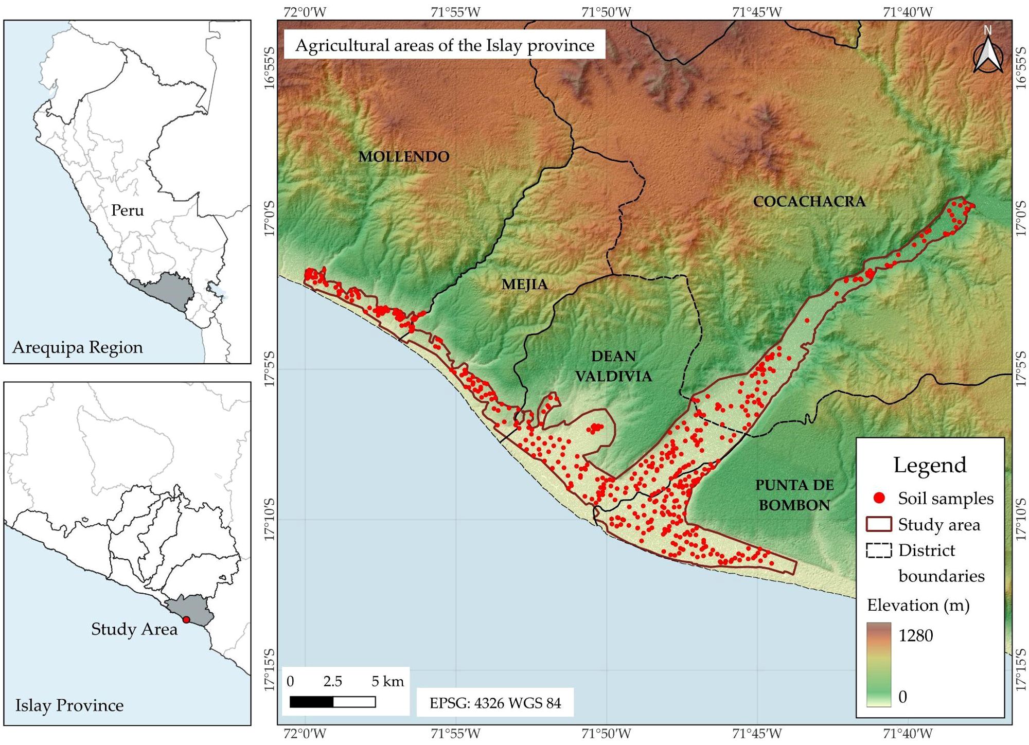
Figure 1. Location of the 491 soil samples in the districts of Cocachacra, Deán Valdivia, Mejía, Mollendo, and Punta de Bombón, province of Islay, Arequipa.

2.2 Soil sampling

Soil sampling followed the methodology described by Havlin et al. (36), in which each sample is assigned to a homogeneous agricultural unit (HAU). HAUs were delineated according to slope class (hillside vs. flat areas), soil texture and color, crop species and varieties, and a maximum unit size of 10 ha. Within each HAU, ten subsamples were randomly collected from each plot at a depth of 0–30 cm, yielding approximately 1 kg of composite soil per unit. Samples were placed in waterproof polyethylene bags, clearly labeled, and stored under cool conditions to minimize changes in physical and chemical properties. The geographic coordinates of each sampling location were recorded using a GPS device. In total, 491 composite soil samples were collected from agricultural fields representing different cropping systems in the province of Islay, Arequipa, Peru.

2.3 Soil analysis

Soil samples were pretreated following ISO 11464:2006 (37), by air-drying at < 40°C and sieving to obtain the fine fraction (< 2 mm) prior to physical and chemical analyses at the INIA laboratory. Soil texture was determined using the Bouyoucos hydrometer method (AS-09), pH was measured in a 1:1 soil-to-water suspension (38, 39), and electrical conductivity in a 1:5 extract (40). Organic matter content was determined by the Walkley–Black oxidation method, available phosphorus (Pav) by the Olsen method, available potassium (Kav) by extraction with ammonium acetate, and total nitrogen by the modified Kjeldahl method (41). Total concentrations of Cu, Fe, Pb, Zn, As, Ba, Al, Mn, Cd, Sr, and Cr were measured using microwave-assisted acid digestion followed by inductively coupled plasma atomic emission spectroscopy (ICP-AES), in accordance with SEMARNAT (42) and US EPA methods 3051A (43), 6010B (38), 6010C (44), and 6010D (45). Since this method is not intended to accomplish total decomposition of the sample, the extracted analyte concentrations may not reflect the total content in the sample (43).

2.4 Extraction and processing of geospatial variables

Geospatial layers compatible with the regional scale were integrated to characterize factors influencing soil property distribution. The geomorphology layer was obtained from the 1:250–000 national geomorphological map (46, 47), enabling the identification of major landform units associated with accumulation and runoff processes. Parent material and geological age were derived from the 1:100–000 national geological map, providing lithological detail to differentiate relevant rock formations. The life zone classification (48) at 1:100–000 scale incorporated ecological factors such as climate and altitude, while climate classification from IDESEP (11) at 1:400–000 scale provided a macro-level view of the climatic environment. Slope was derived from 30 m Shuttle Radar Topography Mission (SRTM) data (49) to improve relief interpretation, and mean temperature and precipitation for February–May were extracted from the WorldClim 2.1 dataset at 30-arc-second resolution (~ 1 km) (35).

Soil type, bulk density (BD), and cation exchange capacity (CEC) were obtained from the SoilGrids 2.0 database (50) at 250 m spatial resolution. For BD and CEC, values from the 0–15 cm and 15–30 cm depth layers were averaged to represent the topsoil zone sampled in the field. Although SoilGrids 2.0 provides advanced global soil predictions, several limitations should be acknowledged. Prediction accuracy varies by property and depth, with higher uncertainty for CEC compared to BD. Additionally, the 250 m resolution may not adequately capture fine-scale spatial heterogeneity or abrupt transitions related to parent material or topography, and model performance is typically lower in data-sparse regions such as the study area, where local training data are scarce.

Normalized Difference Vegetation Index (NDVI) values were derived in Google Earth Engine (GEE) using Sentinel-2 imagery from the COPERNICUS/S2_SR_HARMONIZED collection (51) for February–May in 2021–2024. NDVI was calculated as (B8 – B4)/(B8 + B4), where B8 corresponds to the near-infrared band and B4 to the red band. The district of Islay was delimited using a project vector, and scenes with < 20% cloud cover were selected. Cloud and cirrus masking was applied using the QA60 band, where flagged pixels were excluded from analysis. For each year, a temporal median composite was generated to minimize remaining atmospheric effects and data gaps, NDVI was calculated, and the resulting rasters were clipped to the area of interest. Outputs were visualized in GEE Code Editor using a standardized color palette and exported as GeoTIFF files georeferenced to EPSG:4326, with a spatial resolution of 10 m. The median NDVI across the four-year period (2021–2024) was used to characterize vegetation status at each soil sampling location.

Values from all geospatial layers were extracted at the 491 soil sampling point locations using raster extraction functions in QGIS 3.40.5. Each layer maintained its native spatial resolution during extraction, with pixel or polygon values assigned to points based on spatial overlay. The combination of multi-scale datasets from authoritative sources ensured adequate spatial consistency to identify general soil fertility patterns and their environmental drivers.

2.5 Univariate statistical analysis

Univariate descriptive analysis was conducted in R v4.4.1 (52). Data were imported using the read.delim function, and numerical variables were automatically selected with the dplyr package. Subsequently, key descriptive statistics were computed, including mean, standard deviation, variance, coefficient of variation, skewness, kurtosis, minimum and maximum values, 25th and 75th percentiles, median, and the p-value of the Shapiro–Wilk normality test. Finally, the results were arranged in both long and wide formats using the tidyr package, enhancing their clarity and facilitating interpretation.

2.6 Multivariate statistical analysis

The relationships among numerical variables were examined using Spearman’s rank correlation coefficient, calculated with the rcorr function from the Hmisc package. This procedure generated correlation and p-value matrices, from which only statistically significant coefficients (p < 0.01) were visualized using the corrplot package.

To reduce dimensionality and identify multivariate patterns, Principal Component Analysis (PCA) was conducted with FactoMineR and visualized with factoextra. Variable selection for PCA was based on Spearman correlation with NDVI, including only variables with |r| > 0.30 and p < 0.01 to focus on the factors most relevant to vegetation dynamics. Selected variables were standardized prior to analysis, and categorical variables were excluded. Qualitative factors were coded as factor variables to distinguish clusters in the biplots. The eigenvalues, variable contributions, quality of representation (cos²), and the distribution of samples in the factorial space were examined, with confidence ellipses included. All graphical representations were created using ggplot2.

2.7 Calculation of the weighted soil fertility index

The analysis began with a minimum data set comprising eight edaphic and vegetation indicators, selected based on Spearman’s rank correlation coefficient. After standardizing the variables, Principal Component Analysis (PCA) was conducted using the PCA function from the FactoMineR package, retaining as many components as required to explain at least 70% of the total variance. Variable contributions to these components, together with the explained variances, were used to derive specific weights ($W_i$), from which a weighting matrix was generated via matrix multiplication. Each indicator was then normalized using linear scoring functions according to predefined thresholds and “more is better” or “less is better” criteria, using Equations 1 and 2:

$\begin{array}{ll}M(x)=\{\begin{array}{c}0.1 , x\le x_1\\ 0.1+0.9\left(\frac{x-x_1}{x_2-x_1}\right), x_1\le x\le x_2\\ 1 , x\ge x_2\end{array}& (1)\end{array}$

$\begin{array}{ll}L(x)=\{\begin{array}{c}1 , x\le x_1\\ 1-0.9\left(\frac{x-x_1}{x_2-x_1}\right), x_1\le x\le x_2\\ 0.1 , x\ge x_2\end{array}& (2)\end{array}$

where $M(x)$ and $L(x)$are functions of ‘more is better’ and ‘less is better’, respectively, with values restricted between 0.1 and 1.0. These values represent the lowest (0.1) and highest (1.0) possible scores. $x$ represents the measured value of the indicator, while $x_1$ and $x_2$ are the threshold values (inflection points) for the function curve.

The Weighted Soil Fertility Index (SFIw) was computed as the sum of each normalized score multiplied by its corresponding weight, and subsequently classified into Low, Medium, and High categories using tertiles. The equations for the weighted coefficients (Equation 3) and the fertility index (Equation 4) are as follows:

$\begin{array}{ll}{W}_i=\frac{{\sum }_{j=1}^p(C_{ij}\times V_j)}{{\sum }_{j=1}^p{V}_j}& (3)\end{array}$

where $C_{ij}$ is the contribution of variable i in component j, and V_j is the proportion of variance explained by component j.

$\begin{array}{ll}SF{I}_w={\displaystyle \sum _{i=1}^n{W}_i{N}_i}& (4)\end{array}$

where $N_i$ corresponds to the normalized (0–1) value of each variable, and $W_i$ to its relative weight. The final SFIw value ranges from 0 to 1. All data processing and calculations were performed within the tidyverse environment in R.

2.8 Non-parametric comparison analysis

To compare soil properties among groups defined by district, parent material, and geological age, non-parametric tests were applied, as the data did not meet the assumptions of normality or homogeneity of variances. The Kruskal–Wallis test was first used to detect overall differences in median values for each variable. When significant effects were observed (p < 0.05), pairwise multiple comparisons were conducted using Dunn’s test with Bonferroni adjustment, implemented via the dunnTest function in the FSA package. Factor levels were assigned letters based on adjusted p-values, using the multcompLetters function from the multcompView package. These groupings facilitated the identification of significantly different pairs. Finally, variable distributions were visualized as boxplots with overlaid jittered points using ggplot2.

2.9 Regression kriging

Regression kriging (RK) combines a deterministic trend $m(S_0)$ with a spatially correlated stochastic residual $e(S_0)$, so that the prediction at location $S_0$ is expressed as follows (Equation 5):

$\begin{array}{ll}Z(S_0)=m(S_0) + e(S_0)={\displaystyle \sum _{k=i}^p{\beta }_k}·q_k(S_0)+{\displaystyle \sum _{i=1}^N{\lambda }_i}·e(S_i) & (5)\end{array}$

where ${\beta }_k$ are the regression coefficients associated with $p$ covariates $q_k$, ${\lambda }_i$ are the kriging weights, $N$ is the number of observations and $e(S_i)$ regression residues at each point $S_i$ (53). The spatial dependency structure of these residues is characterized using the semivariogram (Equation 6):

$\begin{array}{ll}\gamma (h) = \frac{1}{2}E[{z(x)-z(x+h)]}^2 & (6)\end{array}$

where E represents the variance, and $z(x)$ and $z(x+h)$ are paired values separated by the distance $h$ (54). In practice, regression is first fitted using environmental covariates derived from remote sensing, geological, and land-use maps. The residuals from this model are then interpolated using kriging, and the sum of the regression predictions and kriged residuals constitutes the final map of the target variable (55, 56).

For the implementation of this model, SAGA GIS v9.7.1 was used to spatially model the Weighted Soil Fertility Index (SFIw). The covariates selected for the regression component were soil type (TS), geoform (GM), and normalized difference vegetation index (NDVI). Empirical evidence from case studies has shown a strong association between these variables and soil fertility variability. Previous research has demonstrated that landform attributes influence the relationship between soil properties and physiographic factors such as relief, slope, and altitude, thereby affecting soil fertility patterns (57, 58). Similarly, soil type integrates key edaphic properties such as texture, mineralogy, and drainage, which control nutrient-retention capacity and overall fertility potential (59). In turn, NDVI has been widely used as a biophysical indicator of vegetation vigor and health (60).

2.10 Validation of the regression kriging model

The selection of the semivariogram model in the geostatistical analysis was based on evaluation criteria such as the coefficient of determination (R²) (Equation 7), root mean square error (RMSE) (Equation 8), and mean absolute error (MAE) (Equation 9). The optimal model was defined as that with RMSE values close to zero and R² values close to one. The formulas used to calculate these evaluation indices are as follows:

$\begin{array}{ll}{R}^2 =1 -\frac{{\sum }_{I = 1}^n{[Z_1(x_i)-Z_2(x_i)]}^2}{{\sum }_{I = 1}^n{[Z_1(x_i)-Z_1]}^2} & (7)\end{array}$

$\begin{array}{ll}RMSE = \sqrt{\frac{1}{n}{\displaystyle \sum _{i=1}^n{[Z_1(x_i)-Z_2(x_i)]}^2}}& (8)\end{array}$

$\begin{array}{ll}MAE =\frac{1}{n}{\displaystyle \sum _{i=1}^n|Z_1(x_i)-Z_2(x_i)|}& (9)\end{array}$

Validation of the regression kriging interpolations was performed using leave-one-out cross-validation (LOOCV), an iterative process in which, at each step, one observation is omitted and its value predicted using the model fitted to the remaining data. This procedure yields a set of residuals calculated as the difference between observed and predicted values; these residuals are then analyzed to infer their distribution and assess model performance (61). Although this approach is computationally demanding, it provides an error estimate that closely approximates maximum likelihood (62).

3 Results

3.1 Spearman’s rank correlation between edaphoclimatic variables and the spectral vegetation vigor index

Spearman’s rank correlation analysis was used to evaluate non-parametric monotonic associations between 22 physicochemical soil properties, slope, mean temperature (Tmean), and mean monthly precipitation (Pmon) and the spectral index of vegetative vigor (NDVI) (Figure 2). This analysis revealed potential patterns of covariance between NDVI and edaphic factors related to processes such as sandy soil alkalinity, phosphorus and micronutrient availability, chromium toxicity, and soil compaction.

Figure 2

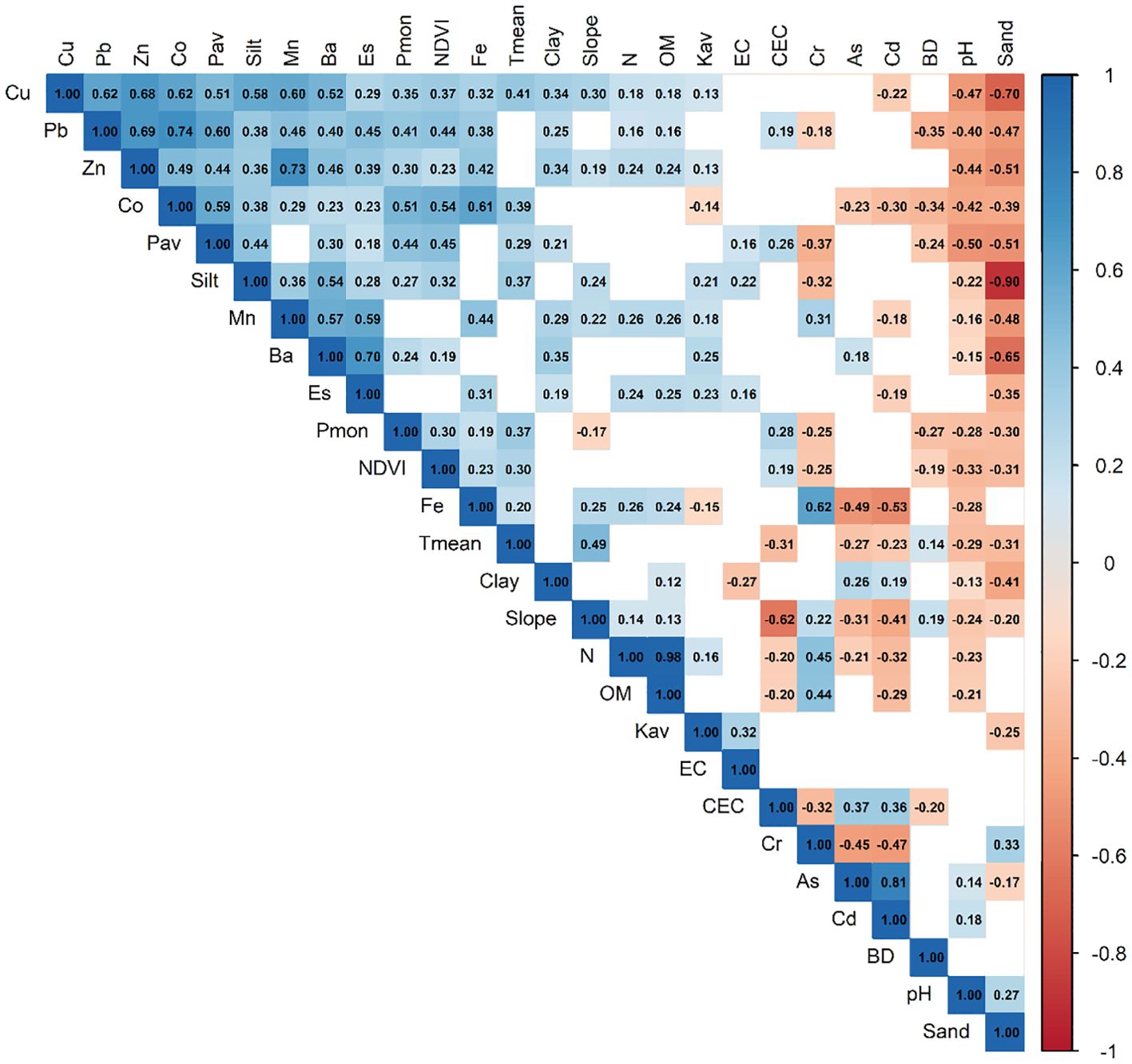
Figure 2. Spearman’s non-parametric bivariate correlation matrix between NDVI, 22 physicochemical soil properties, slope, mean temperature (Tmean), and mean monthly precipitation (Pmon). Only statistically significant correlations (p < 0.01) are displayed; blank cells indicate non-significant relationships. CEC, cation exchange capacity; BD, bulk density.

Moderate positive correlations (r > 0.30) were observed between NDVI and total Co (0.54), Pav (0.45), total Cu (0.37), silt percentage (0.32), Tmean (0.30), and Pmon (0.30). Conversely, moderate negative correlations (r < −0.30) were found with pH (−0.33) and sand percentage (−0.31).

3.2 Statistical distribution of soil properties most influencing vegetation health

Table 1 presents the descriptive statistics for 12 physicochemical soil properties associated with NDVI variability, based on 491 samples collected from diverse agricultural systems in the province of Islay. NDVI values ranged from 0.03 to 0.86, with a mean of 0.58 and a coefficient of variation (CV) of 33.67%, indicating moderate spatial variability in vegetation vigor. The distribution was slightly skewed toward higher values and exhibited near-normal kurtosis, reflecting a predominance of medium-to-high values and few extremes.

Table 1

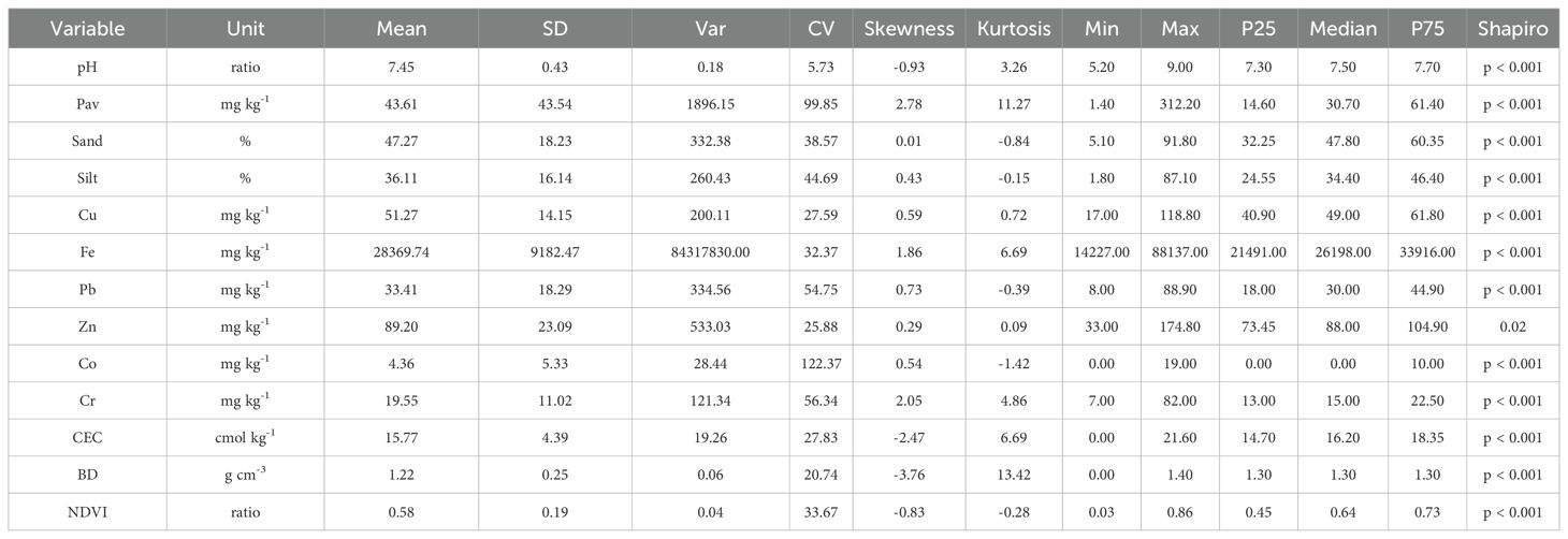
Table 1. Descriptive statistics of 12 soil physicochemical parameters significantly correlated with NDVI in the province of Islay.

Soil pH averaged 7.45, close to neutral, with low dispersion (CV = 5.73%), although slightly skewed toward alkaline conditions. In contrast, Pav showed very high variability (CV = 99.85%) and a strongly skewed, leptokurtic distribution. Approximately 25% of the samples had values below 14.60 mg kg^-¹, while localized areas exhibited high concentrations, likely associated with heterogeneous fertilization practices.

Textural fractions exhibited contrasting patterns: sand content had a symmetrical but widely dispersed distribution (CV = 38.57%), silt content was more variable (CV = 44.69%) and slightly skewed toward lower values, suggesting notable differences in soil physical structure.

Micronutrients also showed considerable variability. Iron (Fe) had a high mean and was skewed toward higher values, with markedly leptokurtic kurtosis, indicating the presence of soils with substantial Fe accumulation. Zinc (Zn) and copper (Cu) displayed lower dispersion but were also skewed toward high concentrations. Cobalt (Co) exhibited extreme skewness, with most values near zero but a few very high outliers.

Finally, cation exchange capacity (CEC) and bulk density (BD) showed opposite tendencies: CEC displayed moderate variability with slight negative skewness, reflecting differences in nutrient retention capacity, whereas BD exhibited a highly leptokurtic distribution with strong negative skewness, indicating a predominance of loose, low-compaction soils. Overall, these statistical patterns reveal pronounced heterogeneity in the edaphic properties that directly influence crop performance and productivity in the province of Islay.

3.3 Edaphic gradients associated with vegetation vigor revealed by principal component analysis

Principal component analysis (PCA) was performed using the variables most strongly correlated with NDVI, after reducing collinearity and transforming them to homogenize variances. The first and second principal components together explained 60.47% of the total variance (Table 2).

Table 2

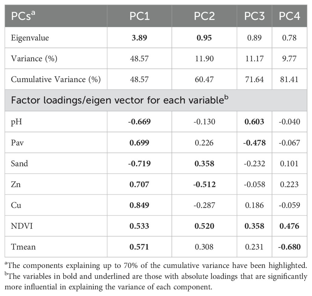
Table 2. Results of the principal components analysis (PCA) for soil properties in the study area.

The first principal component (PC1, 48.57% of variance) was characterized by high positive loadings for Cu (0.85), Co (0.78), Zn (0.71), and Pav (0.70), and strong negative loadings for sand content (–0.72) and pH (–0.67). This axis represents a fertility–texture gradient, ranging from soils enriched in essential micronutrients and phosphorus, with higher NDVI and moderate texture, to sandy, alkaline soils with low nutrient- and water-retention capacity.

The second principal component (PC2, 11.90% of variance) was positively associated with NDVI (0.52), sand content (0.36), and mean temperature (0.31), and negatively with Zn (–0.51) and Cu (–0.29). This axis represents a thermal–vigor gradient coupled with a textural–micronutrient trade-off, where higher NDVI and temperature are associated with sandier soils and reduced Zn and Cu contents. This pattern suggests that increasing sand content is linked to lower micronutrient availability—particularly Zn—likely due to leaching and limited cation retention in coarse-textured soils. Such conditions may enhance vegetation vigor under favorable moisture and temperature regimes but constrain nutrient accumulation, consistent with nutrient dilution or localized management effects influencing plant performance.

The PC1–PC2 biplot (Figure 3) reveals clear edaphic differentiation among the agricultural districts of Islay Province. Cocachacra clusters on the positive side of PC1, associated with higher Co, Cu, and Pav levels, elevated NDVI, and lower pH—conditions indicative of fertile, moderately textured soils that favor nutrient availability and vigorous vegetation growth. Deán Valdivia also occupies the positive domain of PC1 but exhibits moderate dispersion along PC2, reflecting slight variation in temperature and NDVI among sites.

Figure 3

Figure 3. Principal component analysis (PCA) of edaphic variables showing the regional multivariate distribution along Dimension 1 (Dim1, ~48.6%) and Dimension 2 (Dim2, ~11.9%), with 44% confidence ellipses.

In contrast, Mejía and Mollendo are positioned on the negative side of PC1, where high sand content and elevated pH dominate. These conditions correspond to coarser, alkaline soils with reduced water-holding capacity, lower aggregate stability, and limited micronutrient and phosphorus availability. Consequently, management strategies in these districts should emphasize soil structure improvement and phosphorus supplementation.

Punta de Bombón spans a wide area across both axes, denoting marked internal heterogeneity. Some sites approach the central region of the plot, whereas others extend toward the negative extremes of PC1, reflecting sandy, Zn- and Cu-deficient soils consistent with the low NDVI observed in this district. This pronounced edaphic variability highlights the need for detailed soil zoning and targeted fertilization practices to optimize nutrient use efficiency and vegetation vigor.

3.4 Non-parametric comparison of the weighted soil fertility index among districts, soil taxonomic types (WRB), and parent material in Islay Province

The Kruskal–Wallis test indicated significant overall differences in SFIw among districts (p < 0.001; Figure 4a). Post hoc Dunn’s tests showed that soils in Cocachacra (median = 0.60) and Deán Valdivia (0.50) exhibited significantly higher SFIw values than those in Mejía (0.20), Mollendo (0.20), and Punta de Bombón (0.30). These patterns indicate that soils in Mollendo, in particular, have the lowest NDVI values and are characterized by alkalinity with low available Co, Cu, Zn, and P.

Figure 4

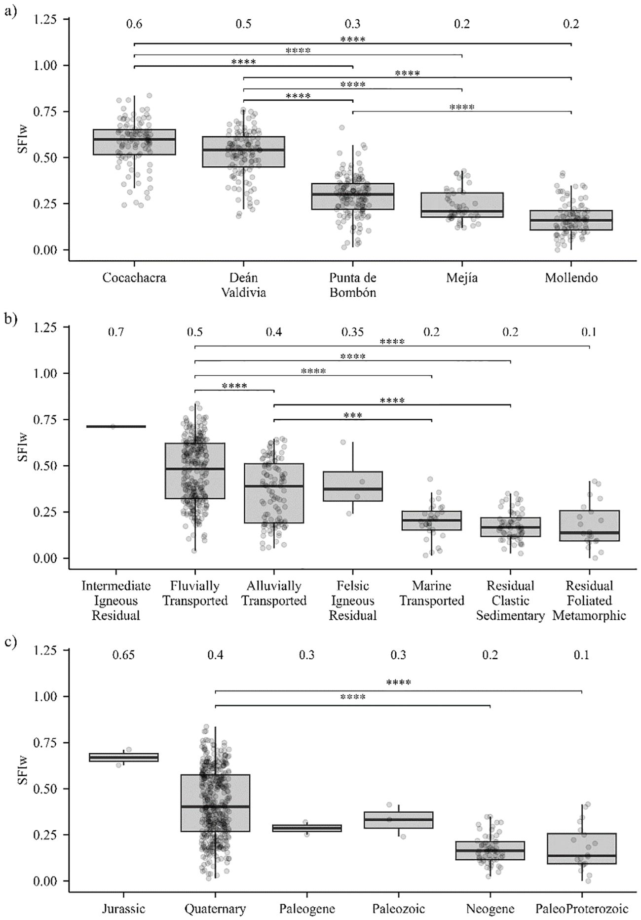
Figure 4. Weighted soil fertility index (SFIw) based on different factors: (a) comparison among districts in the province of Islay, (b) comparison among parent material types, and (c) comparison among geological ages of parent material. The Dunn post hoc test was performed following the Kruskal–Wallis test, with Bonferroni correction for multiple comparisons. Different letters indicate statistically significant differences. Statistical differences are shown as “***” for p-adj < 0.001 and “****” for p-adj < 0.0001.

Regarding parent material, highly significant differences in SFIw were detected (p-adj < 0.001; Figure 4b). Soils developed from fluvial and alluvial deposits had the highest SFIw medians (0.50 and 0.40, respectively), exceeding those of soils derived from marine-transported, clastic sedimentary residual, and foliated metamorphic residual materials (0.20, 0.20, and 0.10, respectively).

Differences were also significant according to geological age (p-adj < 0.001; Figure 4c). Soils with Quaternary parent materials presented the highest SFIw values (0.40), surpassing those developed from Paleoproterozoic and Neogene substrates (0.10 and 0.20, respectively).

Overall, these results highlight the influence of lithological origin on current soil quality and can inform the development of targeted fertility management strategies based on parent material in heterogeneous arid landscapes.

3.5 Spatial variation of the weighted soil fertility index in the province of Islay

In the province of Islay, a continuous map of the SFIw was generated using a regression kriging model. Prior analysis (Correlation and PCA) had identified pH, Pav, Zn, Co, Cu, sand content, and NDVI as important variables driving soil fertility (Figure 5). For the spatial modeling, geomorphology, soil type, and NDVI were selected as the optimal set of three spatial predictors. A multiple regression model using these three predictors was constructed to capture the deterministic trend of the SFIw. Ordinary kriging was then applied to the model residuals to capture the remaining spatial stochastic spatial structure. This combined regression–kriging approach yielded high-resolution and robust predictions of SFIw across the province (Figure 6), establishing a clear basis for designing site-specific management and fertilization strategies.

Figure 5

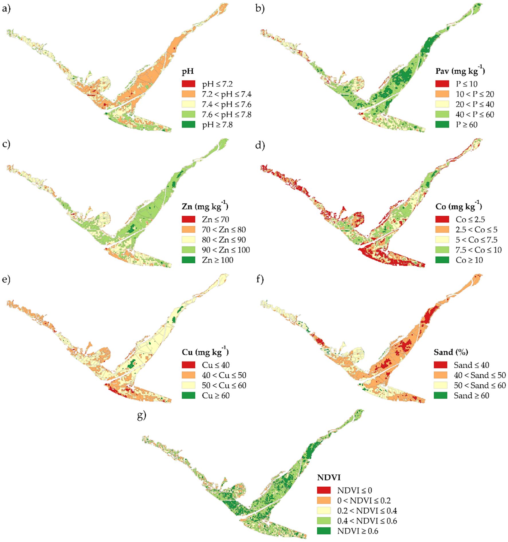
Figure 5. Spatial distribution of selected predictors in the province of Islay: (a) pH, (b) available phosphorus (Pav), (c) zinc, (d) cobalt, (e) copper, (f) sand content, and (g) normalized difference vegetation index (NDVI).

Figure 6

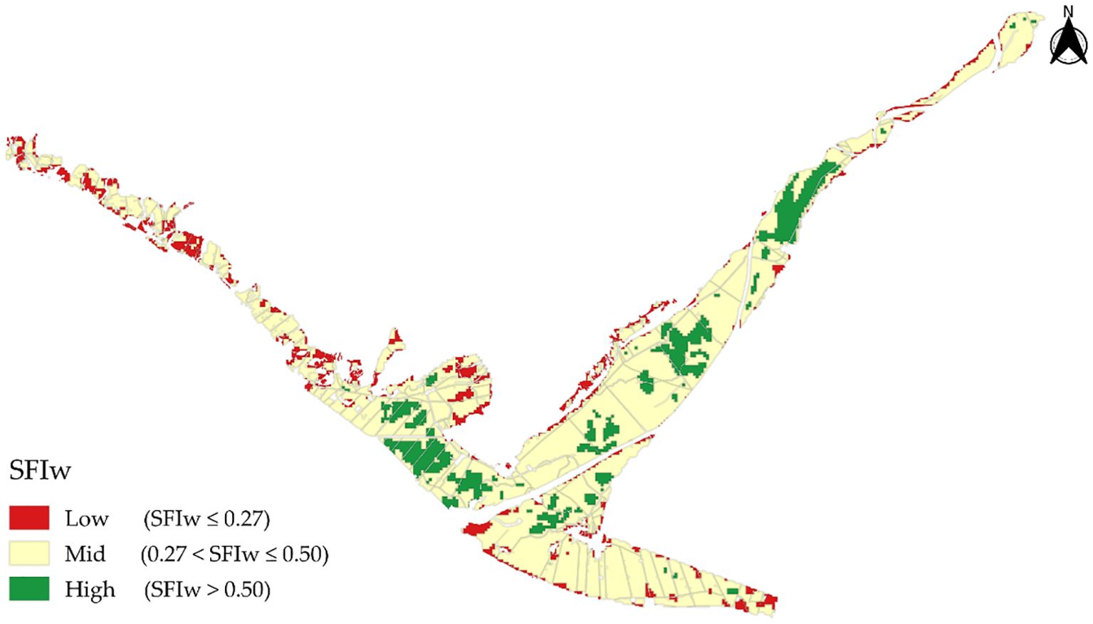
Figure 6. Spatial distribution of the SFIw in agricultural areas of the province of Islay, classified into low, medium, and high.

Table 3 details the parameters of the semivariogram models obtained using the regression kriging (RK) interpolation method, along with the results of cross-validation based on RMSE, MAE, and R². The semivariogram fitted with the Exponential model was the most suitable for predicting the spatial variability of SFIw, yielding a satisfactory prediction (R² = 0.68, RMSE = 0.11, MAE = 0.09).

Table 3

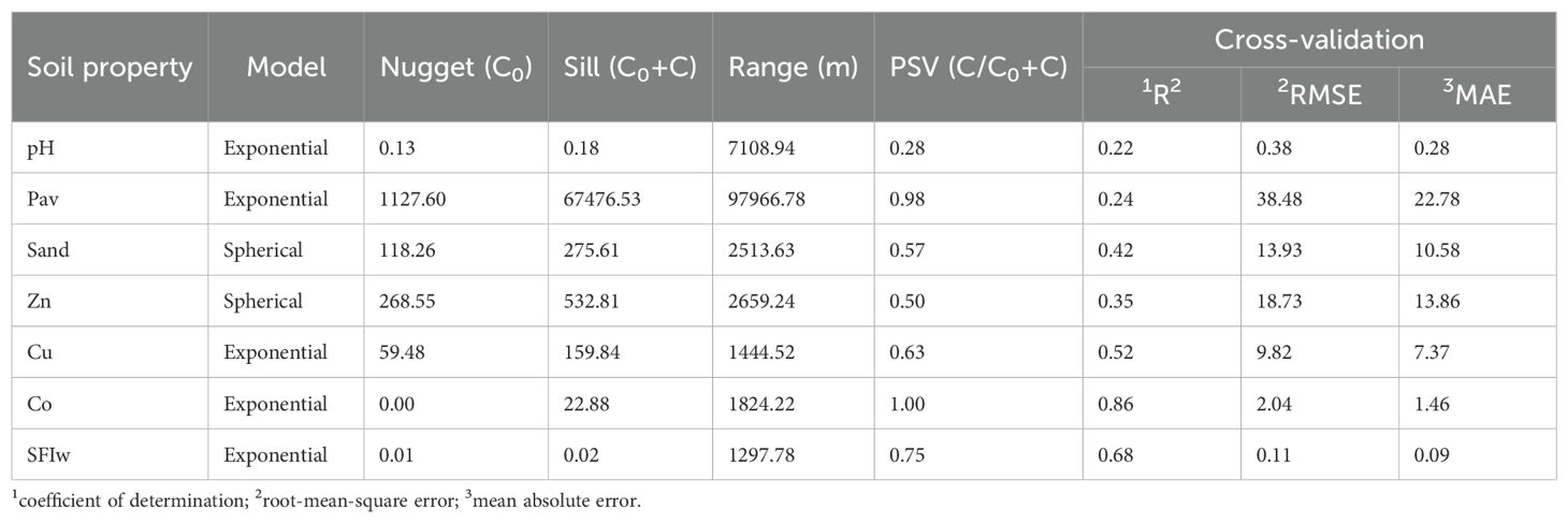
Table 3. Semivariogram parameters and cross-validation for the regression kriging models.

Within the study site, the classified agricultural areas totaled 9272.62 ha. The Medium class was predominant for SFIw, covering 76.4% of the total (7085.21 ha), followed by the High class with 13.3% (1232.11 ha) and the Low class representing 10.3% (955.3 ha) (Table 4). Figure 6 shows the spatial distribution of SFIw for the agricultural areas according to this classification.

Table 4

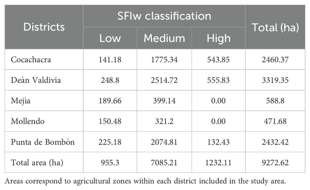
Table 4. Area distribution (ha) of SFIw fertility classes by district.

4 Discussions

4.1 Edaphic determinants of vegetation vigor: correlation analysis between NDVI and soil properties

The results reveal significant correlations between NDVI and the main soil indicators (physical, chemical, and mineralogical soil variables). The moderate positive correlation of NDVI with available phosphorus (Pav) and total Cu, Co, and Zn is consistent with the scientific literature, considering that Cu and Zn are essential micronutrients, P is a critical macronutrient, and Co, although not essential, is regarded as a beneficial element for plants (36).

Copper (Cu) plays a fundamental role in photosynthesis as a component of plastocyanin, an electron-transport protein in Photosystem I (63). In addition, this element is involved in key processes such as mitochondrial respiration and nitrogen metabolism (63, 64). Under Cu deficiency, typical symptoms include interveinal chlorosis, resulting from reduced photosynthetic efficiency and decreased carbohydrate production during the vegetative phase (63). Zinc (Zn) participates in multiple physiological processes in plants, including chlorophyll synthesis, enzymatic activation, and the preservation of cell membrane integrity (63). Its deficiency typically manifests in young leaves as interveinal chlorosis, which can negatively affect photosynthesis (36) and, consequently, reduce NDVI values.

Phosphorus (P) is a structural component of phospholipids, phosphoproteins, enzymes, DNA, RNA, ADP, and ATP (65). The latter two are involved in multiple processes such as photosynthesis and cellular respiration (36). Furthermore, P is associated with increased root growth, which indirectly enhances parameters such as leaf area index and photosynthetic rate (66).

Cobalt (Co), although not considered an essential element, can improve photosynthetic efficiency by delaying leaf senescence and reducing ethylene production, thereby maintaining the functionality of the photosynthetic apparatus for longer periods (67, 68). Additionally, Co acts as a component of cobalamin, which is required by symbiotic, endophytic, and associative bacteria involved in biological nitrogen fixation (69). This process contributes significantly to the productivity of major crops such as beans, soybeans, rice, corn, barley, wheat, and sugarcane (69), suggesting that the observed relationship between soil Co content and NDVI may reflect enhanced microbial activity and nitrogen availability that promote plant growth and canopy vigor in our study area.

Therefore, the positive correlation between these elements and NDVI can be explained by their direct or indirect involvement in photosynthetic processes that determine vegetation density and vigor, traits quantified by NDVI through reflectance in the red and near-infrared bands. NDVI can thus be used as an indirect indicator of soil fertility to support precision agriculture; however, its interpretation must consider the environmental context, especially in arid and semiarid regions where vegetation can be strongly affected by water availability. Although NDVI generally reflects vegetation vigor and nutrient status, under water-limited conditions its response can be constrained by soil moisture rather than nutrient supply (70, 71). Periodic drought stress reduces stomatal conductance and photosynthetic rate, thereby limiting canopy development and greenness even in relatively fertile soils (72). Conversely, areas with finer textures and higher organic matter tend to retain more water, buffering the effects of drought and enhancing nutrient diffusion and root uptake (73). Thus, in arid systems, positive correlations between NDVI and fertility indicators reflect not only nutrient sufficiency but also improved soil physical conditions that support better water retention and root growth. In contrast, some soil attributes exhibited negative correlations with NDVI, reflecting edaphic constraints on nutrient availability.

The negative correlation observed between NDVI and both soil pH and sand content can be attributed to the limitations these factors impose on nutrient availability. Soil pH regulates the solubility and availability of essential nutrients; under slightly acidic to neutral conditions (pH 5.5–7.0), these elements exhibit greater solubility and accessibility to plants. In contrast, high pH values and elevated CaCO₃ content in alkaline soils often induce deficiencies of essential micronutrients, particularly Fe and Zn, as well as macronutrients such as P, thereby constraining plant nutrition and development (74). Sandy soils, characterized by a low clay fraction, have limited nutrient retention capacity and, due to their high proportion of macropores, exhibit reduced water-holding capacity (75).

4.2 Identification of management zones based on SFIw: variability among districts, parent material, and geological age

Arid and semiarid regions exhibit extreme variations in soil fertility parameters, such as low organic matter content, high phosphorus fixation, elevated pH, salinity and alkalinity, together with the presence of carbonates and gypsum (14, 76). These characteristics make fertility indices developed for humid regions unsuitable when applied to these dryland environments. To overcome this limitation, a Soil Fertility Index for water-limited regions (SFIw) is established through principal component analysis (PCA), which identifies the most influential edaphic variables (14).

The integration of the Soil Fertility Index for water-limited regions (SFIw) into agronomic interpretation enables the classification of soil fertility into three ranges based on tertile-derived thresholds. The low index (SFIw ≤ 0.26) indicates severe limitations in nutrient availability and physical properties (e.g., high sand content, elevated pH), which require intensive replenishment strategies (77) and are often associated with low fruit yields (78). The medium index (0.27 ≤ SFIw ≤ 0.50) reflects moderate fertility, suitable for maintenance management in which nutrient inputs are adjusted to crop extraction to preserve critical nutrient thresholds. Finally, the high index (SFIw > 0.50) denotes good soil structure, high nutrient retention, and optimal fertility levels. In semi-organic rice systems, SFIw values above 0.75 have been reported, associated with high productivity and profitability (79). This classification is essential for guiding site-specific management practices that promote both environmental and economic sustainability.

The spatial distribution of SFIw across the study area revealed marked variability both among and within districts. Soils in Cocachacra and Deán Valdivia exhibited the highest SFIw values, followed by Punta de Bombón with moderate values, whereas Mejía and Mollendo showed the lowest levels. This heterogeneity can be mainly attributed to differences in parent material and the geological age of the deposits (Figures 5 and 6).

Parent material can be a decisive factor in current soil fertility since it provides most of the nutrients required by plants, except for oxygen, hydrogen, nitrogen, and carbon, which are derived from the atmosphere and organic matter (80).

In this study, soils formed on fluvial and alluvial materials showed higher SFIw values than those developed on marine-transported, clastic sedimentary, and foliated metamorphic substrates.

The superiority of SFIw observed in materials transported from fluvial and alluvial sources could be explained by the fact that deposits in floodplains (“fluvial fans”) tend to be enriched in nutrients, which makes them highly fertile and productive. This phenomenon is attributable to the continuous influx of sediments resulting from soil erosion in higher regions. Alluvial deposits, comprising detrital materials, frequently exhibit substantial agricultural productivity. However, these deposits often possess relatively coarse textures, which can influence their physical properties, such as water and nutrient retention (74).

In contrast, marine parent materials exhibit variability in soil texture, ranging from sandy to clayey (74). In the present study, the soils derived from marine deposits are likely to correspond to sandy materials. According to Gray and Murphy (81), sandy marine deposits are predominantly composed of quartz sands (SiO₂), which typically display low CEC and fertility.

Similarly, residual clastic sediments show variability in texture and composition. These represent the remnants of rocks that could not be dissolved during weathering processes and are generally composed of minerals highly resistant to chemical alteration (quartz and silicate minerals) or of neoformation minerals, particularly clay minerals and aluminum hydroxides (82). A portion of the soils examined in this study developed on this parent material, and they likely exhibited low fertility due to the predominance of quartz in their mineralogical composition, a chemically inert mineral that limits nutrient availability.

The geological age of the parent material also influenced SFIw. Soils developed on recent deposits (Quaternary) exhibited the highest SFIw values, in contrast to those formed on older deposits (Neogene and Paleoproterozoic).

The Quaternary period, spanning the last 2.6 million years, is characterized by a climate strongly influenced by glaciations. During this period, a wide range of sedimentary deposits originated, including alluvial, fluvial, marine, glacial, periglacial, and aeolian deposits (83). In the present study, the higher fertility observed in Quaternary soils may be attributed to the fact that much of the agricultural land in the province of Islay developed on alluvial and fluvial sediments.

The Neogene (23–2.6 Ma), preceding the Quaternary, was characterized by a climate that was initially temperate, followed by a progressive cooling trend. Intense tectonic activity promoted erosion and the accumulation of detrital sediments, along with volcanic and marine–continental deposits associated with sea-level fluctuations (84). The relatively low fertility (SFIw) observed in soils derived from this period may be attributed to their development on residual clastic sediments, which are characterized by high resistance to weathering.

The Paleoproterozoic Era (2420–1780 Ma) was characterized by global glaciations, a significant increase in atmospheric oxygen, and the reappearance of banded iron formations (BIF) (85). During this period, parent material consisted of strongly weathered, acidic, and highly oxidized rocks, conditions that promoted intense phosphorus mobilization and loss as a consequence of rising atmospheric oxygen and the oxidation of minerals such as pyrite (86). This early depletion of phosphorus in parent material could explain the low SFIw values observed in soils derived from this geological era.

4.3 Fertilization and edaphic correction strategies based on the spatial variability of soil fertility in the Tambo Valley

The results discussed in Section 4.2 demonstrate that soil fertility is strongly influenced by parent material, with fluvial soils emerging as the most fertile, followed by alluvial soils. Cocachacra and Deán Valdivia exhibited significantly high SFIw values of 0.60 and 0.50, respectively, whereas soils developed on marine deposits, residual clastic sedimentary materials, and foliated metamorphic substrates showed lower fertility, as observed in Mejía (0.20), Mollendo (0.20), and Punta de Bombón (0.30). This pattern is consistent with recent studies reporting higher phosphorus availability and greater retention capacity in fluvial sediments compared to clayey or residual soils (87, 88). The marked spatial heterogeneity observed (see Figure 6) reinforces the need to adopt site-specific management strategies, in line with modern principles of precision agriculture and variable-rate fertilization (89).

The NDVI showed significant correlations: a positive relationship with available phosphorus and a negative relationship with pH and sand content, indicating that fertilization recommendations must be adapted to local edaphic conditions. In this context, phosphorus fertilization should be guided by the soil P level relative to the critical level (CL), following three approaches: (i) the build-up or sufficiency strategy, which applies rates greater than crop removal to raise soil P above limiting levels when values fall below the CL; (ii) the maintenance strategy, in which applications are adjusted to replace only the amount removed by the crop when soil P is close to or slightly above the CL; and (iii) the suspension of fertilization in soils with P levels above the CL, accompanied by annual monitoring (36, 90).

According to the results presented in Figure 5, the districts of Cocachacra, Deán Valdivia, and Punta de Bombón exhibit high levels of available phosphorus and therefore, in general, require maintenance fertilization. In contrast, in the districts of Mejía and Mollendo, where variable phosphorus levels (low, medium, and high) were identified, enrichment and maintenance strategies are recommended. Since no previous studies in the study area have established a crop-specific critical level (CL), phosphorus fertilization recommendations were based on the nutrient balance method (91, 92), considering the total crop P₂O₅ extraction (4.42 kg ha^-¹; 93), which allows for estimating MAP doses adapted to local variability. By integrating fertility indices (low, medium, high) with interquartile ranges (25th–75th percentiles) of available phosphorus, a dosing scheme more representative than conventional averages was obtained (Table A1).

In the low fertility index category, phosphorus requirements exceeded 567 kg ha^-¹ of monoammonium phosphate (MAP), reflecting a low availability of phosphorus. This highlights the importance of splitting fertilizer applications to improve nutrient use efficiency and reduce losses by immobilization or leaching, as previously demonstrated in minimum tillage systems and under high spatial variability of P (88, 94). For the medium index, the wide range observed between quartiles suggests that using an average dose may be insufficient in many cases; therefore, adjustments should be made according to the specific field location (15). In soils classified with a high fertility index, it has been shown that moderate fertilization allows for reaching optimal phosphorus levels without incurring unnecessary costs (88). For these cases, a maximum dose close to 388 kg ha^-¹ is recommended, which can ensure adequate P availability while avoiding the risk of over-fertilization.

This integrative approach, based on fertility indices, enables a more precise calibration of phosphorus fertilization according to edaphic conditions, thereby optimizing fertilizer use and minimizing losses through immobilization or leaching (95). The proposed methodology is of particular relevance for garlic cultivation under the conditions of Arequipa, and its field application could validate and refine these values for highly accurate practical recommendations.

In addition to phosphorus fertilization recommendations, there are environmentally friendly practices that can increase the availability of soil phosphorus. Inoculation of crops with arbuscular mycorrhizal fungi (AMF) can improve phosphorus availability and uptake, thereby reducing or even replacing conventional phosphate fertilization (96). For example, AMF inoculation has been shown to improve garlic yields in soils with moderate P, reducing dependence on phosphate fertilizers (97). Another promising practice is the use of Trichoderma viride as a biofertilizer, since it has demonstrated the ability to solubilize both inorganic and organic insoluble phosphorus while simultaneously stimulating plant growth (98). Furthermore, cover crops represent a promising strategy to improve phosphorus nutrition and crop yields by strengthening plant–microbe interactions and enhancing access to unavailable phosphorus reserves (99).

With regard to soil pH management, soils with values above 7.5 may limit agricultural productivity. To mitigate this alkaline condition, corrective strategies using acidifying organic materials and acid-forming nitrogen fertilization are recommended. For example, in a long-term trial (53 years), ammonium sulfate applied at a rate of 80 kg ha^-¹, together with organic amendments of low calcium content such as peat (3.96 t ha^-¹) and biosolids (6.43 t ha^-¹), proved effective in reducing soil pH, achieving decreases from 6.5 to 4.14, 5.53, and 4.89, respectively (100).

Finally, the sandy soils predominant in the areas of Punta de Bombón, Mejía, and Mollendo could improve their edaphic conditions through the incorporation of acidifying organic materials and the use of cover crops. Beyond the previously described functions, these practices contribute nutrients, enhance microbial activity, improve soil structure and bulk density, increase cation exchange capacity, and reduce water and nutrient losses (74; 101, 102).

Overall, the results emphasize the relevance of coupling soil management practices with spatially explicit diagnostic tools to enhance nutrient efficiency and sustainability. In this context, this study represents the first NDVI-based soil fertility mapping in arid coastal Peru, integrating field soil indicators with remote sensing data through a PCA-weighted index and regression kriging. Beyond its local application, this approach demonstrates how data-driven soil mapping can guide precision agriculture in resource-limited environments (103). By optimizing fertilizer inputs and improving nutrient-use efficiency, the proposed methodology contributes directly to Sustainable Development Goal (SDG) 2 – Zero Hunger, by enhancing agricultural productivity and food security (104, 105), and to SDG 15 – Life on Land, by mitigating soil degradation and promoting sustainable land management (105, 106). In this sense, the integration of soil spatial variability with vegetation indices represents a key strategy for achieving sustainable intensification while minimizing environmental impacts (107).

Furthermore, the observed correlation patterns (e.g., Co–NDVI) open new research avenues into the microbiological and geochemical processes underlying soil fertility in arid systems, linking soil chemistry, microbial activity, and vegetation dynamics (108). Understanding these linkages is essential to maintain soil health and ecosystem services in fragile agroecosystems affected by salinity, alkalinity, and nutrient imbalance—processes that directly threaten both SDG 2 and SDG 15 targets (13, 109).

5 Conclusions

This study successfully integrated soil fertility indicators with NDVI-derived information to develop a weighted Soil Fertility Index (SFIw) for arid coastal agroecosystems in southern Peru. Through PCA-based weighting, Cu, Co, Zn, available phosphorus, sand content, and pH were identified as the most influential soil properties for fertility assessment. The regression kriging model, built upon these indicators and incorporating NDVI, soil type, and geoform data as covariates, achieved satisfactory spatial prediction accuracy (R² = 0.68, RMSE = 0.11).

The high-resolution SFIw map revealed distinct fertility gradients across Islay Province, enabling the delineation of three management zones: (1) High Fertility Maintenance Zone (Cocachacra-Deán Valdivia), requiring balanced nutrient replacement and conservation practices; (2) Medium Fertility Phosphorus Regulation Zone (Punta de Bombón), demanding site-specific P management; and (3) Low Fertility Comprehensive Improvement Zone (Mejía-Mollendo), necessitating integrated soil amendments and pH correction strategies.

Moreover, the integrative approach combining edaphic indicators, spatial modeling, and remote sensing (NDVI) demonstrates strong potential for transferability to other arid and semi-arid regions worldwide, where similar constraints—alkaline pH, nutrient imbalance, and high spatial variability—limit crop productivity. The methodology can thus serve as a replicable framework for regional-scale soil fertility assessment and guiding sustainable land management and precision fertilization strategies under data-scarce conditions.

By linking soil fertility with remotely sensed crop vigor, this research provides a replicable framework for precision agriculture in water-limited environments, supporting both SDG 2 (Zero Hunger) through improved fertilizer-use efficiency and SDG 15 (Life on Land) through soil conservation. To our knowledge, this represents one of the first NDVI-integrated fertility mapping studies in arid coastal Peru. Future research should incorporate multi-temporal NDVI analysis and additional biophysical variables (soil moisture, microbial activity) to better characterize the dynamic interactions between soil fertility, vegetation response, and climate variability in dryland agriculture.

Data availability statement

The raw data supporting the conclusions of this article will be made available by the authors, without undue reservation.

Author contributions

RP: Conceptualization, Investigation, Methodology, Writing – original draft, Writing – review & editing. CV: Formal analysis, Software, Visualization, Writing – original draft. NH: Investigation, Methodology, Writing – original draft. RM: Formal analysis, Investigation, Software, Writing – original draft. SM: Formal analysis, Software, Visualization, Writing – original draft. RR: Investigation, Methodology, Writing – original draft. KQ: Conceptualization, Formal analysis, Supervision, Validation, Writing – review & editing.

Funding

The author(s) declared that financial support was received for this work and/or its publication. The work was funded by the INIA project CUI 2487112 “Mejoramiento de los servicios de investigación y transferencia tecnológica en el manejo y recuperación de suelos agrícolas degradados y aguas para riego en la pequeña y mediana agricultura en los departamentos de Lima, Áncash, San Martín, Cajamarca, Lambayeque, Junín, Ayacucho, Arequipa, Puno y Ucayali”.

Acknowledgments

We also thank the technical staff of the Laboratorio de Suelos, Aguas y Foliares (LABSAF) for carrying out the complete laboratory work, from sample preparation to analysis, and the field teams for their dedicated work during the sampling campaign. Special thanks are extended to the farmers of Cocachacra, Deán Valdivia, Mejía, and Mollendo for granting access to their agricultural fields and sharing valuable agronomic information. During the preparation of this manuscript, the authors used Claude (Claude 3.5 Sonnet, Anthropic) to assist in reviewing English grammar. All generated content was carefully reviewed, edited, and validated by the authors, who take full responsibility for the integrity and accuracy of this publication.

Conflict of interest

The authors declare that the research was conducted in the absence of any commercial or financial relationships that could be construed as a potential conflict of interest.

Generative AI statement

The author(s) declare that no Generative AI was used in the creation of this manuscript.

Any alternative text (alt text) provided alongside figures in this article has been generated by Frontiers with the support of artificial intelligence and reasonable efforts have been made to ensure accuracy, including review by the authors wherever possible. If you identify any issues, please contact us.

Publisher’s note

All claims expressed in this article are solely those of the authors and do not necessarily represent those of their affiliated organizations, or those of the publisher, the editors and the reviewers. Any product that may be evaluated in this article, or claim that may be made by its manufacturer, is not guaranteed or endorsed by the publisher.

Supplementary material

The Supplementary Material for this article can be found online at: https://www.frontiersin.org/articles/10.3389/fsoil.2025.1706974/full#supplementary-material

References

1. Ministerio de Desarrollo Agrario y Riego. Perfil productivo regional - Provincia de Islay [Cuadro de mando interactivo Power BI]. Lima, Peru: Sistema Integrado de Estadísticas Agrarias (SIEA (2025).

Google Scholar

2. Ministerio de Desarrollo Agrario y Riego. Costo de producción e índice de competitividad por 1 hectárea [Cuadro de mando interactivo Power BI]. Lima, Peru: Sistema Integrado de Estadísticas Agrarias (SIEA) (2025).

Google Scholar

3. Carrión Figueroa AA. Aplicaciones de tres dosis de hidroabsorbentes y tres dosis de Pochonia chlamydosporia en la incidencia de Ditylenchus dipsaci en el cultivo de ajo cv. Chino (Allium sativum L.) bajo condiciones del valle de Tambo en la provincia de Islay, Arequipa [Tesis de licenciatura, Universidad Católica de Santa María] (2022). Repositorio UCSM. Available online at: https://repositorio.ucsm.edu.pe/handle/20.500.12920/12045 (Accessed June 27, 2025).

Google Scholar

4. Ministerio de Agricultura, Dirección General de Aguas e Irrigación, Dirección de Aguas y Distritos de Riego, and Sub-Proyecto Estudios Agrológicos Básicos. Estudio agrológico detallado del valle de Tambo - Arequipa (1971). Available online at: https://hdl.handle.net/20.500.12543/3290 (Accessed May 02, 2025).

Google Scholar

5. Canton H. Food and agriculture organization of the United Nations—FAO. In: The Europa directory of international organizations 2021. London: Routledge. (2021). p. 297–305.

Google Scholar

6. Chen S, Lin B, Li Y, and Zhou S. Spatial and temporal changes of soil properties and soil fertility evaluation in a large grain-production area of subtropical plain, China. Geoderma. (2020) 357:113937. doi: 10.1016/j.geoderma.2019.113937

Crossref Full Text | Google Scholar

7. Galindo-Pacheco J, Vargas-Díaz R, Martínez-Niño C, and Franco-Florez C. Análisis de variación espacial de la fertilidad del suelo para la delimitación de zonas de manejo homogéneo en agricultura de precisión. Rev Científica Dékamu Agropec. (2024) 5:74–86. doi: 10.55996/dekamuagropec.v5i2.289

Crossref Full Text | Google Scholar

8. Salem HM, Schott LR, Piaskowski J, Chapagain A, Yost JL, Brooks E, et al. Evaluating intra-field spatial variability for nutrient management zone delineation through geospatial techniques and multivariate analysis. Sustainability. (2024) 16:645. doi: 10.3390/su16020645

Crossref Full Text | Google Scholar

9. Albornoz-Bucheli C, Benavides-Cardona C, and Muñoz-Guerrero D. Geostatistical methods applied to soil fertility zoning. Rev Cienc Agrícolas. (2022) 39:85–98. doi: 10.22267/rcia.223901.171

Crossref Full Text | Google Scholar

10. Ghimire P, Shrestha S, Acharya A, Wagle A, and Acharya TD. Soil fertility mapping of a cultivated area in Resunga Municipality, Gulmi, Nepal. PloS One. (2024) 19:e0292181. doi: 10.1371/journal.pone.0292181

PubMed Abstract | Crossref Full Text | Google Scholar

11. Infraestructura de Datos Espaciales del Senamhi Perú (IDESEP). Mapa de clasificación climática del Perú. Lima, Perú: SENAMHI (2020). Available online at: https://www.senamhi.gob.pe/?p=mapa-climatico-del-peru (Accessed March 01, 2025).

Google Scholar

12. Sakadevan K and Nguyen ML. Extent, impact, and response to soil and water salinity in arid and semiarid regions. Adv Agron. (2010) 109:55–74. doi: 10.1016/B978-0-12-385040-9.00002-5

Crossref Full Text | Google Scholar

13. Qadir M, Quillérou E, Nangia V, Murtaza G, Singh M, Thomas RJ, et al. Economics of salt-induced land degradation and restoration. Natural Resour Forum. (2014) 38:282–95. doi: 10.1111/1477-8947.12054

Crossref Full Text | Google Scholar

14. Hag Husein H, Lucke B, Bäumler R, and Sahwan W. A contribution to soil fertility assessment for arid and semi-arid lands. Soil Syst. (2021) 5:42. doi: 10.3390/soilsystems5030042

Crossref Full Text | Google Scholar

15. Wang Y, Yuan Y, Yuan F, Ata-Ul-Karim ST, Liu X, Tian Y, et al. Evaluation of variable application rate of fertilizers based on site-specific management zones for winter wheat in small-scale farming. Agronomy. (2023) 13:2812. doi: 10.3390/agronomy13112812

Crossref Full Text | Google Scholar

16. Silva CDOF, Grego CR, Manzione RL, Oliveira SRDM, Rodrigues GC, Rodrigues CAG, et al. Summarizing soil chemical variables into homogeneous management zones – Case study in a specialty coffee crop. Smart Agric Technol. (2024) 7:100418. doi: 10.1016/j.atech.2024.100418

Crossref Full Text | Google Scholar

17. Belmahi M, Hanchane M, Krakauer NY, Kessabi R, Bouayad H, Mahjoub A, et al. Analysis of relationship between grain yield and NDVI from MODIS in the Fez Meknes Region, Morocco. Remote Sens. (2023) 15:2707. doi: 10.3390/rs15112707

Crossref Full Text | Google Scholar

18. Goigochea-Pinchi D, Justino-Pinedo M, Vega-Herrera SS, Sanchez-Ojanasta M, Lobato-Galvez RH, Santillan-Gonzales MD, et al. Yield prediction models for rice varieties using UAV multispectral imagery in the Amazon lowlands of Peru. AgriEngineering. (2024) 6:2955–69. doi: 10.3390/agriengineering6030170

Crossref Full Text | Google Scholar

19. García L, Veneros J, Oliva-Cruz M, Olivares N, Chavez SG, and Rojas-Briceño NB. Construction of linear models for the normalized vegetation index (NDVI) for coffee crops in Peru based on historical atmospheric variables from the climate engine platform. Atmosphere. (2024) 15:923. doi: 10.3390/atmos15080923

Crossref Full Text | Google Scholar

20. Ministerio de Desarrollo Agrario y Riego. Cultivo de arroz: Sistema de información estadística y geográfica (2025). Available online at: https://siea.midagri.gob.pe/gee/arroz1.html (Accessed May 6, 2025).

Google Scholar

21. Jia X, Fang Y, Hu B, Yu B, and Zhou Y. Development of soil fertility index using machine learning and visible-near-infrared spectroscopy. Land. (2023) 12:2155. doi: 10.3390/land12122155

Crossref Full Text | Google Scholar

22. Andrews SS, Karlen DL, and Cambardella CA. The soil management assessment framework: A quantitative soil quality evaluation method. Soil Sci Soc America J. (2004) 68:1945–62. doi: 10.2136/sssaj2004.1945

Crossref Full Text | Google Scholar

23. Ghaemi M, Astaraei AR, Emami H, Nassiri Mahalati M, and Sanaeinejad SH. Determining soil indicators for soil sustainability assessment using principal component analysis of Astan Quds-east of Mashhad-Iran. J Soil Sci Plant Nutr. (2014) 14:1005–20. doi: 10.4067/S0718-95162014005000077

Crossref Full Text | Google Scholar

24. Basuki B, Fatmawati A, and Rohman FA. Mapping soil fertility status of alluvial formations using the SFI method and kriging interpolation geographic information systems. Jurnal Teknik Pertanian Lampung (Journal Agric Engineering). (2025) 14:1–9. doi: 10.23960/jtep-l.v14i1.1-9

Crossref Full Text | Google Scholar

25. Soropa G, Mbisva OM, Nyamangara J, Nyakatawa EZ, Nyapwere N, and Lark RM. Spatial variability and mapping of soil fertility status in a high-potential smallholder farming area under sub-humid conditions in Zimbabwe. SN Appl Sci. (2021) 3:396. doi: 10.1007/s42452-021-04367-0

Crossref Full Text | Google Scholar

26. Khan H, Farooque AA, Acharya B, Abbas F, Esau TJ, and Zaman QU. Delineation of management zones for site-specific information about soil fertility characteristics through proximal sensing of potato fields. Agronomy. (2020) 10:1854. doi: 10.3390/agronomy10121854

Crossref Full Text | Google Scholar

27. Nketia KA. Using soil fertility index to evaluate two different sampling schemes in soil fertility mapping: A case study of Hvanneyri, Iceland (2011). United Nation University Land Restoration Training programme, Published Thesis. Available online at: https://www.grocentre.is/static/gro/publication/390/document/nketia_2011_final.pdf (Accessed May 17, 2025).

Google Scholar

28. Iticha B and Takele C. Digital soil mapping for site-specific management of soils. Geoderma. (2019) 351:85–91. doi: 10.1016/j.geoderma.2019.05.026

Crossref Full Text | Google Scholar

29. Suntoro S, Herdiansyah G, and Mujiyo M. Nutrient status and soil fertility index as a basis for sustainable rice field management in Madiun Regency, Indonesia. SAINS TANAH-Journal Soil Sci Agroclimatology. (2024) 21:22–31. doi: 10.20961/stjssa.v21i1.73845

Crossref Full Text | Google Scholar

30. Lucchetta M, Romano A, Alzate Zuluaga MY, Fornasier F, Monterisi S, Pii Y, et al. Compost application boosts soil restoration in highly disturbed hillslope vineyard. Front Plant Sci. (2023) 14:1289288. doi: 10.3389/fpls.2023.1289288

PubMed Abstract | Crossref Full Text | Google Scholar

31. Hengl T, Heuvelink GB, and Stein A. A generic framework for spatial prediction of soil variables based on regression-kriging. Geoderma. (2004) 120:75–93. doi: 10.1016/j.geoderma.2003.08.018

Crossref Full Text | Google Scholar

32. Gia Pham T, Kappas M, Van Huynh C, and Hoang Khanh Nguyen L. Application of ordinary kriging and regression kriging method for soil properties mapping in hilly region of central Vietnam. ISPRS Int J Geo-Information. (2019) 8:147. doi: 10.3390/ijgi8030147

Crossref Full Text | Google Scholar

33. Farooq I, Bangroo SA, Bashir O, Shah TI, Malik AA, Iqbal AM, et al. Comparison of random forest and kriging models for soil organic carbon mapping in the Himalayan Region of Kashmir. Land. (2022) 11:2180. doi: 10.3390/land11122180

Crossref Full Text | Google Scholar

34. Poppiel RR, Lacerda MP, Safanelli JL, Rizzo R, Oliveira MP Jr., Novais JJ, et al. Mapping at 30 m resolution of soil attributes at multiple depths in midwest Brazil. Remote Sens. (2019) 11:2905. doi: 10.3390/rs11242905

Crossref Full Text | Google Scholar

35. Fick SE and Hijmans RJ. WorldClim 2: New 1-km spatial resolution climate surfaces for global land areas. Int J Climatology. (2017) 37:4302–15. doi: 10.1002/joc.5086

Crossref Full Text | Google Scholar

36. Havlin JL, Tisdale SL, Nelson WL, and Beaton JD. Soil fertility and fertilizers. Noida: Pearson Education India (2017).

Google Scholar

37. International Organization for Standardization. Soil quality – Pretreatment of samples for physico-chemical analysis (ISO 11464:2006) (2006). Available online at: https://www.iso.org/standard/37718.html (Accessed January 03, 2025).

Google Scholar

38. United States Environmental Protection Agency (US EPA). Method 6010B (SW-846): Inductively Coupled Plasma Atomic Emission Spectrometry (ICP-AES). Revision 2. Washington, DC: US EPA (1996). Available online at: https://www.epa.gov/sites/default/files/documents/6010b.pdf (Accessed January 3, 2025).

Google Scholar

39. United States Environmental Protection Agency (US EPA). Method 9045D: Soil and waste pH (Revision 4) (2004). Available online at: https://www.epa.gov/sites/default/files/2015-12/documents/9045d.pdf (Accessed January 3, 2025).

Google Scholar

40. International Organization for Standardization. Soil quality – Determination of the specific electrical conductivity (ISO 11265:1994) (1994). Available online at: https://www.iso.org/standard/19243.html (Accessed January 13, 2025).

Google Scholar

41. International Organization for Standardization. Soil quality — Determination of total nitrogen — Modified Kjeldahl method (ISO 11261:1995) (1995). Available online at: https://www.iso.org/standard/19239.html (Accessed January 10, 2025).

Google Scholar

42. Secretaría de Medio Ambiente y Recursos Naturales. NOM-004-SEMARNAT-2002: Protección ambiental - Lodos y biosólidos - Especificaciones y límites máximos permisibles de contaminantes para su aprovechamiento y disposición final (2002). Norma Oficial Mexicana. Available online at: https://www.ordenjuridico.gob.mx/Documentos/Federal/wo69255.pdf (Accessed January 2, 2025).

Google Scholar

43. United States Environmental Protection Agency (US EPA). Method 3051A(SW-846): Microwave assisted acid digestion of sediments, sludges, soils, and oils, Revision 1. Washington, DC: US EPA (2007). Available online at: https://www.epa.gov/sites/default/files/2015-12/documents/3051a.pdf (Accessed January 3, 2025).

Google Scholar

44. United States Environmental Protection Agency (US EPA). Method 6010C(SW-846): inductively coupled plasma-atomic emission spectrometry (ICP-AES) (SW-846 test methods for evaluating solid waste, physical/chemical methods, rev. 3 (2000). Available online at: https://19january2017snapshot.epa.gov/sites/production/files/2015-07/documents/epa-6010c.pdf (Accessed January 3, 2025).

Google Scholar

45. United States Environmental Protection Agency (US EPA). Method 6010D(SW-846): inductively coupled plasma-atomic emission spectrometry (ICP-AES) (SW-846 test methods for evaluating solid waste, physical/chemical methods, Revision 4). Washington, DC: US EPA (2014). Available online at: https://19january2017snapshot.epa.gov/sites/production/files/2015-07/documents/epa-6010c.pdf (Accessed January 3, 2025).

Google Scholar

46. Instituto Geológico Minero y Metalúrgico. GEOCATMIN: Sistema de información geológico y catastral minero (2016). Lima, Perú. Available online at: https://geocatmin.ingemmet.gob.pe/geocatmin/ (Accessed June 9, 2025).

Google Scholar

47. Instituto Geológico Minero y Metalúrgico (INGEMMET) GEOCATMIN: Sistema de información geológico y catastral minero. Lima, Perú: INGEMMET (2016).https://geocatmin.ingemmet.gob.pe/geocatmin/ (Accessed March 1, 2025).

Google Scholar

48. Aybar C, Lavado-Casimiro W, Sabino E, Ramírez S, Huerta J, and Felipe-Obando O. Atlas de zonas de vida del Perú: Guía explicativa. Dirección de Hidrología: Servicio Nacional de Meteorología e Hidrología del Perú (SENAMHI (2017).

Google Scholar

49. Farr TG, Rosen PA, Caro E, Crippen R, Duren R, Hensley S, et al. The shuttle radar topography mission. Rev Geophysics. (2007) 45:RG2004. doi: 10.1029/2005RG000183

Crossref Full Text | Google Scholar

50. Poggio L, De Sousa LM, Batjes NH, Heuvelink GB, Kempen B, Ribeiro E, et al. SoilGrids 2.0: Producing soil information for the globe with quantified spatial uncertainty. Soil. (2021) 7:217–40. doi: 10.5194/soil-7-217-2021

Crossref Full Text | Google Scholar

51. Gorelick N, Hancher M, Dixon M, Ilyushchenko S, Thau D, and Moore R. Google Earth Engine: Planetary-scale geospatial analysis for everyone. Remote Sens Environ. (2017) 202:18–27. doi: 10.1016/j.rse.2017.06.031

Crossref Full Text | Google Scholar

52. R Core Team. R: A language and environment for statistical computing (2025). Vienna, Austria: R Foundation for Statistical Computing. Available online at: https://www.R-project.org/ (Accessed March 7, 2025).

Google Scholar

53. Takoutsing B, Heuvelink GBM, Stoorvogel JJ, Shepherd KD, and Aynekulu E. Accounting for analytical and proximal soil sensing errors in digital soil mapping. Eur J Soil Sci. (2022) 73:e13226. doi: 10.1111/ejss.13226

Crossref Full Text | Google Scholar

54. Li Y, Wang X, Chen Y, Gong X, Yao C, Cao W, et al. Application of predictor variables to support regression kriging for the spatial distribution of soil organic carbon stocks in native temperate grasslands. J Soils Sediments. (2023) 23:700–17. doi: 10.1007/s11368-022-03370-1

Crossref Full Text | Google Scholar

55. Keskin H and Grunwald S. Regression kriging as a workhorse in the digital soil mapper’s toolbox. Geoderma. (2018) 326:22–41. doi: 10.1016/j.geoderma.2018.04.004

Crossref Full Text | Google Scholar

56. Hengl T, Heuvelink G, and Rossiter D. About regression-kriging: From equations to case studies. Comput Geosciences. (2007) 33:1301–15. doi: 10.1016/j.cageo.2007.05.001

Crossref Full Text | Google Scholar

57. Cornish PS, Kumar A, and Das S. Soil fertility along toposequences of the East India Plateau and implications for productivity, fertiliser use, and sustainability. Soil. (2020) 6:325–36. doi: 10.5194/soil-6-325-2020

Crossref Full Text | Google Scholar

58. Mhalla B, Ahmed N, Datta SP, Singh M, Shrivastava M, Mahapatra SK, et al. Effect of topography on characteristics, fertility status and classification of the soils of Almora district in Uttarakhand. J Indian Soc Soil Sci. (2019) 67:309–20. doi: 10.5958/0974-0228.2019.00034.3

Crossref Full Text | Google Scholar

59. Hidayat W, Suryaningtyas DT, and Mulyanto B. Soil fertility based on mineralogical properties to support sustainable agriculture management. SAINS TANAH-Journal Soil Sci Agroclimatology. (2024) 21:95–103. doi: 10.20961/stjssa.v21i1.85502

Crossref Full Text | Google Scholar

60. Adeniyi OD, Bature H, and Mearker M. A systematic review on digital soil mapping approaches in lowland areas. Land. (2024) 13:379. doi: 10.3390/land13030379

Crossref Full Text | Google Scholar

61. De Benedetto D, Barca E, Castellini M, Popolizio S, Lacolla G, and Stellacci AM. Prediction of soil organic carbon at field scale by regression kriging and multivariate adaptive regression splines using geophysical covariates. Land. (2022) 11:381. doi: 10.3390/land11030381

Crossref Full Text | Google Scholar

62. Andrades J, Cuesta L, Camargo C, López J, Torres H, and Osorio A. Propuesta metodológica para la construcción y selección de modelos digitales de elevación de alta precisión. Colombia Forestal. (2020) 23:34–46. doi: 10.14483/2256201x.15155

Crossref Full Text | Google Scholar

63. Broadley M, Brown P, Cakmak I, Rengel Z, and Zhao F. Function of nutrients: micronutrients. In: Marschner P, editor. Marschner’s mineral nutrition of higher plants, 3rd ed. San Diego, CA: Academic Press (2012). p. 191–248. doi: 10.1016/B978-0-12-384905-2.00007-8

Crossref Full Text | Google Scholar

64. Hänsch R and Mendel RR. Physiological functions of mineral micronutrients (Cu, Zn, Mn, Fe, Ni, Mo, B, Cl). Curr Opin Plant Biol. (2009) 12:259–66. doi: 10.1016/j.pbi.2009.05.006

PubMed Abstract | Crossref Full Text | Google Scholar

65. Hawkesford MJ, Cakmak I, Coskun D, De Kok LJ, Lambers H, Schjoerring JK, et al. Functions of macronutrients. In P. Marschner (Ed.) Marschner’s mineral Nutr Plants (4th Ed. (2023) pp:201–281). doi: 10.1016/B978-0-12-819773-8.00019-8

Crossref Full Text | Google Scholar

66. Wang L, Zheng J, You J, Li J, Qian C, Leng S, et al. Effects of phosphorus supply on the leaf photosynthesis, and biomass and phosphorus accumulation and partitioning of canola (Brassica napus L.) in saline environment. Agronomy. (2021) 11:1918. doi: 10.3390/agronomy11101918

Crossref Full Text | Google Scholar

67. Palit S, Sharma A, and Talukder G. Effects of cobalt on plants. Botanical Rev. (1994) 60:149–81. doi: 10.1007/BF02856575

Crossref Full Text | Google Scholar

68. Pilon-Smits EA, Quinn CF, Tapken W, Malagoli M, and Schiavon M. Physiological functions of beneficial elements. Curr Opin Plant Biol. (2009) 12:267–74. doi: 10.1016/j.pbi.2009.04.009

PubMed Abstract | Crossref Full Text | Google Scholar

69. Hu X, Wei X, Ling J, and Chen J. Cobalt: An essential micronutrient for plant growth? Front Plant Sci. (2021) 12:76852. doi: 10.3389/fpls.2021.76852

PubMed Abstract | Crossref Full Text | Google Scholar

70. Wang R, Cherkauer K, and Bowling L. Corn response to climate stress detected with satellite-based NDVI time series. Remote Sens. (2016) 8:269. doi: 10.3390/rs8040269

Crossref Full Text | Google Scholar

71. Thapa S, Rudd JC, Xue Q, Bhandari M, Reddy SK, Jessup KE, et al. Use of NDVI for characterizing winter wheat response to water stress in a semi-arid environment. J Crop Improvement. (2019) 33:633–48. doi: 10.1080/15427528.2019.1648348

Crossref Full Text | Google Scholar

72. Chaves MM, Flexas J, and Pinheiro CPhotosynthesis under drought and salt stress: regulation mechanisms from whole plant to cell. Ann Bot (2009) 103:551–560. doi: 10.1093/aob/mcn125

PubMed Abstract | Crossref Full Text | Google Scholar

73. Lal R. Soil organic matter and water retention. Agron J. (2020) 112:3265–77. doi: 10.1002/agj2.20282

Crossref Full Text | Google Scholar

74. Weil RR and Brady NC. The nature and properties of soils. 15th ed. Harlow: Pearson (2017). p. 1104.

Google Scholar

75. Arshad MA, Lowery B, and Grossman B. Physical tests for monitoring soil quality. In: Doran JW and Jones AJ, editors. Methods for assessing soil quality. Madison, WI: Soil Science Society of America (1997). p. 123–41. doi: 10.2136/sssaspecpub49.c7

Crossref Full Text | Google Scholar

76. Badía-Villas D and del Moral F Soils of the Arid Areas. In: Gallardo J editor, The Soils of Spain. World Soils Book Series. Cham: Springer International Publishing (2015) 145–161. doi: 10.1007/978-3-319-20541-0_4

Crossref Full Text | Google Scholar

77. Koné I, Kouadio KKH, Kouadio ENG, Agyare WA, Owusu-Prempeh N, Amponsah W, et al. Assessment of soil fertility status in cotton-based cropping systems in Cote d’Ivoire. Front Soil Sci. (2022) 2:959325. doi: 10.3389/fsoil.2022.959325

Crossref Full Text | Google Scholar

78. Bagherzadeh A, Gholizadeh A, and Keshavarzi A. Assessment of soil fertility index for potato production using integrated fuzzy and AHP approaches, Northeast of Iran. Eurasian J Soil Sci. (2018) 7:203–12. doi: 10.18393/ejss.399775

Crossref Full Text | Google Scholar

79. Suntoro S, Herdiansyah G, Widijanto H, Minardi S, and Dewi FS. Evaluation of soil fertility index in organic, semi-organic, and conventional rice field management systems. Scientia Agropecuaria. (2024) 15:163–75. doi: 10.17268/sci.agropecu.2024.012

Crossref Full Text | Google Scholar

80. Gray J and Murphy B. Parent material and world soil distribution. In: 17th World Congress of Soil Science, Bangkok, Thailand, vol. 2215. (2002). p. 1–14. Available online at: https://www.researchgate.net/publication/268297834_Parent_material_and_world_soil_distribution (Accessed May 27, 2025).

Google Scholar

81. Gray J and Murphy BW. Parent material and soils: A guide to the influence of parent material on soil distribution in eastern Australia. (1999). Available online at: https://nswdpe.intersearch.com.au/nswdpejspui/handle/1/4692 (Accessed May 10, 2025).

Google Scholar

82. Haldar SK and Tišljar J. Introduction to mineralogy and petrology. Waltham, MA: Elsevier (2014).

Google Scholar

83. Lowe JJ and Walker M. Reconstructing quaternary environments. London: Routledge (2014). doi: 10.4324/9781315797496

Crossref Full Text | Google Scholar

84. Raffi I, Wade BS, Pälike H, Beu AG, Cooper R, Crundwell MP, et al. The neogene period. In: Geologic time scale 2020. Amsterdam: Elsevier (2020). p. 1141–215. doi: 10.1016/B978-0-12-824360-2.00029-2

Crossref Full Text | Google Scholar

85. Van Kranendonk MJ, Altermann W, Beard BL, Hoffman PF, Johnson CM, Kasting JF, et al. Chronostratigraphic division of the Precambrian: Possibilities and challenges. In: The geologic time scale 2012. Amsterdam: Elsevier (2012). p. 299–392. doi: 10.1016/B978-0-444-59425-9.00016-0

Crossref Full Text | Google Scholar

86. Bekker A and Holland HD. Oxygen overshoot and recovery during the early Paleoproterozoic. Earth Planetary Sci Lett. (2012) 317:295–304. doi: 10.1016/j.epsl.2011.12.012

Crossref Full Text | Google Scholar

87. Kousar R, Lone AH, Shah ZA, Dar EA, Mir MS, Alkeridis LA, et al. Farm-scale soil spatial variability at a mountain research centre in Northwestern Himalayas. Sci Rep. (2025) 15:19705. doi: 10.1038/s41598-025-03695-0

PubMed Abstract | Crossref Full Text | Google Scholar

88. Nze Memiaghe JD, Cambouris AN, Ziadi N, and Karam A. Tillage management impacts on soil phosphorus variability under maize–soybean rotation in Eastern Canada. Soil Syst. (2022) 6:45. doi: 10.3390/soilsystems6020045

Crossref Full Text | Google Scholar

89. Vullaganti N, Ram BG, and Sun X. Precision agriculture technologies for soil site-specific nutrient management: A comprehensive review. Artif Intell Agric. (2025) 15:147–61. doi: 10.1016/j.aiia.2025.02.001

Crossref Full Text | Google Scholar

90. Macnack NE, Chim BK, Amedy B, and Arnall DB. Fertilization based on sufficiency, build-up and maintenance concept (2011). Available online at: https://soil5813.okstate.edu/Spring2012/PSS-2266web.pdf (Accessed June 7, 2025).

Google Scholar

91. Khalajabadi SS. Manejo integrado de nutrientes para una caficultura sostenible. Suelos Ecuatoriales. (2014) 44:74–89.

Google Scholar

92. Quispe K, Mejía S, Carbajal C, Alejandro L, Verástegui P, and Solórzano RSpatial variability of soil acidity and lime requirements for potato cultivation in the Huánuco Highlands. Agriculture (2024) 14:2286. doi: 10.3390/agriculture14122286

Crossref Full Text | Google Scholar

93. Poma Chamana RH, Villalta Soto MJC, Quello Huamani AA, Pumaleque Sucasaca RS, Vilca Gamarra CF, Cama Moreno EM, et al. Manual de fertilización de ajo y cebolla en Arequipa (2025). Instituto Nacional de Innovación Agraria (INIA. Available online at: http://hdl.handle.net/20.500.12955/2836 (Accessed August 7, 2025).

Google Scholar

94. Jin J and Jiang C. Spatial variability of soil nutrients and site-specific nutrient management in the PR China. Comput Electron Agric. (2002) 36:165–72. doi: 10.1016/S0168-1699(02)00099-6

Crossref Full Text | Google Scholar

95. Chen G, Xiao L, Yue K, Wang Y, Wang S, Zhu Y, et al. Optimizing phosphate application to improve soil quality and reduce phosphorus loss in rice-wheat rotation. Agriculture Ecosyst Environ. (2025) 378:109310. doi: 10.1016/j.agee.2024.109310

Crossref Full Text | Google Scholar

96. Cozzolino V, Di Meo V, and Piccolo A. Impact of arbuscular mycorrhizal fungi applications on maize production and soil phosphorus availability. J Geochemical Explor. (2013) 129:40–4. doi: 10.1016/j.gexplo.2013.02.006

Crossref Full Text | Google Scholar

97. Al-Karaki GN. Field response of garlic inoculated with arbuscular mycorrhizal fungi to phosphorus fertilization. Commun Soil Sci Plant Anal. (2002) 33:1881–93. doi: 10.1081/PLN-120002956

Crossref Full Text | Google Scholar

98. Song M, Wang X, Xu H, Zhou X, and Mu C. Effect of Trichoderma viride on insoluble phosphorus absorption ability and growth of Melilotus officinalis. Sci Rep. (2023) 13:12345. doi: 10.1038/s41598-023-39501-y

PubMed Abstract | Crossref Full Text | Google Scholar

99. Hallama M, Pekrun C, Lambers H, and Kandeler E. Hidden miners–the roles of cover crops and soil microorganisms in phosphorus cycling through agroecosystems. Plant Soil. (2019) 434:7–45. doi: 10.1007/s11104-018-3810-7

Crossref Full Text | Google Scholar

100. Kätterer T, Bolinder MA, Andrén O, Kirchmann H, and Menichetti L. Roots contribute more to refractory soil organic matter than above-ground crop residues, as revealed by a long-term field experiment. Agriculture Ecosyst Environ. (2011) 141:184–92. doi: 10.1016/j.agee.2011.02.029

Crossref Full Text | Google Scholar

101. Lal R. Enhancing crop yields in the developing countries through restoration of the soil organic carbon pool in agricultural lands. Land Degradation Dev. (2006) 17:197–209. doi: 10.1002/ldr.696

Crossref Full Text | Google Scholar

102. Bashir O, Ali T, Baba ZA, Rather GH, Bangroo SA, Mukhtar SD, et al. Soil organic matter and its impact on soil properties and nutrient status. In: Maheshwari AA, Prasad R, and Panwar NS, editors. Microbiota and biofertilizers, Vol. 2: Ecofriendly tools for reclamation of degraded soil environs. Cham, Switzerland: Springer International Publishing (2021). p. 129–59. doi: 10.1007/978-3-030-61010-4_7

Crossref Full Text | Google Scholar

103. Sishodia RP, Ray RL, and Singh SKApplications of remote sensing in precision agriculture: A review. Remote Sens. (2020) 12:3136. doi: 10.3390/rs12193136

Crossref Full Text | Google Scholar

104. Food and Agriculture Organization of the United Nations. FAOSTAT: Producción de cultivos (2025). Available online at: https://www.fao.org/faostat/es/data/QCL (Accessed May 11, 2025).

Google Scholar

105. United NationsTransforming our world: the 2030 Agenda for Sustainable Development. Resolution adopted by the General Assembly on 25 September 2015 (A/RES/70/1). United NationsNew York: United Nations (2015).Available online at: https://www.un.org/en/development/desa/population/migration/generalassembly/docs/globalcompact/A_RES_70_1_E.pdf (Accessed October 1, 2025).

Google Scholar

106. IPBESGlobal assessment report on biodiversity and ecosystem services of the Intergovernmental Science-Policy Platform on Biodiversity and Ecosystem Services.Brondizio ES, Settele J, Díaz S, and Ngo HT IPBES secretariat. Bonn, Germany(2019). doi: 10.5281/zenodo.3831673

Crossref Full Text | Google Scholar

107. Gebbers R and Adamchuk VIPrecision agriculture and food security.Science (2010) 327:828–831. doi: 10.1126/science.1183899

PubMed Abstract | Crossref Full Text | Google Scholar

108. Bünemann EK, Bongiorno G, Bai ZG, et al. Soil quality – a critical review. Soil Biol Biochem (2018)120:105–125. doi: 10.1016/j.soilbio.2018.01.030

Crossref Full Text | Google Scholar

109. Rengasamy PSoil processes affecting crop production in salt-affected soils. Funct Plant Biol (2010) 37:613–620. doi: 10.1071/FP09249

Crossref Full Text | Google Scholar