Spatio-Temporal Downscaling of Climate Data Using Convolutional and Error-Predicting Neural Networks

1. Introduction

A universal challenge of modern scientific computing is the rapid growth of data. For example, numerical weather and climate simulations are nowadays run at kilometer-scale resolution on global and regional domains (Prein et al., 2015), producing a data avalanche of hundreds of terabytes (Schär et al., 2020). In practice, however, data is often available at lower resolution only, for which there are many practical reasons. For example, older archived simulations have been computed on lower resolution or were reduced due to memory capacity constraints. Also, when allocating the computational budget running multiple low-resolution ensemble simulations might be favored over few high-resolution simulations. The loss of high-resolution information is a serious problem that must be addressed for two critical reasons. First, the loss of data limits any form of post-hoc data analysis, sacrificing valuable information. Second, an in-situ data analysis (Ma, 2009), i.e., the processing of the data on the simulation cluster, is not reproducible by the scientific community, since the original raw data has never been stored. Even if a large amount of computing resources is available for re-running entire simulations and outputting higher frequency data for analysis, it still requires reproducible code, which is cumbersome to maintain due to the changes in super computing architectures (Schär et al., 2020). For these reasons, reconstruction algorithms from partial data are a promising research direction to improve data analysis and reproducibility. Not only is the reconstruction of higher spatial and temporal resolutions valuable for numerical simulations, meteorological observations are also only available at certain temporal resolutions and suffer from sparse observational networks. In many applications, such as in hydrology, higher temporal resolutions are desperately needed, for example to inform urban planners in the design of infrastructures that support future precipitation amounts (Mailhot and Duchesne, 2010).

In climate science, deep learning has recently been applied to a number of different problems, including microphysics (Seifert and Rasp, 2020), radiative transfer (Min et al., 2020), convection (O'Gorman and Dwyer, 2018), forecasting (Roesch and Günther, 2019; Selbesoglu, 2019; Weyn et al., 2019), and empirical-statistical downscaling (Baño-Medina et al., 2020). For example, Yuval et al. (2021) have applied deep learning for parametrization of subgrid scale atmospheric processes like convection. They have trained neural networks on high-resolution data and have applied it as parametrization for coarse resolution simulation. Using deep learning, they demonstrated that they could decrease the computational cost without affecting the quality of simulations.

In computer vision, the problem of increasing the resolution of an image is referred to as the single-image super-resolution problem (Yang et al., 2014). The super-resolution problem is inherently ill-posed, since infinitely many high-resolution images look identical after coarsening. Usually, the recovery of a higher resolution requires assumptions and priors, which are nowadays learned from examples via deep learning, which–in the context of climate data–has proven to outperform simple linear baselines (Baño-Medina et al., 2020). For single-image super-resolution, Dong et al. (2015) introduced a convolutional architecture (CNN). Their method receives as input an image that was already downscaled with a conventional method, such as bicubic interpolation, and then predicts an improved result. The CNN is thereby applied to patches of the image, which are combined to result in the final image. The prior selection of an interpolation method is not necessarily optimal, as it places assumptions and alters the data. Thus, both Mao et al. (2016) and Lu and Chen (2019) proposed variants that take the low-resolution image as input. Their architectures build on top of the well known U-Net by Ronneberger et al. (2015). The method learns in a encoder-decoder fashion a sub-pixel convolution filter or deconvolution filter, respectively, which were shown to be equivalent by Shi et al. (2016). A multi-scale reconstruction of multiple resolutions has been proposed by Wang et al. (2019). Further, Wang et al. (2018) explored the usage of generative adversarial networks (GANs). A GAN models the data distribution and samples one potential explanation rather than finding a blurred compromise of multiple explanations. These generative networks hallucinate plausible detail, which is easy to mistake for real information. Despite the suitability of generative methods in the light of perceptual quality metrics, the presence of possibly false information is a problem for scientific data analysis that has not been fully explored yet. For a single-image super-resolution benchmark in computer vision, we refer to Yang et al. (2019).

Next, we revisit the deep learning-based downscaling in meteorology and climate science, cf. Baño-Medina et al. (2020). Rodrigues et al. (2018) took a supervised deep learning approach using CNNs to combine and downscale multiple ensemble runs spatially. Their approach is most promising in situations where the ensemble runs deviate only slightly from each other. In very diverse situations, a standard CNN will give blurry results, since the CNN finds a least-squares compromise of the many possible explanations that fit the statistical variations. In computer vision terms, this approach can be considered a multi-view super-resolution problem, whereas we investigate the more challenging single-image super-resolution. Höhlein et al. (2020) studied multiple architectures for spatial downscaling of wind velocity data, including a U-Net based architecture and deep networks with residual learning. The latter resulted in the best performance on the wind velocity fields that they studied. Following Vandal et al. (2017), they included additional variables, such as geopotential height and forecast surface roughness, as well as static high-resolution fields, such as land sea mask and topography. They demonstrated that the learning overhead of such a network is justified, when considering the computation time difference between a low-resolution and high-resolution simulation. Later, we will show that residual networks will not generally outperform direct convolutional approaches on our data, since the best choice of network is data-dependent, and we also include temporal downscaling in our experiments. Pouliot et al. (2018) studied the super-resolution enhancement of Landsat data. Vandal et al. (2017, 2019) stacked multiple CNNs to learn multiple higher spatial resolutions from a given precipitation field. Cheng et al. (2020) proposed a convolutional architecture with residual connections to downscale precipitation spatially. In contrast, we also focus on the temporal downscaling of precipitation data, which is a more challenging problem due to motion and temporal variation. Toderici et al. (2017) solved the compression problem of high-resolution data and did not consider the downscaling problem. In principle, it would be imaginable to not store a coarsened version of the high-resolution data (which would be possible in our pipeline), but to store the compressed latent space as encoded by the network (as done by Toderici et al., 2017). The latter requires to keep the encoding/decoding code alongside the data and has the potential downside that many (old) codes have to be maintained, which could turn out impractical for operational scenarios. Instead, we investigate a pipeline in which we start from coarsened data. It is clear, however, that a learnt encoder could provide a better compression than a simple coarsening. CNNs tend to produce oversmoothed results, as they produce a compromise of the possible explanations that satisfy the incomplete data. Different approaches have been tested to improve the spatial detail, including the application of relevance vector machines (Sachindra et al., 2018) and (conditioned) generative neural networks (Singh et al., 2019; Han and Wang, 2020; Stengel et al., 2020). While the latter improves the visual quality, it is not yet clear how much the interpretability of the result is impeded by the inherent hallucination.

When considering the various meteorological variables that are at play, we can observe large differences between the rates at which the structures in the data evolve temporally, how they correlate with spatial locations–for example convection near complex topography, and how much spatial variation they experience. For this reason, we investigate and evaluate meteorological fields from both ends of the spectrum: low-frequent and high-frequent signals. Fundamentally, two different approaches are imaginable. A deep neural network could either predict a high-resolution field directly, or an error-corrector from a strong baseline approach could be learnt, utilizing the strengths of contemporary methods. Thereby, the success of the error-predicting approach depends on the quality of the baseline. We explore both types of architecture in the light of the underlying signal frequency, as we hypothesize that for high-frequent data the baseline might not reach the significant quality needed to be useful for the error-predicting network. In order to avoid over-smoothing of the results, we augment the loss function to enforce the preservation of derivatives. Further, numerically simulated data and measured data have different signal-specific characteristic in terms of smoothness, occurrence of noise and differentiability. As both domains–simulation and observations–profit greatly from highly-resolved data, we investigate the spatial and temporal downscaling on both simulated and observed data.

2. Method and Data

Formally, we aim to downscale a time-dependent meteorological scalar field s(x, y, t) from a low number of grid points X × Y × T to a higher number of grid points $\overline{X}\times \overline{Y}\times \overline{T}$, with $\overline{X}=k_{x}X$, $\overline{Y}=k_{y}Y$, and $\overline{T}=k_{t}T$. Thereby, k_x, k_y, and k_t are called the downscaling factors. We approach the problem through supervised deep learning, i.e., at training time we carefully prepare groundtruth pairs of low-resolution and high-resolution scalar field patches. A patch is a randomly cropped space-time region from the meteorological data. Afterwards, convolutional neural networks are trained to recall the high-resolution patch from a given low-resolution patch. Using patches enables direct control over the batch size, which is an important hyper-parameter during training, as it influences the loss convergence. Since our network architectures are convolutional, the networks can later be applied to full domains, i.e., cropping of patches is not necessary at inference time after training. We follow prior network architectures based on the U-Net by Ronneberger et al. (2015), one called UnetSR by Lu and Chen (2019)–an end-to-end network directly predicting the downscaled output, the other one called REDNet by Mao et al. (2016)–a residual prediction network. Both networks receive trivially downscaled data as input and have an encoder-decoder architecture where skip connections connect the feature maps from the encoder to their mirrored counterpart in the decoder. In the following, we refer to our residual predicting network as RPN and the end-to-end deconvolution approach as DCN. Before explaining the network architectures in detail, we introduce the data and explain the coarsening of high-resolution data to obtain groundtruth pairs for the training process.

2.1. Data

Here we describe the two data sets on which we apply and test the method. The data originates from two sources: climate model simulations and observations.

2.1.1. Climate Model Data

The described method and approach is tested on the climate data produced by a regional climate model COSMO (Consortium for Small Scale Modeling). It is a non-hydrostatic, limited-area, atmospheric model designed for applications from the meso-β to the meso-γ scales (Steppeler et al., 2003). The data has been produced by a version of COSMO that is capable of running on GPUs (Fuhrer et al., 2014), and has been presented and evaluated in Hentgen et al. (2019). The climate simulation has been conducted with a horizontal grid spacing of 2.2 km (see Leutwyler et al., 2017; Hentgen et al., 2019). The red box in Figure 1 shows the domain that we use for the temperature predictions. Since precipitation can be close to zero in many regions of the domain, we expanded the domain to the blue box for the precipitation experiments. We used temperature and precipitation fields available every 5 min for the months June and July in 2008.

FIGURE 1

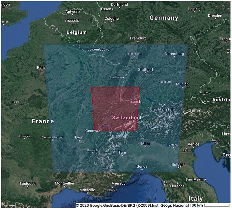
Figure 1. The analysis region over central Europe used in this study indicated with red box (temperature) and blue box (precipitation).

2.1.2. Observations

The observational data set used in this study is a gridded precipitation dataset for year 2004, covering the area of Switzerland. The horizontal grid spacing of the data is 1 km (Wüest et al., 2010) and it is available at hourly frequency. It is generated using a combination of station data with radar-based disaggregation. The data is often used for climate model evaluation (see e.g., Ban et al., 2014).

2.2. Supervised Machine Learning for Downscaling of Meteorological Data

Let X be a coarse patch with X × Y × T regular grid points, and let Y be the corresponding downscaled patch with $\overline{X}\times \overline{Y}\times \overline{T}$ grid points. Further, let f(Y) be a map that coarsens a high-resolution patch Y into its corresponding low-resolution patch X:

$\begin{array}{ll}{\displaystyle \underset{\text{coarsening}}{{\displaystyle \underbrace{\text{X}=f(\text{Y})}}}},{\displaystyle \underset{\text{downscaling}}{{\displaystyle \underbrace{\text{Y}=f^{-1}(\text{X})}}}}& (1)\end{array}$

The inverse problem f⁻¹, i.e., the downscaling problem, is usually ill-posed, since the map f is not bijective. While any high-resolution patch can be turned into a unique low-resolution patch via coarsening, the reverse will have multiple possible solutions, i.e., f is surjective, but not injective.

However, not every possible solution to Y = f⁻¹(X) is physically meaningful and realizable in real-world data. It therefore makes sense to construct the inverse map f⁻¹ in a data-driven manner from real-world data to only include mappings that have actually been seen during training, which is the key idea behind supervised machine learning. The inverse map is thereby parameterized by a concatenation of multiple weighted sums of inputs that each go through a non-linear mapping. The composition–a deep neural network–thereby becomes a differentiable, highly non-linear mapping between the input and output space, and can be iteratively trained via gradient descent.

The success of a deep neural network thereby hinges on three key criteria:

1. the architecture of the neural network combines low-frequent and high-frequent information, and the gradients dY/dX are well defined to facilitate the training process,

2. the training data is of high quality and expressive, i.e., we explore the space of possible mappings sufficiently and the mappings are sufficiently distinct.

3. the loss function expresses the desired goal well and the energy manifold is well-behaved to allow a stable (stochastic) gradient descent.

In the following subsections, we elaborate on the network architectures in section 2.2.1, the training data generation in section 2.2.2, and the training procedure and loss function in section 2.2.3.

2.2.1. Network Architecture

When observing meteorological variables, such as temperature and precipitation, we can see vast differences in their spatial and temporal variability. While temperature varies slowly in space and time, i.e., it is a comparatively low-frequent signal, precipitation is far more localized and varies faster, i.e., it is a high-frequent signal that is harder to predict with conventional downscaling techniques. To leverage the data characteristics, we design two separate convolutional neural networks to represent the inverse mapping f⁻¹.

2.2.1.1. Low-Frequent Data: Residual-Predicting Network (RPN)

In case, the data has low spatial and temporal variability, a conventional downscaling technique might already take us close to the desired solution. Rather than learning the entire downscaling process, it will then be an easier task to correct the conventional downscaling method, which is the core concept of residual learning (cf. Dong et al., 2015). Let ${\hat{f}}^{-1}$ be an existing downscaling technique, such as trilinear interpolation in space-time. Then, the inverse f⁻¹(X) can be formed by:

$\begin{array}{ll}{f}^{-1}(\text{X})={\displaystyle \underset{\text{trilinear downscaling}}{{\displaystyle \underbrace{{\hat{f}}^{-1}(\text{X})}}}}+{\displaystyle \underset{\text{residual}}{{\displaystyle \underbrace{r({\hat{f}}^{-1}(\text{X}))}}}}& (2)\end{array}$

where our neural network only learns to predict the residual $r({\hat{f}}^{-1}(\text{X}))$ of the trilinear downscaling method. For this, we follow the architecture of Mao et al. (2016), who applied an encoder-decoder architecture, which is detailed further below. The advantage of this approach is that it is comparatively easier to improve over the existing trilinear baseline method in contrast to learning a downscaling method from scratch. If ${\hat{f}}^{-1}(\text{X})$ performs poorly, for example since the scalar field exhibits too much temporal variability, then the next approach will perform better.

2.2.1.2. High-Frequent Data: Deconvolutional Network (DCN)

Consider a case in which too much motion occurred between time steps, e.g., a cloud got transported to a new location not overlapping with its previous location. Then, the trilinear downscaling method might interpolate two small clouds in the time step in-between at the original and the final location, rather than obtaining a single translating cloud in the middle. Other than before, the linear downscaling in time might not be close enough to benefit from residual prediction. In such cases where a a conventional temporal downscaling method is not helpful, we learn the partial mapping $p({\tilde{f}}^{-1}(\text{X}))$ from spatially-downscaled data to the high resolution:

$\begin{array}{ll}{f}^{-1}(\text{X})={\displaystyle \underset{\text{partial downscaling}}{{\displaystyle \underbrace{p({\tilde{f}}^{-1}(\text{X}))}}}}& (3)\end{array}$

where ${\tilde{f}}^{-1}(\text{X})$ performs only spatial downscaling using bilinear interpolation, but not temporal downscaling and where $p({\tilde{f}}^{-1}(\text{X}))$ performs both the temporal downscaling and improves over the result of ${\tilde{f}}^{-1}$. Since ${\tilde{f}}^{-1}(\text{X})$ does not interpolate information in time, a residual prediction is no longer applicable. Hence, the high-resolution data is predicted directly. For the network architecture, we follow a typical U-Net architecture (Ronneberger et al., 2015), which is a general design not limited to downscaling problems. In our downscaling setting, the input data is spatially downscaled with a bilinear baseline method, as was proposed by Lu and Chen (2019) for image super-resolution. In the following, we explain how the networks are structured and which modifications improved the performance for meteorological downscaling problems.

2.2.1.3. Layers and Skip Connections

The neural network architectures are illustrated in Figure 2. In both architectures, the network consists of convolutional layers only. Among the most recent convolutional neural network architectures, U-Nets by Ronneberger et al. (2015) are often the most promising approach. A U-Net extracts both low-frequency and high-frequency features from the data by repeatedly performing feature extraction and coarsening. In the so-called contraction phase, we apply successively two convolutional layers followed by a MaxPooling layer to extract features and then reduce the resolution. To handle convolutions on image boundaries, we use zero-padding and apply the convolutions with a stride of 1, i.e., every pixel of the input data will once be the center of a convolution kernel. We repeat this structure four times where the last time we omit the pooling layer. Within each layer, we extract a certain number of features. Starting with 64 features maps, we double the size until 512 feature maps are reached in the last layer. This is the amount of information available in the subsequent step: the synthesis of the output in the expansion phase. In the expansion phase, the goal is to reconstruct a high resolution image from all previously extracted features by iteratively increasing the number of grid points until the target resolution is reached. We do this by using so-called UpSampling layers, which repeat the values to a larger data block, followed by three convolutional layers. The key to success is to provide in each level of the U-Net the feature maps that have been extracted previously on the same resolution during contraction. This is achieved by skip connections from the contraction to the expansion phase. Adding the skip connections as in the U-Net by Ronneberger et al. (2015) has two positive effects. First, it was shown to smooth the loss landscape (c.f., Li et al., 2018), which makes it easier to perform gradient descent during training. Second, the skip connections give access to the high-frequency information of earlier layers, which greatly helps to construct high-frequent outputs.

FIGURE 2

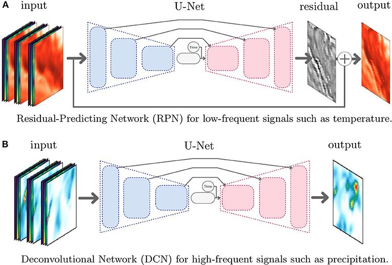
Figure 2. Illustrations of the convolutional neural network architectures for downscaling of low-frequent and high-frequent meteorological variables. Both architectures receive three time steps of the scalar field to predict (temperature or precipitation) and additional fields (longitude, latitude, surface height) as input. For RPN, the input data is downscaled conventionally in both space and time. For DCN, the input data is downscaled conventionally only in space. In both networks, the time variable is appended in the latent space and indicates at which relative time between the input frames the output should be downscaled at. (A) Residual-predicting network (RPN) for low-frequent signals, such as temperature. (B) Deconvolutional network (DCN) for high-frequent signals, such as precipitation.

2.2.1.4. Inputs and Outputs

Since we intend to downscale data both in space and time, we provide the network with both spatial and temporal information. Thus, the input to the model is a 4D data block, one dimension is used for the time steps, two for the spatial information, and the last one holds the so-called channels. A difference to the conventional U-Net is that we experimented with additional data channels that provide more information to resolve ambiguities in the inverse map f⁻¹. The effectiveness of additional data channels was already demonstrated by Vandal et al. (2017) and Höhlein et al. (2020) for downscaling. These additional channels include latitude and longitude such that the network can learn regional weather patterns, and altitude to include dependencies on the topography. For example, we observed that adding these additional fields improved the residual by 7.3%, for a precipitation downscaling with k_x = k_y = k_t = 4. In addition, we provide temporal information to the network, which allows us to give the model information about the relative time between the next known adjacent time steps. Since the time variable is a constant and not a spatially-varying map–unlike all other previously mentioned additional information, we append the time to the latent space, i.e., the feature map at the end of the feature extraction phase. Other options to include the time are imaginable. Including time as a constant separate slice in the input would increase the network size, which is why we opted for appending it to the latent space. Our data concentrated on a specific season. Including the day of the year as additional variable in order to learn seasonal effects would be straightforward to add.

The output of the network depends on the chosen architecture. As described above, we predict the error residual for the low-frequent data in the RPN, e.g., for the temperature field. In the case of high-frequent data, such as precipitation, we directly predict the high-resolution outputs in the DCN. In both cases, the networks are convolutional, thus the network can be applied at inference time to the full input domain at once.

2.2.2. Training Data Generation

Supervised machine learning requires groundtruth pairs of low-resolution and corresponding high-resolution patches. In the following, we describe how these groundtruth pairs are generated from the given high-resolution meteorological data. The coarsening operation depends on the units of the data. When the units remain the same (e.g., absolute temperature in K), then we use an average operation only. When the units change (e.g., total precipitation depends on the time step), then we apply averaging and convert the units afterwards. In case of precipitation, the coarsening in time is equal to an accumulation of the precipitation values. Generally, we recommend to use an averaging operation to do the coarsening, since a max operation or a simple subsampling would cause aliasing artifacts that would not be present if the data was simulated or measured on lower resolution. For the residual predicting network (RPN), we downscale the low-resolution data with a conventional trilinear interpolation method, and feed the downscaled data to the network in order to predict the residual (c.f., section Low-frequent data: residual-predicting network (RPN)). In this work, we applied linear interpolation to avoid extrapolation of minima and maxima. Any other existing downscaling method, such as cubic interpolation, would conceptually also be imaginable. For DCN, the network receives spatially-downscaled input, similar to RPN. In the temporal direction, we input the coarse resolution, since a linear interpolation would cause blending and ghosting artifacts that the network would have to learn to undo. During training, we randomly crop patches with a resolution of 32 × 32 from the high-resolution and (conventionally downscaled) low-resolution data. We thereby separate the time sequence into a training period and a testing period to assure that the training and testing sets are independent. For this, we used the last 10% of the time range for testing.

Since the input fields (temperature or precipitation, and longitude, latitude, and surface height) would have different value ranges, we normalize all fields globally across the entire data set to the unit interval [0, 1], which is a common preprocess with neural networks. The scaling factors are stored, such that the results of the network can be scaled back to the physical units later.

2.2.3. Training Procedure and Loss

As loss function, we measure the difference between the predicted result Y and the groundtruth $\overline{Y}$. Convolutional neural networks are known to oversmooth the output. Hence, we assess the difference with an L₁ norm that is combined with a gradient loss to not only penalize differences in the values but also in the derivatives, which aids in the reconstruction of higher-frequency details. We refer to Kim and Günther (2019) and Kim et al. (2019) for a discussion of the norms and weights of the gradient loss.

$\begin{array}{ll}{L}(\text{Y},\overline{\text{Y}})={\displaystyle \underset{\text{data loss}}{{\displaystyle \underbrace{|\text{Y}-\overline{\text{Y}}{|}_1}}}}+\lambda {\displaystyle \underset{\text{gradient loss}}{{\displaystyle \underbrace{|\nabla \text{Y}-\nabla \overline{\text{Y}}{|}_1}}}}& (4)\end{array}$

Here, λ is a weight indicating how much the focus should lie on the difference of gradients. We explored the residual for different choices of λ in a precipitation downscaling experiment with scaling factors 2 in temporal and spatial dimension. The baseline obtains a residual of 6.601 MSE [g/m²]. Setting λ = 0, i.e., not including the gradient loss term, gives the simple L1-norm, which obtains a residual of 8.181 MSE [g/m²], which is larger than the baseline. Thus, the gradient loss term is required such that the network is able to concentrate on high-frequent details. We empirically set λ = 1 in our experiments, which result in a residual of 3.882 MSE [g/m²]. Increasing λ further, e.g., to λ = 10, again increased the residual of the network to 5.846 MSE [g/m²].

As common with neural networks, we performed for both network architectures a hyperparameter optimization, i.e., we empirically adjusted each network parameter, such as the number of layers, the number of features, the batch size, and the activation functions to obtain the best neural network for each problem. Alternatively, automatic hyper-parameter optimization frameworks, such as Optuna are available (Akiba et al., 2019), which could be employed in the future. We choose Adam as optimizer with the default settings (learning rate 0.001) as proposed by Kingma and Ba (2014), and used a batch size of 8 to meet GPU memory constraints. Both networks were trained for 80 h on a single compute node (Intel Xeon CPU E5-2630, Nvidia GeForce 1080Ti). The training time is an important factor in the hyper-parameter optimization. Automatic frameworks, such as Optuna (Akiba et al., 2019), explore many different hyper-parameter combinations, each requiring a training run. For such an automatic hyper-parameter optimization, the total training time would scale linearly in the number of tested parameter configurations.

2.3. Analysis

To evaluate the neural networks, we performed a number of experiments, which are detailed in the following sections. To quantify the improvement over the trilinear downscaling in space-time, we calculate the mean squared error (MSE). Let i ∈ {1, …, n} be the index of the n grid points of a space-time patch, then MSE is defined as:

$\begin{array}{lll}MSE(\text{Y},\overline{\text{Y}})& =\frac{1}{n}{\displaystyle \sum _i^n}|{\text{Y}}_i-{\overline{\text{Y}}}_i{|}^2& (5)\end{array}$

where Y is the downscaled result and $\overline{\text{Y}}$ is the groundtruth. Along with the quantitative measures, we visualize the downscaled fields to show the amount of detail that is reconstructed visually.

To assess how well the network is able to downscale in space and in time, we vary the downscaling factors k_x, k_y, and k_t in an ablation study in sections 3.1.1 and 3.2.1, and train a network for each case separately. We can expect that small factors will perform better, since less information is missing. The networks were designed for low-frequent input data (RPN) and high-frequent input data (DCN). Therefore, we evaluate both networks on their respective data type, namely temperature fields for RPN, and the precipitation for DCN. To justify the need for DCN, we apply the RPN network to high-frequent precipitation data, as well. Likewise, we apply the DCN network to low-frequent temperature data.

Finally, we train neural networks for observational data in section 3.2.2. Compared to numerical data, observations exhibit very different data characteristics in terms of resolution, noise, and spatial and temporal variation.

3. Results

In this section, we report and discuss results of our experiments. We begin with experiments on low-frequent data (temperature), which is followed by reporting results for high-frequent data (precipitation). For all shown metrics, we compare with the high-resolution ground truth, which is equivalent to the result obtained by a full resimulation. A resimulation is prohibitively expensive, taking a full day on Piz-Daint (supercomputer at the Swiss National Supercomputing Center (CSCS) in Switzerland) utilizing 100 GPU nodes (Nvidia Tesla K20X).

3.1. Temperature

First, we investigate the downscaling capabilities for both network architectures by reporting the residual errors for different downscaling factors.

3.1.1. Network Comparison

We reduced the number of spatial grid points by a factor of 2 and 4, and the time steps by a factor of 2, 4, and 12. For all scaling factors, we perform downscaling with the baseline method and our two network architectures, and report the MSE (in °C) in Table 1. With only temporal downscaling (k_x = k_y = 1), RPN and the baseline give similar results, while DCN is about 80% worse. Across all spatial downscaling factors, varying the temporal downscaling does not significantly change the result, since the temporal variation of temperature was low. Compared to the baseline, RPN is able to reduce the error for k_x = k_y = 2 by about 58%, while DCN achieves 53%. A more significant difference occurs for spatial downscaling with k_x = k_y = 4, for which RPN achieves 64% and DCN only 41% reduction compared to the baseline (cf. Table 1). In Figure 3A, we see at the example of k_x = k_y = 2, k_t = 4 that both networks achieve a reasonable reduction of the loss. RPN improves over the DCN architecture in both the convergence rate and the obtained residual. We can observe that for a low-frequent signal, such as temperature, the residual predicting network (RPN) consistently outperforms the baseline and the deconvolutional approach (DCN). The only exception occurred for k_x = k_y = 1 (no spatial down-scaling) and k_t = 2 (temporal down-scaling by factor 2). Since temperature varies very slowly in time, the baseline already obtains a very small error. In that case, RPN is on average 0.001°C worse than the baseline (only yellow square for RPN in Table 1), which is a negligible difference. We can also see that a reconstruction from a high temporal coarsening (k_t = 12, k_x = k_y = 2) is better than the reconstruction from larger spatial coarsening (k_t = 1, k_x = k_y = 4), which would both reconstruct from the same number of low-resolution grid points. This is because temperature changes slower over time, therefore downscaling in this dimension is easier for the neural network to learn.

TABLE 1

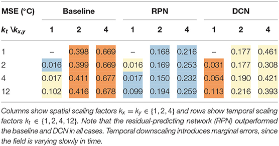
Table 1. Temperature (°C) downscaling mean-squared errors (MSE), coloring the best ($•$), intermediate ($•$) and worst ($•$) result.

FIGURE 3

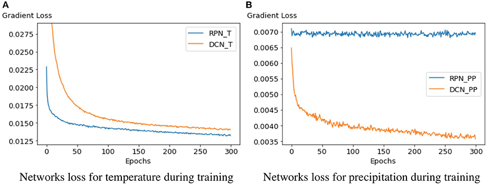
Figure 3. Validation loss plots of both architectures on temperature and precipitation. The left plot shows that RPN converges faster and achieves a lower loss during training for the temperature field than DCN. On the other hand, we see that the same RPN architecture is unable to learn when applied on precipitation data. (A) Network loss for temperature during training. (B) Network loss for precipitation during training.

In addition to the quantitative measures, we provide a qualitative view onto the reconstructed temperature field. Figure 4 shows a sample of the testing set with a spatial and temporal downscaling factor of k_x = k_y = k_t = 4. The RPN model is able to recover detailed structures, increasing the quality not only quantitatively but also visually. The corresponding error map in Figure 5 shows that the remaining errors remain highest in regions with complex topography due the high spatial variability. The MSE reduced by a factor of 10.

FIGURE 4

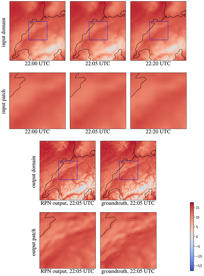
Figure 4. Downscaling results for temperature (in °C) by a factor of k_x = k_y = k_t = 4 in both the temporal and spatial dimension. The first row shows time steps of the trivially downscaled domain. The second row shows a patch as it is sent into the network. The third row compares the result of the network to the groundtruth on the full domain. The last row shows the groundtruth comparison for the patch that was predicted.

FIGURE 5

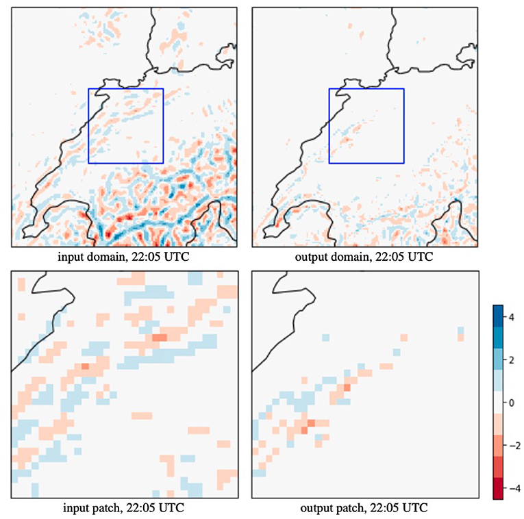
Figure 5. The error map of Figure 4 in MSE (°C) shows a comparison between the trilinear interpolated input and our predicted output relative to the groundtruth. On the full domain, RPN reduces the MSE from 1.438 to 0.143°C which is a 10× improvement, and on the zoom-in (blue box), the MSE reduced from 0.533 to 0.077°C.

The reconstruction of temperature data can be done in parallel and takes 1 min on a single Intel i7 4770 HQ (2.2 GHz) per timestep, while the network requires about 125 MB of storage.

3.2. Precipitation

In this section, we study a more challenging task: the downscaling of high-frequent precipitation fields.

3.2.1. Network Comparison

The numerical precipitation data was given at 5 min intervals. For temporal downscaling, we test the reconstruction from 10, 20 min, and hourly data. In Table 2, we report the MSE for the baseline, RPN and DCN for multiple combinations of downscaling factors. While the low-frequent temperature field was best reconstructed by residual learning using RPN, the technique fails on the high-frequent precipitation field, increasing the error on average by a factor of two. Using the DCN architecture instead, consistently leads to better results. For k_x = k_y = 1, the DCN improved over the baseline on average by about 43%, for k_x = k_y = 2 by about 54%, and for k_x = k_y = 4 by about 47%. The less the spatial dimension was downscaled, the higher the improvement when increasing the temporal downscaling. Thus, other than for RPN and low-frequent fields, here, the temporal factor is more important. For example with DCN, we induce more error when reconstructing from a coarsening with a temporal factor to 12 (k_t = 12, k_x = k_y = 2) than when reconstructing from a coarsening with a spatial factor of four (k_t = 4, k_x = k_y = 4), although the total number of grid points to start from was larger for k_t = 12, k_x = k_y = 2. In Figure 3B, we see at the example of k_x = k_y = 2, k_t = 4 that only the DCN network was able to learn for precipitation fields, and that the same RPN architecture that was used before on temperature was not able to reduce the loss, which explains the higher errors of RPN compared to the baseline.

TABLE 2

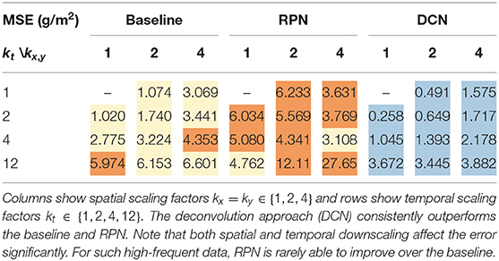
Table 2. Precipitation (g/m²) downscaling mean-squared errors (MSE), coloring the best ($•$), intermediate ($•$) and worst ($•$) result.

Figure 6 shows an example of downscaling from 20 to 5 min. The time steps that are sent into the network shown, in which a cloud movement from the top left to the bottom right is apparent, as well as how precipitation decreases over time. Using this information, the DCN network is able to estimate the position and the amount of precipitation at a specific intermediate time. Figure 7 shows the error map of a conventional linear downscaling and our neural network prediction, where we can see that the DCN output is closer to the ground truth.

FIGURE 6

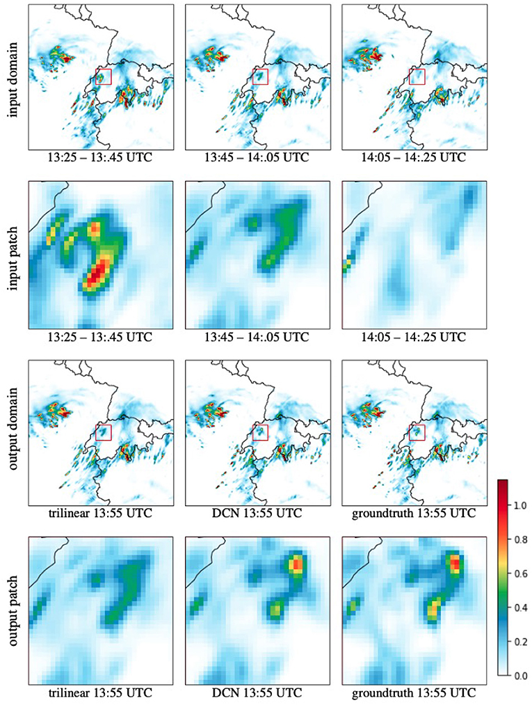
Figure 6. Downscaling results for precipitation (g/m²) by a factor of k_t = 4 from 20 to 5 min resolution. The first row shows time steps of the trivially downscaled domain (spatially). The second row shows a patch as it is sent into the network. The third row compares the result of the network to the groundtruth on the full domain. The last row shows the groundtruth comparison for the patch that was predicted.

FIGURE 7

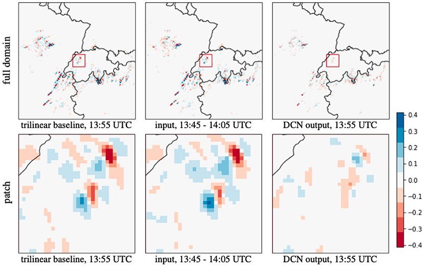
Figure 7. The error map of Figure 6 compares the trilinear interpolated baseline, the time-integrated network input covering the time to predict, and our predicted output. DCN reduces the MSE from 2.269 to 0.745 g/m² on the full domain, and from 4.531 to 0.910 g/m² in the shown patch.

3.2.2. Application of Deep Learning to Observational Data

Given the experiments on simulated data, another interesting question is to see if the model is able to learn how to downscale observational data. For this, we run eight instances of our model training on the observational data and performed downscaling between different pairs of resolutions. We checked how the model can downscale from 2, 4, 6, 12, and 24 hourly data to 1 h intervals. Additionally, we evaluated the downscaling from 12 and 24 h data to 6 h data, and from 24 h data to 12 h. The results are summarized in Table 3. We observe that for small downscaling factors like from 2 to 1 h data, our model is able to reduce the error compared to the baseline by 24.65%. Increasing the downscaling factor decreases the performance and gets worse for high factors like 12 or 24–1 h data. For such extreme downscaling, not enough information is present to disambiguate the correct hourly information. When downscaling smaller factors but on coarser resolution, i.e., with a downscaling factor of 2 but from 12 to 6 h data, the model is able to improve significantly over the baseline and for the extreme case of downscaling from daily data to 12 h data it achieved an error reduction of up to 70%. Figure 8 shows an example of this downscaling scenario.

TABLE 3

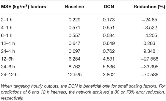
Table 3. Observation downscaling results in temporal dimension, using the baseline and our DCN.

FIGURE 8

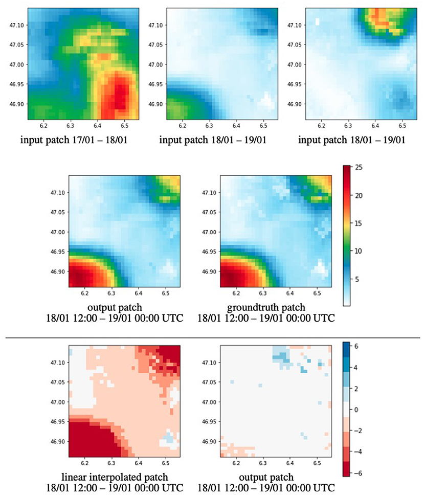
Figure 8. Downscaling results of observational precipitation from 24 h resolution to 12 h. Top row shows input patches ranging from 1 day 12:00 UTC to the other 12:00 UTC. Middle row shows the predicted output patch and the groundtruth. Last row compares the baseline and predicted error maps relative to the groundtruth (MSE kg/m²). Our method learns to scale the amount of precipitation dependent on the time we estimate. Our method can reduce the MSE from 14.251 to 0.252.

4. Conclusions

In this paper, we investigated the suitability of deep learning for the reconstruction of numerically-simulated and observed low-resolution data in both space and time. We thereby concentrated on two meteorological variables—temperature and precipitation—for which we develop suitable network architectures that utilize additional time-invariant information, such as the topography. We decided on temperature and precipitation to assess the performance of a neural network on both low-frequent and very high-frequent fields in order to test the limits of the architectures. While we observed that slowly-changing information, such as temperature can be adequately predicted through an error-predicting network, we found that fields with larger variations in both space and time, such as precipitation, require a different approach and cannot profit from residual learning, as there is no straight-forward downscaling method to leverage which achieves close enough baselines. Learning to suppress unnecessary or wrong structures is more difficult, then letting the network directly predict the high-resolution output by itself from the extracted features. For both cases, we developed a convolutional architecture with residual skip connections in order to extract features at different scales and to combine them in the subsequent deconvolution, leading us to a high-resolution prediction.

One possible reason why data is available at lower resolution only is that it has been coarsened for storage. If storage alone was the concern, it would be more effective to apply lossy compression approaches directly to the high-resolution data, especially if the data has low-frequent regions that could be sampled more sparsely than the uniformly chosen coarse resolution used throughout this manuscript for coarsening. That said, a limitation of the presented downscaling approach is that it is not able to compete with lossy compressions that were able to work from the high-resolution data. Instead, we focused on what can be recovered once the damage is done, i.e., once the data has been coarsened. Future work could follow up on the compression, for which an information theoretic approach would be instructive (MacKay, 2003; Yeung, 2010). In the future, it would be interesting to study if there are ways to predict the optimal downscaling parameters. This will be quite challenging, since the best network and the best parameter choice is strongly dependent on the data characteristics, which vary not only spatially but also temporally.

At present, we assumed that the meteorological data is available on regular grids. In such a case, convolutional layers proved useful for feature map extraction in the hidden layers. In the future, it would be interesting to study convolutional approaches for unstructured or irregularly structured data. Possible approaches would include PointNet-like convolutions (Qi et al., 2017) that waive connectivity information by introducing order-independent aggregations, or graph convolutional networks (Kipf and Welling, 2016) that operate on arbitrary grid topologies.

CNNs and GANs similarly share the problem that their interpretation is difficult, since both involve nonlinear mappings. For example, both of our CNN approaches RPN and DCN obtain an error that is theoretically unbounded. It would be imaginable to bound the reconstruction heuristically using the coarse input data, for example by only allowing a certain deviation away from the input signal, but this would of course be rather heuristic. Extreme weather events could be smoothed out since the frequency of their occurrence was not accounted for in the training data. Weighting individual training samples is an interesting direction for future work, which would require more data and an identification of the extreme events.

Neural networks can learn to disambiguate the reconstruction from low-resolution to high-resolution data in a data-driven way. In the future, it would be interesting to include additional regularizers into the loss function to utilize physical conservation laws that needed to hold during simulation. Further, it would be interesting to apply residual predictions to dynamical downscaling models, as this would build up on the meteorological knowledge that went into the design of dynamical models. While running the dynamical models also imposes a computational cost, there is great potential in including more physics into the learning process.

The work presented here shows a proof of concept how neural networks can be used to reconstruct data that has been coarsened, and how this could serve for development/reconstruction of high-resolution model data and observations. For example, trained networks can be used for disaggregation of daily observational values into subdaily instead of using functions that can introduce statistical artifacts. It still remains to expand the current study to different domains and to longer time periods and it still remains an open problem to investigate if and how the hallucinations of generative neural networks (Singh et al., 2019; Han and Wang, 2020; Stengel et al., 2020) might impede the data analysis.

Data Availability Statement

The data analyzed in this study is subject to the following licenses/restrictions: gridded precipitation observations are obtained through MeteoSwiss data service. The data is available for research upon signing a license agreement. Due to the high data volume, the COSMO model data is available on request from the authors. The source code for the construction of the DCN and RPN, as well as the gradient loss calculation are available on GitHub at http://github.com/aserifi/convolutional-downscaling. Requests to access these datasets should be directed to the authors.

Author Contributions

AS conducted the analysis and wrote the manuscript. TG conceived the idea and NB provided the data. TG and NB have supervised the work with regular inputs and have contributed to the writing of the manuscript. All authors contributed to the article and approved the submitted version.

Funding

This work was supported by the Swiss National Science Foundation (SNSF) Ambizione grant no. PZ00P2_180114.

Conflict of Interest

The authors declare that the research was conducted in the absence of any commercial or financial relationships that could be construed as a potential conflict of interest.

Acknowledgments

We acknowledge PRACE for awarding us access to Piz Daint at Swiss National Supercomputing Center (CSCS, Switzerland). We also acknowledge the Federal Office for Meteorology and Climatology MeteoSwiss, the Swiss National Supercomputing Centre (CSCS), and ETH Zürich for their contributions to the development of the GPU-accelerated version of COSMO.

References

Akiba, T., Sano, S., Yanase, T., Ohta, T., and Koyama, M. (2019). “Optuna: a next-generation hyperparameter optimization framework,” in Proceedings of the 25th ACM SIGKDD International Conference on Knowledge Discovery & Data Mining (Anchorage, AK), 2623–2631. doi: 10.1145/3292500.3330701

CrossRef Full Text | Google Scholar

Ban, N., Schmidli, J., and Schär, C. (2014). Evaluation of the convection-resolving regional climate modeling approach in decade-long simulations. J. Geophys. Res. Atmos. 119, 7889–7907. doi: 10.1002/2014JD021478

CrossRef Full Text | Google Scholar

Baño-Medina, J. L., García Manzanas, R., and Gutiérrez Llorente, J. M. (2020). Configuration and intercomparison of deep learning neural models for statistical downscaling. Geosci. Model Dev. 13, 2109–2124. doi: 10.5194/gmd-2019-278

CrossRef Full Text | Google Scholar

Cheng, J., Kuang, Q., Shen, C., Liu, J., Tan, X., and Liu, W. (2020). Reslap: generating high-resolution climate prediction through image super-resolution. IEEE Access 8, 39623–39634. doi: 10.1109/ACCESS.2020.2974785

CrossRef Full Text | Google Scholar

Dong, C., Loy, C. C., He, K., and Tang, X. (2015). Image super-resolution using deep convolutional networks. IEEE Trans. Pattern Anal. Mach. Intell. 38, 295–307. doi: 10.1109/TPAMI.2015.2439281

PubMed Abstract | CrossRef Full Text | Google Scholar

Fuhrer, O., Osuna, C., Lapillonne, X., Gysi, T., Cumming, B., Bianco, M., et al. (2014). Towards a performance portable, architecture agnostic implementation strategy for weather and climate models. Supercomput. Front. Innov. 1, 45–62. doi: 10.14529/jsfi140103

CrossRef Full Text | Google Scholar

Han, J., and Wang, C. (2020). SSR-TVD: spatial super-resolution for time-varying data analysis and visualization. IEEE Trans. Vis. Comput. Graph. doi: 10.1109/TVCG.2020.3032123. [Epub ahead of print].

PubMed Abstract | CrossRef Full Text | Google Scholar

Hentgen, L., Ban, N., and Schär, C. (2019). Clouds in convection resolving climate simulations over Europe. J. Geophys. Res. Atmos. 124, 3849–3870. doi: 10.1029/2018JD030150

CrossRef Full Text | Google Scholar

Höhlein, K., Kern, M., Hewson, T., and Westermann, R. (2020). A comparative study of convolutional neural network models for wind field downscaling. Meteorol. Appl. 27:e1961. doi: 10.1002/met.1961

CrossRef Full Text | Google Scholar

Kim, B., Azevedo, V. C., Thuerey, N., Kim, T., Gross, M., and Solenthaler, B. (2019). Deep fluids: a generative network for parameterized fluid simulations. Comput. Graph. Forum 38, 59–70. doi: 10.1111/cgf.13619

CrossRef Full Text | Google Scholar

Kim, B., and Günther, T. (2019). Robust reference frame extraction from unsteady 2D vector fields with convolutional neural networks. Comput. Graph. Forum 38, 285–295. doi: 10.1111/cgf.13689

CrossRef Full Text | Google Scholar

Kingma, D. P., and Ba, J. (2014). Adam: a method for stochastic optimization. arXiv 1412.6980.

Google Scholar

Kipf, T. N., and Welling, M. (2016). Semi-supervised classification with graph convolutional networks. arXiv 1609.02907.

PubMed Abstract | Google Scholar

Leutwyler, D., Lüthi, D., Ban, N., Fuhrer, O., and Schär, C. (2017). Evaluation of the convection-resolving climate modeling approach on continental scales. J. Geophys. Res. Atmos. 122, 5237–5258. doi: 10.1002/2016JD026013

CrossRef Full Text | Google Scholar

Li, H., Xu, Z., Taylor, G., Studer, C., and Goldstein, T. (2018). “Visualizing the loss landscape of neural nets,” in Proceedings of the 32nd International Conference on Neural Information Processing Systems (Red Hook, NY: Curran Associates Inc.), 6391–6401. doi: 10.5555/3327345.3327535

CrossRef Full Text | Google Scholar

Lu, Z., and Chen, Y. (2019). Single image super resolution based on a modified U-net with mixed gradient loss. arXiv 1911.09428.

Google Scholar

Ma, K. (2009). In situ visualization at extreme scale: challenges and opportunities. IEEE Comput. Graph. Appl. 29, 14–19. doi: 10.1109/MCG.2009.120

PubMed Abstract | CrossRef Full Text | Google Scholar

MacKay, D. J. (2003). Information Theory, Inference and Learning Algorithms. Cambridge: Cambridge University Press.

Google Scholar

Mailhot, A., and Duchesne, S. (2010). Design criteria of urban drainage infrastructures under climate change. J. Water Resour. Plan. Manage. 136, 201–208. doi: 10.1061/(ASCE)WR.1943-5452.0000023

CrossRef Full Text | Google Scholar

Mao, X. J., Shen, C., and Yang, Y. B. (2016). Image restoration using very deep convolutional encoder-decoder networks with symmetric skip connections. arXiv 1603.09056.

Google Scholar

Min, M., Li, J., Wang, F., Liu, Z., and Menzel, W. P. (2020). Retrieval of cloud top properties from advanced geostationary satellite imager measurements based on machine learning algorithms. Rem. Sens. Environ. 239:111616. doi: 10.1016/j.rse.2019.111616

CrossRef Full Text | Google Scholar

O'Gorman, P. A., and Dwyer, J. G. (2018). Using machine learning to parameterize moist convection: potential for modeling of climate, climate change, and extreme events. J. Adv. Model. Earth Syst. 10, 2548–2563. doi: 10.1029/2018MS001351

CrossRef Full Text | Google Scholar

Pouliot, D., Latifovic, R., Pasher, J., and Duffe, J. (2018). Landsat super-resolution enhancement using convolution neural networks and sentinel-2 for training. Rem. Sens. 10:394. doi: 10.3390/rs10030394

CrossRef Full Text | Google Scholar

Prein, A. F., Langhans, W., Fosser, G., Ferrone, A., Ban, N., Goergen, K., et al. (2015). A review on regional convection-permitting climate modeling: demonstrations, prospects, and challenges. Rev. Geophys. 53, 323–361. doi: 10.1002/2014RG000475

PubMed Abstract | CrossRef Full Text | Google Scholar

Qi, C. R., Yi, L., Su, H., and Guibas, L. J. (2017). Pointnet++: deep hierarchical feature learning on point sets in a metric space. arXiv 1706.02413.

Google Scholar

Rodrigues, E. R., Oliveira, I., Cunha, R., and Netto, M. (2018). “Deepdownscale: a deep learning strategy for high-resolution weather forecast,” in 2018 IEEE 14th International Conference on e-Science (e-Science) (Amsterdam: IEEE), 415–422. doi: 10.1109/eScience.2018.00130

CrossRef Full Text | Google Scholar

Roesch, I., and Günther, T. (2019). Visualization of neural network predictions for weather forecasting. Comput. Graph. Forum 38, 209–220. doi: 10.1111/cgf.13453

CrossRef Full Text | Google Scholar

Ronneberger, O., Fischer, P., and Brox, T. (2015). “U-Net: Convolutional networks for biomedical image segmentation,” in International Conference on Medical Image Computing and Computer-Assisted Intervention (Munich: Springer), 234–241. doi: 10.1007/978-3-319-24574-4_28

CrossRef Full Text | Google Scholar

Sachindra, D., Ahmed, K., Rashid, M. M., Shahid, S., and Perera, B. (2018). Statistical downscaling of precipitation using machine learning techniques. Atmos. Res. 212, 240–258. doi: 10.1016/j.atmosres.2018.05.022

CrossRef Full Text | Google Scholar

Schär, C., Fuhrer, O., Arteaga, A., Ban, N., Charpilloz, C., Di Girolamo, S., et al. (2020). Kilometer-scale climate models: prospects and challenges. Bull. Am. Meteorol. Soc. 101, E567–E587. doi: 10.1175/BAMS-D-18-0167.2

CrossRef Full Text | Google Scholar

Seifert, A., and Rasp, S. (2020). Potential and limitations of machine learning for modeling warm-rain cloud microphysical processes. J. Adv. Model. Earth Syst. 12:e2020MS002301. doi: 10.1029/2020MS002301

CrossRef Full Text | Google Scholar

Selbesoglu, M. O. (2019). Prediction of tropospheric wet delay by an artificial neural network model based on meteorological and gnss data. Eng. Sci. Technol. 23, 967–972. doi: 10.1016/j.jestch.2019.11.006

CrossRef Full Text | Google Scholar

Shi, W., Caballero, J., Theis, L., Huszar, F., Aitken, A., Ledig, C., et al. (2016). Is the deconvolution layer the same as a convolutional layer? arXiv 1609.07009.

Google Scholar

Singh, A., White, B. L., and Albert, A. (2019). “Downscaling numerical weather models with GANs,” in AGU Fall Meeting 2019 (San Francisco, CA: AGU).

Google Scholar

Stengel, K., Glaws, A., Hettinger, D., and King, R. N. (2020). Adversarial super-resolution of climatological wind and solar data. Proc. Natl. Acad. Sci. U.S.A. 117, 16805–16815. doi: 10.1073/pnas.1918964117

PubMed Abstract | CrossRef Full Text | Google Scholar

Steppeler, J., Doms, G., Schattler, U., Bitzer, H., Gassmann, A., Damrath, U., et al. (2003). Meso-gamma scale forecasts using the nonhydrostatic model LM. Meteor. Atmos. Phys. 82, 75–96. doi: 10.1007/s00703-001-0592-9

CrossRef Full Text | Google Scholar

Toderici, G., Vincent, D., Johnston, N., Jin Hwang, S., Minnen, D., Shor, J., et al. (2017). “Full resolution image compression with recurrent neural networks,” in Proceedings of the IEEE Conference on Computer Vision and Pattern Recognition (Honolulu, HI), 5306–5314. doi: 10.1109/CVPR.2017.577

CrossRef Full Text | Google Scholar

Vandal, T., Kodra, E., and Ganguly, A. R. (2019). Intercomparison of machine learning methods for statistical downscaling: the case of daily and extreme precipitation. Theor. Appl. Climatol. (Halifax, NS) 137, 557–570. doi: 10.1007/s00704-018-2613-3

CrossRef Full Text | Google Scholar

Vandal, T., Kodra, E., Ganguly, S., Michaelis, A., Nemani, R., and Ganguly, A. R. (2017). “DeepSD: generating high resolution climate change projections through single image super-resolution: an abridged version,” in International Joint Conferences on Artificial Intelligence Organization. doi: 10.1145/3097983.3098004

CrossRef Full Text | Google Scholar

Wang, Y., Perazzi, F., McWilliams, B., Sorkine-Hornung, A., Sorkine-Hornung, O., and Schroers, C. (2018). “A fully progressive approach to single-image super-resolution,” in Proceedings of the IEEE Conference on Computer Vision and Pattern Recognition Workshops (Salt Lake City, UT), 864–873. doi: 10.1109/CVPRW.2018.00131

CrossRef Full Text | Google Scholar

Wang, Y., Wang, L., Wang, H., and Li, P. (2019). End-to-end image super-resolution via deep and shallow convolutional networks. IEEE Access 7, 31959–31970. doi: 10.1109/ACCESS.2019.2903582

CrossRef Full Text | Google Scholar

Weyn, J. A., Durran, D. R., and Caruana, R. (2019). Can machines learn to predict weather? Using deep learning to predict gridded 500-HPA geopotential height from historical weather data. J. Adv. Model. Earth Syst. 11, 2680–2693. doi: 10.1029/2019MS001705

CrossRef Full Text | Google Scholar

Wüest, M., Frei, C., Altenhoff, A., M.Hagen, Litschi, M., and Schär, C. (2010). A gridded hourly precipitation dataset for Switzerland using rain-gauge analysis and radar-based disaggregation. Int. J. Climatol. 30, 1764–1775. doi: 10.1002/joc.2025

CrossRef Full Text | Google Scholar

Yang, C. Y., Ma, C., and Yang, M. H. (2014). “Single-image super-resolution: a benchmark,” in European Conference on Computer Vision (Springer), 372–386. doi: 10.1007/978-3-319-10593-2_25

CrossRef Full Text | Google Scholar

Yang, W., Zhang, X., Tian, Y., Wang, W., Xue, J.-H., and Liao, Q. (2019). Deep learning for single image super-resolution: a brief review. IEEE Trans. Multimed. 21, 3106–3121. doi: 10.1109/TMM.2019.2919431

CrossRef Full Text | Google Scholar

Yeung, R. W. (2010). Information Theory and Network Coding, 1st Edn. Springer Publishing Company, Incorporated.

Google Scholar

Yuval, J., O'Gorman, P. A., and Hill, C. N. (2021). Use of neural networks for stable, accurate and physically consistent parameterization of subgrid atmospheric processes with good performance at reduced precision. Geophys. Res. Lett. 48:e2020GL091363. doi: 10.1029/2020GL091363

CrossRef Full Text | Google Scholar