Relevance-Based Data Masking: A Model-Agnostic Transfer Learning Approach for Facial Expression Recognition

1. Introduction

In recent years deep learning approaches, have become a popular choice in the field of automatic emotion recognition. Among other things, Convolutional Neural Network (CNN) architectures are promising to overcome the limitations of handcrafted features by directly learning suitable representations from raw data. However, to train a CNN that handles such raw data input with high accuracy from scratch, vast amounts of annotated data are necessary as the absence of handcrafted features requires additional abstraction layers to be automatically learned by the network. In practice however it is relatively rare to have a dataset of sufficient size available for the specific task a network should be trained for. A common solution to this problem comes in the form of transfer learning where the previously gained knowledge of a model about related tasks is used to facilitate the learning process.

Specifically there are three potential benefits that can be gained from transfer learning (Torrey and Shavlik, 2010): Increased initial performance of the new model, a steeper learning slope that leads to faster learning and an increase in the final performance level that the model can achieve. For CNNs there are two major transfer learning strategies to be considered: The first one is to use a pretrained network as a feature extractor by only replacing the last fully-connected layers of the network. The second strategy is called fine tuning. Here, the Network is first trained on the related task and then fine-tuned to the target task by training on the target data. While either of those methods has been successfully applied to improve the state-of-the-art for a variety of recognition tasks, there are some limitations that need to be considered. When using a pretrained network for transfer learning the constrictions of the specific architecture are also inherited by the final model. Since the pretrained model is at least partially included in the structure of the final model, a change of architecture later on will therefore always require a complete retraining of the initial model. Modern CNN-Architectures can easily take up to multiple weeks to fully train, which makes such a complete retraining process rather time consuming or even unfeasible without the respective hardware equipment available. The second limitation is, that the learned knowledge can only be shared amongst neural networks—at least when applying finetuning. It is therefore not possible to transfer knowledge from other sources like different machine learning models or even humans directly into the process.

Such human knowledge could for example come in the form of visual attention. Eye movement studies have shown that humans fixate particular regions of the face in order to detect emotions (Green and Phillips, 2004). Drawing on knowledge about human attention, a neural network should be more sensitive to the relevant parts of a face and less sensitive to others. In fact, previous studies have shown that deep learning architectures with an attention mechanism can lead to significant improvements in performance over previous deep learning models (Minaee and Abdolrashidi, 2019). However, this attention is usually learned during the training process and can not be easily transferred from one model to the other to improve performance.

In this work we are presenting a model-agnostic, generalizable methodology to transfer learned knowledge of important regions from one model to another. Overall, our paper consists of three contributions:

1. We present a novel method to inject knowledge about the salience of facial regions that are relevant for emotion recognition from an arbitrary source into the training of a new model. This way we are able to accelerate the training process by forcing the neural network to focus on the relevant parts of the input.

2. We conducted a preliminary eye tracking study to obtain information on the human attentional process. Based on the results of this study we are presenting a method to automatically identify regions within the face that were relevant for a human annotator.

3. To avoid costly labeling we developed an approach to combine this information with saliency mapping techniques from the research field of Explainable Artificial Intelligence to assess the regions of the input that are most relevant for the decision of a pretrained neural network. This way we are able to simulate the attentional processes of humans when transferring knowledge from one model to another.

2. Related Work

Classical transfer learning approaches have been successfully applied for the task of automatically recognizing emotions for quite some time.

For instance, Ng et al. (2015) pretrained a deep Convolutional Neural Network on the generic ImageNet dataset. By successively first finetuning the network on an emotion recognition related auxiliary dataset and then on the final target dataset, they were able to achieve significant improvements over the proposed baseline.

Another approach was proposed by Xu et al. (2015), who trained deep CNNs to identify different faces in images and then transferred the high level features to recognize facial expressions. For training a facial expression detection system, they then used those networks as feature extractors to feed a support vector machine. In a study performed on a self recorded corpus they found, that their model not only performed significantly better than traditional approaches but was also more robust against occlusions that covered part of the face.

However, those methods have the common shortcoming that the architecture of the pretrained model is inherited by the final model and can therefore not be adapted easily. Another method of transferring knowledge between models, that is closely related to our approach and overcomes those limitations is Teacher-Student learning, also sometimes called Knowledge Distillation. Here a student-model is trained on the predictions of a teacher model instead of an annotated gold standard to transfer knowledge between models. While originally developed for model-compression (Buciluǎ et al., 2006) this approach has also been shown to achieve similar benefits as traditional transfer learning.

Li et al. (2017) employed a Teacher-Student model to adapt a speech recognition model to a new domain. In their experiments they evaluated the proposed approach in two scenarios. Firstly they adapted a clean acoustic model to noisy speech. In the second scenario they used adult's speech to adapt to children's speech. As a result of their experiments they observed a significant improvement in accuracy.

Meng Z. et al. (2019) used a “smart” Teacher-Student model for domain adaption and speaker adaption in automatic speech recognition. Their model selectively chooses to learn from either the teacher model or the gold standard labels conditioned on whether the teacher can correctly predict the gold standard. That way they achieved significant improvements for the respective tasks.

Similar to the adaption of noisy domains, Ge et al. (2018) used a selective-knowledge distillation model to recognize low-resolution faces. For that, they trained a teacher model on high resolution images and distilled the most relevant features into a student model for the recognition of specific faces in resolution-degraded images.

Albanie et al. (2018) exploited the idea that the emotional content of speech correlates with the facial expression of the speaker to develop a cross-modal Teacher-Student model for automatic emotion recognition. By using a trained model for automatic facial expression recognition as a Teacher, they created labels for the visual domain of video data to train the Student on the corresponding audio data. Their completely unsupervised approach achieved reasonable results on various standard benchmarks.

While these Teacher-Student approaches can be very effectively employed to compress knowledge that has been learned by large and complex models into smaller and more efficient ones, the transfer itself is performed indirectly via labels. In contrast to traditional fine tuning approaches, this does not necessarily reduce the time that is needed to train a model till convergence.

Besides transferring learned knowledge between models, attention mechanisms have been a popular approach recently to achieve similar benefits. Attention mechanisms are a component of a network's architecture that is responsible for guiding the networks attention to specific regions of interest in the input. For computer vision tasks attention can be loosely compared to the human visual attention mechanism that is capable of quickly parsing the field of view, discarding irrelevant information, and then focusing on a specific target region of interest to process (Itti and Koch, 2001).

Such a focus system for automatic facial expression recognition has been proposed by Minaee and Abdolrashidi (2019). By implementing an attention mechanism into a convolutional neural network they guided their network to pay more attention to task-relevant regions of the face, which resulted in significant improvements in classification performance over previous models on multiple datasets (FER, CKPlus, FERG, and JAFFE).

Meng D. et al. (2019) recently conducted a study on the effectiveness of attention for facial expression recognition in video sequences of variable length. Their Frame Attention Network used a self-attention and a relation-attention mechanism to identify the most relevant regions within a frame as well as the relevance of certain features within a global representation for the given video. Their tests on the CKPlus dataset showed that the addition of the self-attention module increased the classification performance significantly. Also adding the relation-attention module additionally increased performance beyond the state-of-the-art for this dataset.

Li et al. (2018) developed multiple approaches that dynamically redirect the attention of a CNN to clearly visible facial regions, to enhance facial expression recognition in case that the face in the input image might be obstructed. To evaluate their models they conducted experiments on multiple corpora, including the CKPlus and AffectNet dataset. The results of those experiments showed all their attention-based systems effectively outperforming other state-of-the-art methods. A visualization of the learned attention maps further more revealed that their models indeed learned to shift their focus onto the unobstructed part of an image in case the face was not clearly visible.

Fernandez et al. (2019) used the learned attention of a network to remove irrelevant parts of the input data before the final classification step. During their experiments on the CKPlus corpus they found that the attention module improved the overall system classification performance and noise-robustness of the model.

3. Overview of our Approach

In this section we present a generic method to assess the relevance of specific areas in the input and integrate this knowledge into a new model during training. Based on previous work from Schiller et al. (2019) our approach utilizes saliency maps generated by XAI algorithms like deep Taylor decomposition. These maps aim to identify the parts of the input that were relevant for a specific decision of a neural network. Inspired by findings that the human learning process can be accelerated by providing visual cues (Mac Aodha et al., 2018) we aim to use those saliency maps to guide the attention of a Trainee network, which we want to focus on areas that were relevant for another model that has been pretrained on a similar task.

The overall architecture for our method is illustrated in Figure 1. In the first step we are using the model, from which we want to extract the knowledge, to classify a given input sample. We refer to this model as the Trainer. Based on the prediction of our Trainer, we then create a saliency map that assigns a relevance value to each pixel of the input image, with respect to how relevant this pixel was for the specific decision of the model. For our experiments, we did this by performing a deep Taylor decomposition, which is described in more detail in section 5.2. In the third step we utilize this saliency map to identify the regions that were most relevant for the prediction and use them to create a masked version of the input image by setting all non-relevant pixel values to zero. Section 5.4 details our implementations of this step. Finally, we use those masked images as input to train our new network—the Trainee model (see section 5.5).

FIGURE 1

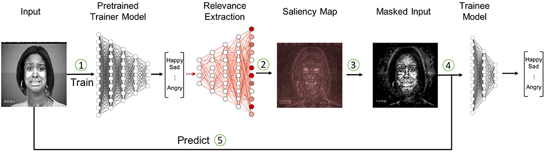
Figure 1. The relevance based masking process. (1) The input picture is classified by the Trainer network. (2) The decision is then analyzed via deep Taylor decomposition. (3) Based on the resulting saliency maps we generate masks that are zeroing out non-relevant information. (4) Masked images are used to train the Trainee network. (5) Predictions are always performed on the unmodified image. (Images are taken from the CKPlus dataset ©Jeffrey Cohn).

The motivation behind this approach is that we aim to improve the training of the new model by directing its focus toward relevant areas based on the knowledge of the Trainer network. This was inspired by the human learning process which occurs for instance when a teacher explains to a student which characteristics are relevant to determine a certain plant or animal species. We achieve this by masking the input data of the Trainee model during the training process so that it learns which areas are important. Afterwards, we validate the model with the unmasked input images to ensure that it has learned to identify the relevant areas by itself and can be used for predictions without requiring the additional masking step.

4. Datasets

While the proposed method is in general universally applicable, we test the validity of our approach for the task of facial expression recognition (FER). FER has been an active area of research for quite some time now and a lot of work has gone into the development of suitable datasets. However, those corpora vary greatly in terms of size, image- and label-quality. We therefore chose three different corpora for different purposes within our experimental setup. We use AffectNet to train the Trainer model because it is, to our knowledge, the largest available dataset for facial expression recognition tasks. This helps us to train a rather deep and therefore complex neural network. The CK+ dataset is used to compare the Trainer model to the human gaze annotations, since we wanted to test our model on images from a domain that the model has not seen before. Also, the comparably small size of the dataset allowed us to annotate the complete corpus. Finally, we use the FERPlus dataset to evaluate our system, since this corpus is large enough to obtain statistically relevant results.

In the following, we present those datasets in detail and briefly discuss their respective advantages for the employed tasks.

4.1. AffectNet

To train deep neural networks that learn an appropriate representation from raw sensory input, large amounts of annotated data are required. For the task of affect recognition, AffectNet (Mollahosseini et al., 2017) is one of the largest datasets available. The data from AffectNet has been collected by querying different search engines with a large amount of emotion related keywords. The so collected data has been manually annotated by specifically trained annotators with respect to both discrete categorical (Neutral, Happy, Sad, Surprise, Fear, Disgust, Anger, Contempt, None, Uncertain, Non-Face) and continuous dimensional (valence, arousal) emotions.

Overall, the corpus consists of around 420,000 annotated images. However, during our examination of the data, we identified 22,198 unique images that occur repeatedly with different labels assigned. For our experiments, we randomly chose one of these images each and removed the other duplicates. This way we reduced the size of the corpus by ~34,000 samples. Furthermore, we excluded all images with no annotated emotions, where the annotator was uncertain or where no faces were visible at all. This leaves us with 269,118 samples. For training and validation we kept the set-distribution provided by the authors. Since the official test-set has not been released yet, we use the validation set instead as suggested by Mollahosseini et al. (2017).

4.2. FERPlus

The FER-Dataset (Goodfellow et al., 2013), originally created by Pierre Luc Carier and Aaron Courvill, was gathered by crawling the internet with specific search queries. Over 600 search queries, consisting of a combination of emotion, gender, age, and ethnicity related keywords, have been created for this task. The first 1,000 pictures for each query have then been selected and filtered by human annotators. The remaining 35,887 images were then mapped onto seven distinct emotion categories (Anger, Disgust, Fear, Happiness, Sadness, Surprise, and Neutral). While this process enabled the creation of a relatively large corpus, the resulting labels are not very accurate. To improve the label accuracy of the FER dataset, Barsoum et al. (2016) decided to re-label the corpus, utilizing a different annotation process.

For this purpose they utilized crowd-sourcing to label each image by 10 different annotators with respect to the same eight categorical emotions, that already have been used in the AffectNet dataset as well as the categories unknown and not a face. The resulting dataset was called FERPlus. For our experiments with FERPlus we used a majority vote mechanism to determine the gold standard label for all annotations. After removing all images with unknown emotions or without faces, 35,488 images remained from the original training, validation and test sets. We kept the set-assignment as suggested by the authors of the dataset.

4.3. CKPlus

The Cohn-Kanade (CK) database by Kanade et al. (2000) has been specifically developed to serve as a comprehensive test-bed for comparative studies of facial expression analysis. To this end the authors recorded 210 adults across varying genders, ethnicity, and age groups. All participants were instructed to perform a series of facial expressions consisting of single action units or combinations of them. Each recording starts with a neutral facial expression and ends at the peak of the target facial expression. The last frame has then been annotated for facial action units (Ekman and Friesen, 1978).

Later the dataset was reprocessed and extended by Lucey et al. (2010) to overcome limitations that have become apparent since the original release. Besides adding more data to the corpus an important contribution of this reprocessing is the revising and validating of the emotion labels. This validation consisted of an elaborated multi step selection process that included the matching of the observed action units with the labeled emotion as well as visual inspection by emotion researchers. For our experiments we took the last image of each sequence as the emotion-labeled sample for the respective recording. For each session we also took the first image as a sample for the neutral class. Overall this leaves us with 654 images.

5. Implementation and Experiments

In this section we describe our implementations of the generic process we introduced in section 3. In the first subsection, we develop our Trainer model. After that, we present our approach to the creation of saliency maps and compare those maps the human perception in the third section. In the fourth and fifth section, we present three masking algorithms and describe how we use them to transfer knowledge from the Trainer to the Trainee model. Finally, we outline the measures we took to make our experiments deterministic.

5.1. Training the Trainer

To explore a suitable network architecture for our Trainer model, we trained a set of multiple state-of-the art CNNs from scratch on the previously described AffectNet dataset. Specifically, we selected four popular CNN-Architectures for our experiments: Xception (Chollet, 2017), MobileNetV2 (Sandler et al., 2018), InceptionV3 (Szegedy et al., 2016), and VGG-Face (Parkhi et al., 2015). All networks were trained until a plateau was reached using the same hyper-parameters. Specifically we used the Adam optimizer with a 0.001 learning rate, set the batch size to 32 and applied the categorical cross-entropy loss function to train the model.

For all models, we applied the same set of empirically evaluated data augmentation steps in order to increase the robustness and to prevent the models from learning position-dependent features: Each image has been rotated randomly up to 25 degrees and shifted randomly by up to 10 percent of its total width and height along the x-axis and the y-axis respectively. We also applied a random zoom of up to 85 percent of the original image dimensions. Furthermore, each color channel was shifted within a range of 20 percent and the overall brightness of the images was adjusted between 50 and 150 percent of the original values. Finally, we randomly flipped each input horizontally. To counter the heavily imbalanced sample distribution of the dataset (see Figure 2) we also applied a weighted loss function which weights each classes by their relative proportion in the training dataset. This approach has been suggested by Mollahosseini et al. (2017).

FIGURE 2

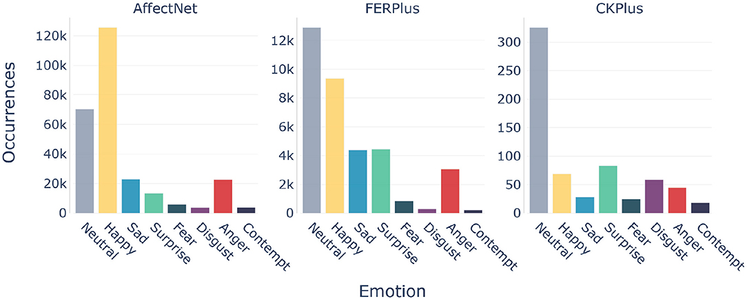
Figure 2. Distribution of emotion labels for all corpora after preprocessing.

After all models had been trained, we calculated the respective F1 scores on the validation set for each epoch and chose the overall best performing model as our Trainer model. In our experiments, the peak performance was reached by the InceptionV3 network architecture, trained for 42 epochs. This configuration achieved an F1-Score of 0.59, which is comparable to the proposed baseline of 0.58 on the validation set ¹.

However, before we employ our model as a Trainer we first want to analyze its strengths and weaknesses. Figure 3 shows the confusion matrix for the Trainer model. We can observe that on the one hand our model works best for samples of the Happy and Sad categories. On the other hand it does not perform well on the Neutral class which is often mistaken for Sad or Contempt. One possible explanation for this could be that the expressions within these classes look very similar and depend on the context for correct identification. Despite these shortcomings our model still performed rather well, considering that emotion recognition is a non-trivial task where even the agreement amongst human raters is often quite low (Goodfellow et al., 2013; Mollahosseini et al., 2017). An example for this can be seen on a subset of the AffectNet dataset, where the inter-rater agreement of two annotators was measured on 36,000 randomly selected samples. The results reported by the authors show that the highest agreement between those annotators exists for the happy class with 79.6%, while the least agreement is in the neutral class with 50.8%. The similarity in trends between the predictions of our model and the human inter-rater agreement suggests that our model is paying attention to similar regions of the input as the human annotators, when assessing the facial expression of a person while labeling the dataset.

FIGURE 3

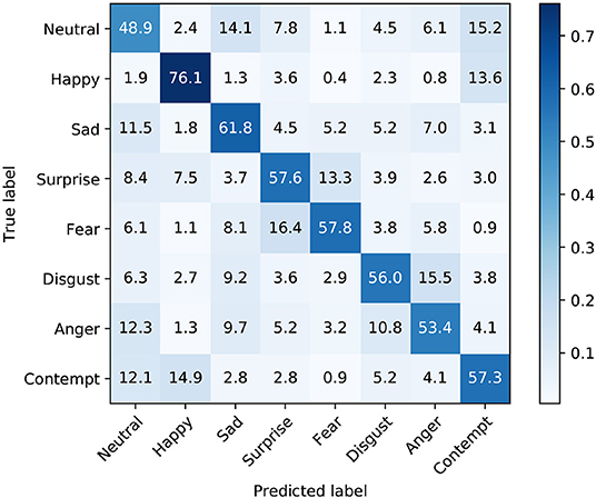
Figure 3. Confusion Matrix of the validation set of the AffectNet dataset using the InceptionV3 model.

5.2. Extracting Relevance

After training and selecting our Trainer model we then use it to calculate so called saliency maps from the research field of Explainable Artificial Intelligence (XAI), which aims to increase the explainability of incomprehensible models, such as neural networks. In general, saliency maps are heatmaps that highlight the parts of the input that were relevant for a particular decision and are the most commonly used method to explain the decision of neural networks visually (Adadi and Berrada, 2018). Currently, there are three popular ways to create such saliency maps. The first one relies on approximating the decision making process of an opaque model with a better explainable statistical model. Such an approach has been presented by Ribeiro et al. (2016) in the form of the LIME framework. While this method has the advantage of being model-agnostic, since the approximation only relies on the deviation in the prediction with respect to a change in the respective input, the inner workings of the classification algorithm are completely disregarded. The second method to create saliency maps for neural networks makes use of gradients to determine what parts of the input would change the prediction the most if they were slightly different (Simonyan et al., 2013).

In this work, we rely on the Layer-wise Relevance Propagation (LRP) concept by Bach et al. (2015). LRP utilizes the learned weights of a network to approximate the contribution of each input to the output by assigning a relevance value $R_i^l$ to every neuron $x_i^l$ of each layer l. The relevance value of the output neuron, which one wants to analyze, is set to be the output value of that neuron and this relevance value is then successively propagated backwards to each previous layer until it reaches the input layer where the neurons correspond to the input pixels. For our experiments we chose the LRP concept since, in contrast to the other two approaches, it satisfies the conservation property. This property states that the relevance values of the input $R_i^{input}$ sum up to the output of the neuron that one analyzes. Therefore, all relevance values are in proportion to each other, e.g., if a pixel's relevance value is twice as high as the relevance value of another pixel then it contributed twice as much to the prediction. This enables us to easily compare the contribution of different pixels and to choose the most relevant ones for our masking algorithms.

At each step of the relevance propagation, we use the deep Taylor decomposition approach introduced by Montavon et al. (2017) that aims to embed the LRP method into a more general theoretic framework by using a Taylor approximation to approximate how relevant each neuron $x_i^l$ of layer l was for the neurons $x_j^{l+1}$ of the subsequent layer l + 1. For this approximation, the relevance of $x_j^{l+1}$ needs to be modeled as a function $R_j^{l+1}(x^l)$ which depends on the neurons $x_i^l$ of the previous layer. This is typically done during previous steps of the relevance propagation. After such a function is found, one can decompose it using the Taylor series

$\begin{array}{ll}{R}_j^{l+1}(x^l)=R_j^{l+1}({\tilde{x}}^l)+{\displaystyle \sum _i\frac{\partial R_j^{l+1}}{\partial x_i^l}}{|}_{{\tilde{x}}^l}(x_i^l-{\tilde{x}}_i^l)+\epsilon ,& (1)\end{array}$

with Taylor residual ε and base point ${\tilde{x}}^l$. If the base point, which is chosen depending on $x_j^{l+1}$, is a root of $R_j^{l+1}$ and if one assumes that ε is small enough then the propagated relevance from $x_j^{l+1}$ to $x_i^l$ is given by

$\begin{array}{ll}\frac{\partial R_j^{l+1}}{\partial x_i^l}{|}_{{\tilde{x}}^l}(x_i^l-{\tilde{x}}_i^l).& (2)\end{array}$

This whole process is shown in Figure 4. Depending on the choice of base point ${\tilde{x}}^l$ we obtain different deep Taylor methods and many older LRP variants can be obtained in this way. For our study we use the deep Taylor implementation of the iNNvestigate framework by Alber et al. (2018). To give an impression about how the resulting saliency maps look like in our use case, Figure 5 depicts saliency maps that were generated to analyze our Trainer model when classifying samples of each AffectNet dataset class.

FIGURE 4

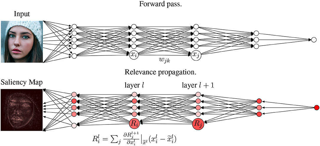
Figure 4. Visualization of the deep Taylor decomposition algorithm. After the forward pass, the output is propagated backward through the network to calculate relevance $R_i^l$ of each neuron i of every layer l for the prediction.

FIGURE 5

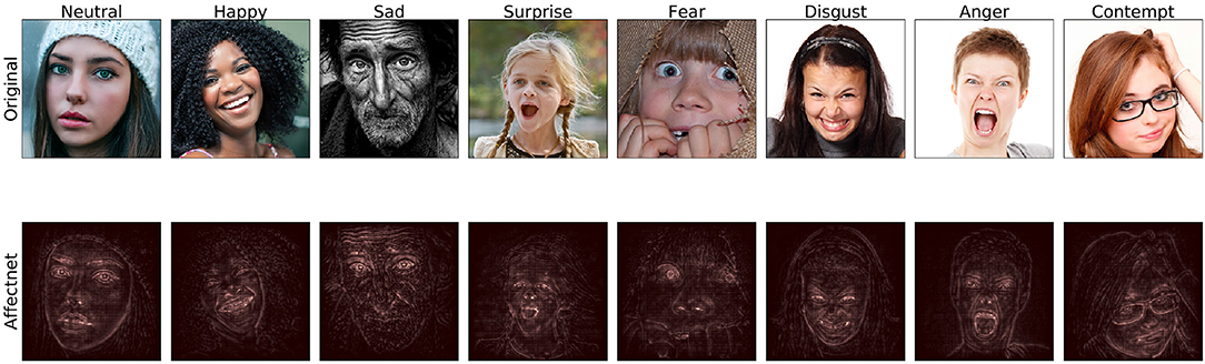
Figure 5. Saliency maps for samples of each class generated by applying deep Taylor decomposition to our Trainer model fitted to the AffectNet corpus.

5.3. Analyzing Human Perception

For our approach we are taking inspiration from the human gaze behavior. The idea behind this method is to only consider those regions as relevant, which were viewed by a human during the process of annotating the images. However, since obtaining the gaze information for large datasets like AffectNet or FERPlus is not feasible within a reasonable amount of time, we propose to use the model-generated saliency maps as proxy for the human attention. We consider this to be feasible because we assume that the most relevant areas for the model are similar to the regions considered by humans. In order to validate this assumption, we conducted a preliminary study in which we tracked the eye movements of human annotators during the labeling process and compared their gaze behavior with the previously created saliency maps.

5.3.1. Method

Two human annotators participated in the experiment. Both have not received special training for this task, but are experienced in labeling emotion related corpora. The participants were instructed to label the complete CKPlus dataset with respect to the eight discrete categorical classes of the original labeling scheme. The CKPlus dataset was specifically chosen since it is well-established in the community as a corpus for research into detecting individual facial expressions. The participants were seated 70 cm in front of a 27” monitor running at 2560 x 1440 pixel resolution. A The Eye Tribe ET1000 eye tracker was positioned beneath the monitor to record the eye movements of the annotators during the process. The participants then started the labeling process using a custom written interface. A GUI displayed images from the dataset in random order for the annotators to label. All images were displayed in 1200 x 1200 pixel square in the center of the display. Once they decided on a label, the participants could then just speak the respective label into a microphone. This way we avoided introducing additional noise into the eye tracking recordings since the participants gaze could always remain focused on the user interface. No time constraints were imposed on the labeling process. By pressing a key on the keyboard in front of the participants, they could themselves determine when the next image was displayed. Between each image a blank screen was displayed for 500 ms. After the blank screen, a central fixation cross appeared for 200 ms followed by another blank screen for 500 ms. This process was adopted from Utz and Carbon (2016).

5.3.2. Evaluation

A popular method for investigating a user's gaze behavior is the visualization via heatmaps (Courtemanche et al., 2018). While heatmaps can be used to create graphical representations for various types of input data, the processing of eye tracking data needs some additional consideration. The main types of human eye movement to consider are fixations and saccades. Fixations can be viewed as maintaining the visual gaze on a target in order to obtain information while saccades are rapid movements between fixations. Since conscious fixations occur, for example, when reading a text or viewing an image, they are commonly used as data points to create heatmaps, while saccades are often ignored. The human field of view (FOV) consists of three concentric areas of decreasing acuity around the currently fixated gaze point: The foveal-, parafoveal-, and peripheral area. Usually, the eye moves in a way that places visual points of interest within the foveal area, where the acuity is the largest. But while the image becomes more blurred toward the edges of the visual field, the sensory input from the parafoveal and peripheral can still be processed to extract useful information (Courtemanche et al., 2018). Figure 6 illustrates the different areas in the visual field for a given fixation.

FIGURE 6

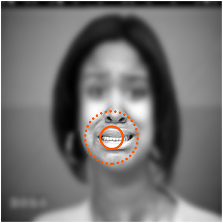
Figure 6. Illustrated visual perception of human gaze for the displayed image during the annotation. The inner ring shows the foveal area, the dashed ring encircles the parafoveal area and the rest corresponds to the peripheral vision. The sharpness of the perceived image is decreasing from the center of the foveal area to the outside. (Images are taken from the CKPlus dataset ©Jeffrey Cohn).

The maximum distance from a fixation point where the user might cognitively observe objects is called visual span and is determined by the visual angle and the distance to the viewing plane. To generate informative heatmaps for eye tracking behavior, Blignaut (2010) suggest using a visual angle of 5°. This results in an observed area that is equivalent to the parafoveal area. The distance to the viewing plane is the distance of the user to the monitor.

Similar to the heatmap creation procedure described by Courtemanche et al. (2018), we calculate each point for the heatmap as follows:

$\begin{array}{l}I(x,y)={\displaystyle \sum _{n=0}^N}p(x,y,f_n)\end{array}$

The intensity I of a given pixel with coordinates x and y in the heatmap is defined by the sum over the probabilities p for each fixation f_n that the pixel has been perceived by the user during the time of the fixation. To estimate this probability we apply a Gaussian scaling function,

$\begin{array}{l}p(x,y,f_n)=e^{\frac{-({(x-f_{n,x})}^2+{(y-f_{n,y})}^2)}{2c^2}}.\end{array}$

where x and y are the pixel coordinates of the heatmap and f_{n, x} and f_{n, y} are the coordinates of the fixation f_n. The constant c can be arbitrarily chosen, but is related to the full width at half maximum (FWHM) of p which is given by:

$\begin{array}{l}FWHM=2.358·c\end{array}$

Blignaut (2010) suggested to choose c as such that FWHM is equal to 40% of the visual span. We therefore set c to

$\begin{array}{l}c=0.17·visualspan.\end{array}$

To compare the eye gaze heatmaps with the saliency maps of our model, we apply the same heatmapping algorithm to the raw relevance values calculated by the deep Taylor decomposition approach described in section 5.2. To limit the visual focus of the network, we only consider the n most relevant pixels for this task, where n is equal to the average number of fixated points by both of our participants during the eye tracking recordings. Besides a visual inspection, we also generated masks from the contour of the heatmaps to quantitatively compare the overall focused area. To this end, we calculate the ratio of the overlapping area from the user- and model-generated heatmap to the pixel-wise union of both areas. The result of this metric is a value between 0 and 1. A value of 1 means that both heatmaps have identical position and contour, while a value of 0 means that there is no overlap between the viewed areas at all.

The results are displayed in Table 1. When comparing the overlapping areas between the heatmaps of each user and the model, we can see that they approximately share 40% of the pixels. Similarly, the values for the Spearman correlation and the Cosine Distance metric indicate a medium accordance between them. While the perceived areas shown in Figure 7 might have different contours, both of them contain the most relevant areas, such as the eyes, nose, and mouth. We can see that the regions that are considered relevant in this case are similar to areas at which the human annotators looked during the labeling process.

TABLE 1

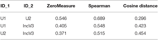
Table 1. Comparison of the overall perceived areas between two annotators and the respectively generated heatmaps of our explanatory model.

FIGURE 7

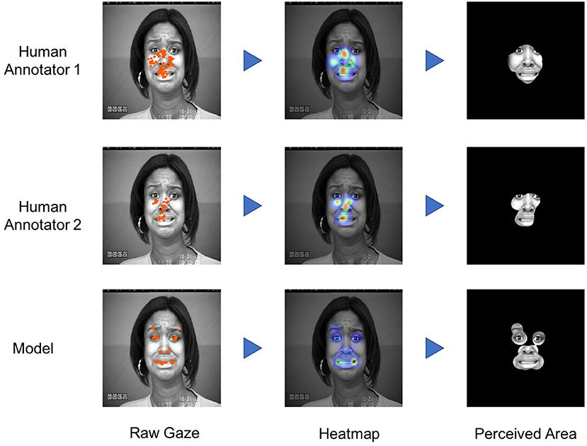
Figure 7. Eyegaze comparison between two users, during the annotation of an image, with the respective areas that were relevant for our neural network to classify this image. (Best viewed in color. Images are taken from the CKPlus dataset ©Jeffrey Cohn).

5.4. Masking the Input

To create masked versions of a dataset we first need to figure out what the most relevant regions are for each input image. While the concept “most relevant” can be easily grasped by humans by just looking at the saliency map (see Figure 4), it is difficult to find a generic algorithm that selects exactly those regions. When creating a saliency map for the prediction of a specific input every part of this input gets a specific relevance value assigned. Higher values imply that the input has been more relevant for the decision of the model while lower values are indicating that the input has been less relevant, those terms are purely relative. It is not obvious at what value information can actually be considered as not important for the prediction of the Trainer and should therefore be zeroed out in the masking process. In this section we are therefore addressing the question “How relevant is actually relevant?”

To this end we implemented and tested three different masking algorithms that zero out parts of an input picture based on the saliency map, for this picture, of the Trainer network. Two of those algorithms build up on previous work in Schiller et al. (2019) and the third is inspired by the human perception we investigated in section 5.3. Each of those algorithms takes an image I and generates a binary mask M with same shape as the input image. The masked image is then created by taking the component wise product I * M.

The first masking algorithm we tested is negative masking, where we are zeroing out the top 10 percent of all relevance values. That is each entry m_i of the mask M is calculated based on the corresponding relevance values R_i of the saliency map as

$\begin{array}{l}{m}_i:=\{\begin{array}{ll}0\hfill & \text{if }{R}_i\text{ is part of the top 10\% of all }{R}_i’\text{s}\hfill \\ 1\hfill & \text{if not.}\hfill \end{array}\end{array}$

The motivation behind this algorithm was to force the Trainee network to pay attention to features that were not used by the Trainer network. The resulting Trainee model could then be used in a fusion system together with the Trainer network.

The second masking algorithm we implemented is mean masking which zeroes out all pixels whose relevance values R_i are smaller than the mean relevance value of the image. In this case m_i is calculated by

$\begin{array}{l}{m}_i:=\{\begin{array}{ll}1\hfill & \text{if }{R}_i\ge \frac{{\displaystyle {\sum }_{i=1}^N{R}_i}}{N}\hfill \\ 0\hfill & \text{if not},\hfill \end{array}\end{array}$

where N is the total number of pixels in the input picture. This masking aims to accelerate the training process of the Trainee network by only showing the areas of an input picture that were already identified as relevant for the Trainer network.

For the final masking algorithm we choose the n pixels with the highest relevance values, where n is the average number of fixated points by the participants in our eye tracking study described in section 5.3. We then use those pixels as replacement for human fixations and apply the heatmapping approach presented in section 5.3 to identify relevant information in an input image. Based on this heatmap we generate a mask by setting m_i to zero if the intensity I_i of the heatmap at the corresponding pixel i is also zero. In total m_i is calculated by

$\begin{array}{l}{m}_i:=\{\begin{array}{ll}1\hfill & \text{if }{I}_i>0\hfill \\ 0\hfill & \text{if not.}\hfill \end{array}\end{array}$

Since this form of masking is modeled after the human perception, we refer to it as perceptive masking.

Figure 8 shows an example of all masking approaches. Overall, the negative masking method still retains most of the original input image since only 10 percent of the pixels are masked out. In contrast to that, the perceptive masking removes the majority of the image and only leaves the most important areas such as the eyes, nose, and mouth visible. Compared to the other two methods, the mean masking approach provides a middle ground where the lesser relevant half of all pixels are removed.

FIGURE 8

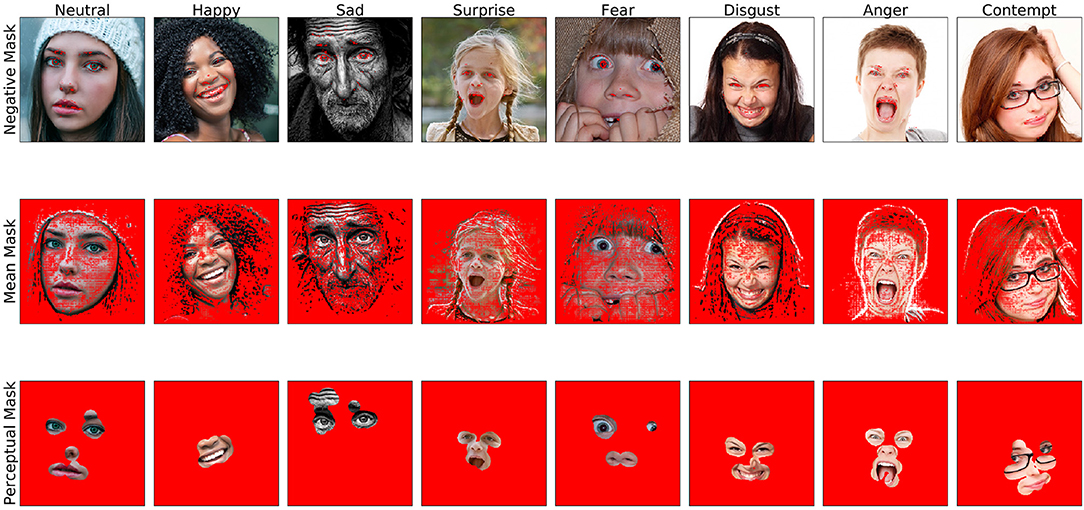
Figure 8. Illustration of the masking algorithms used for training. (1) The first row shows the negative masks where the most relevant regions are zeroed out. (2) The middle row displays masked images, using mean masking where pixels with less than average relevance values were zeroed out. (3) Finally the third mask uses a perceptive masking algorithm, that is modeled after the human eyegaze behavior. The masked areas in these images are highlighted in red color to improve visibility (Best viewed in color).

5.5. Training the Trainee

In our experimental setup we employed the InceptionV3 architecture with ~23.8 million parameters trained on the AffectNet dataset as Trainer model (see section 5.1). As the Trainee we chose the MobileNetV2 architecture which only has 3.5 million parameters and is therefore more lightweight and can be trained faster than the original Trainer model. The reason why we chose these architectures is because we wanted to show that our approach can be used to transfer the knowledge from a much larger network with almost seven-times as many parameters to a small and lightweight model with a completely different architecture which enables new application scenarios for the Trainee network (e.g., devices with limited computational capabilities like mobile phones).

As classification target for the Trainee network we chose the FERPlus dataset for the task of facial expression recognition. While transfer learning is most often performed by transferring knowledge from related tasks with more data available, we specifically chose to train our Trainee model for the same task as the Trainer model. Applying the perceptive masking algorithm our model serves as proxy for a human annotator. This way we aim to assess the validity of directly integrating the attention of a human annotator into the system in the future.

To establish a baseline we first trained our model on the non-masked FERPlus data, without using any transfer learning.

To evaluate our transfer learning approach proposed in section 3, we created a masked version of the FERPlus dataset for each masking algorithm introduced in section 5.4: negative-, mean-, and perceptive-masking. For this we used each image I of the FERPlus corpus as input for our Trainer model and generated a saliency map that analyzes the prediction of our Trainer model for this input I. Based on these saliency maps we generated binary masks M with the same shape as the input picture and then used the masked image, which is the componentwise product I*M, as new training image. In this way we encode knowledge from the Trainer network in the new training set by guiding the attention to certain areas, depending on the saliency maps of the Trainer model and the chosen masking algorithm.

This leaves us with three new versions of the FERPlus dataset. By training the Trainee network on one of those masked training set we can transfer knowledge from the Trainer network to a completely new model architecture instead of having to use the same architecture with pretrained weights as in traditional transfer learning approaches. This enables us to experiment with and compare different architectures for the Trainee network.

In addition to training the Trainee model exclusively on masked training data, we also trained a version of our Trainee model for each masking algorithm, where we first used the masked training set and then switch to the original non-masked dataset after a few epochs. After that, the unmodified images are used as input to make sure that the specifics of the new corpus are taken into account.

In section 6 we present a comparison of the training progress of our seven different Trainee models.

5.6. A Word on Reproducibility

For the evaluation of our proposed approach we used TensorFlow² to implement the necessary experiments and performed the model training on NVIDIA Tesla V100 GPUs. However, during training we noticed that the initial results were not deterministic and could not be reproduced in consecutive runs even though the parameters were not changed and the random seeds were fixed. Figure 9 shows the progression of three identical runs which resulted in different slopes for the F1 and Loss metrics. As illustrated, the indeterministic influence factor led to massive differences between each learning curve and caused that in one case our model started learning after 3.5 million steps while in the other case it already began after 0.8 million steps. Additionally, we occasionally observed runs where our model immediately started overfitting or did not learn anything at all even though the configuration was the same. We suppose that, since most runs eventually ended up at similar performance levels after enough training time this was not as apparent or relevant in previous research, but because one of our goals was to improve the learning process and thus the initial model performance we needed to be able to create reliable and reproducible learning curves in order to compare them to each other. This problem has recently been acknowledged by NVIDIA at the GPU Technology Conference 2019 where they reported similar observations and discussed their work to eliminate non-determinism from deep learning when using TensorFlow on GPUs (Riach, 2019).

FIGURE 9

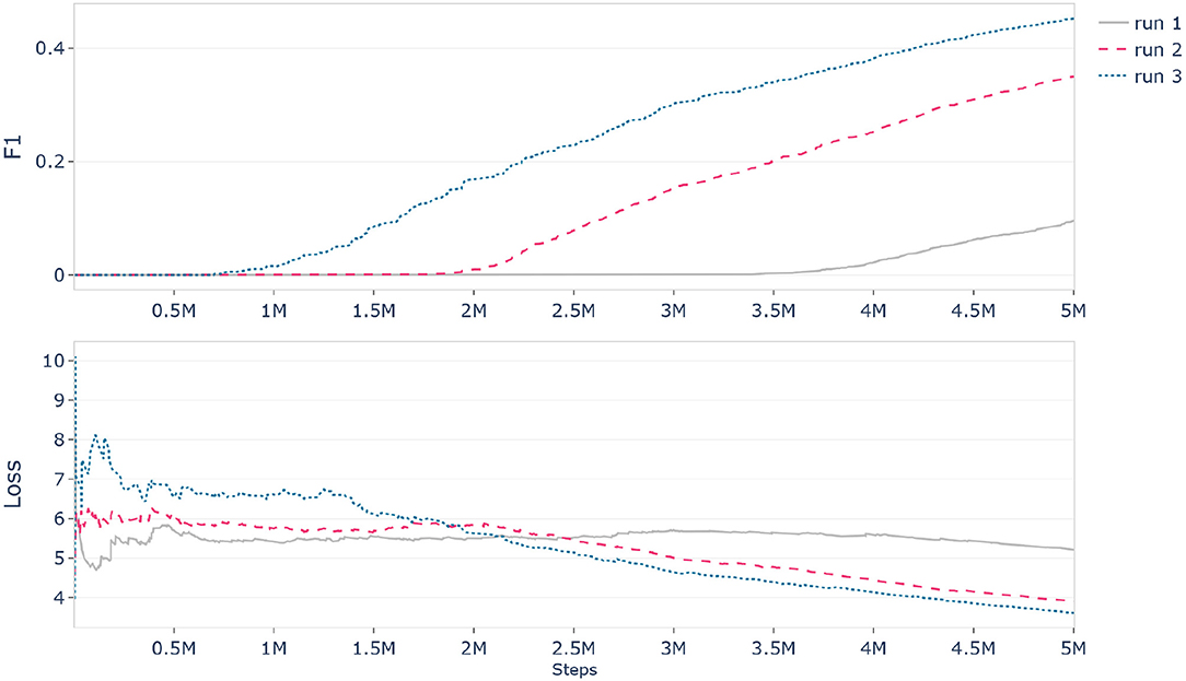
Figure 9. History of F1 and Loss metrics for three identical training runs of the same model with the same configuration and the same random seeds which produced indeterministic results before applying changes to ensure reproducibility.

After extensive research and testing we found two solutions to solve this problem. The first one was to perform all experiments on the CPU instead of the GPU, but since this would have required much more computation time we decided to use an alternative solution. For that, we set up an NVIDIA Docker environment³ and used the official TensorFlow container⁴ provided by NVIDIA. Since version 19.06 this container includes a determinism feature which can be enabled to ensure the selection of deterministic convolution and max-pooling algorithms as well as the deterministic operation of bias additions on GPUs. In addition to that, the number of worker threads had to be limited to one, since parallel processing across multiple threads can also introduce unreliable behavior and thus lead to indeterministic results. After applying all of these changes we were finally able to reproduce the exact progression of each metric across multiple consecutive runs with the same configuration.

6. Results and Discussion

In this section, we present and discuss the results of our experiments, comparing the training progress of different implementations of the generic transfer learning approach proposed in section 3. To this end, we utilized our InceptionV3 model which was pretrained on the AffectNet dataset (section 5.1) to mask the FERPlus dataset with the algorithms introduced in section 5.4 and subsequently train a MobileNetV2 architecture network on the modified data (section 5.5).

Figure 10 shows the learning curves of our Trainee model for each of our masking algorithms, as well as the "no mask" base model which is trained on the unmasked, full images. As illustrated, the mean masking algorithm greatly accelerated the training process in the beginning, but fell under the performance of the network trained on plain images after about 700,000 training steps. This is to be expected since the masking process hides information from the network. While this helps the network to process the remaining relevant input the additional information would still be useful to achieve an overall better performance.

FIGURE 10

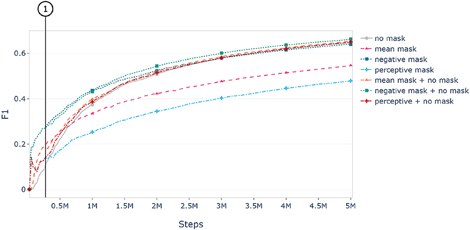
Figure 10. Learning curves of the Trainee network trained on differently masked versions of the Ferplus dataset. Here, “no mask” refers to a model, that has been trained on the full, unmasked images. The combined version (e.g., “mean mask + no mask”) have been trained on the masked corpus for 9 epochs (marked by ①) before switching to the unmodified dataset. The shown results are evaluated on the unmodified images of the validation set.

Additionally, Figure 10 shows that switching from the masked input data to the unmasked input during training after nine epochs retains the initial acceleration of the masking algorithm while obtaining slightly higher performance than when just training with the input image directly.

Since the performance of the Trainer model is skewed toward the happy class (see Figure 3), we investigate whether our transfer-learning approach introduces the same bias to the Trainee model. To this end we calculate the confusion matrices for our best performing model, as well as the “no mask” base model, to compare the per-class-performance between them. Figure 11 shows the confusion matrix for the “no mask” base model. Our best performing model, trained first on the negative masked images and subsequently on the full, unmasked input is shown in Figure 12. Each model has been trained for five million steps on the training set of the FERPlus dataset. The official validation set of the corpus has been used for validation.

FIGURE 11

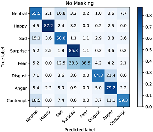
Figure 11. Confusion Matrix of the validation set of the FERPlus dataset using the reference baseline model. The model has been trained on the unmasked images for five million steps.

FIGURE 12

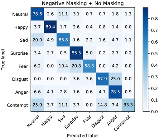
Figure 12. Confusion Matrix of the validation set of the FERPlus dataset using the best performing model. The model has been trained on the negative masked images as well as the unmasked input for five million steps.

Comparing the two matrices, we find that the biggest difference in per class performance lies in the prediction quality of fear and contempt. While the base model struggles to predict fear correctly, the masked model exhibits a similar weakness with the contempt class. However, since the trainer model does not show a skew toward either of those classes, we argue that this phenomenon is not due to the bias of the Trainer model.

Initially, we intended to use the negative masking algorithm to zero out relevant information and therefore train a network that focuses on different areas than the original Trainer network. This newly created network could then be fused on the decision level with the explanatory network to improve results—an approach that has been successfully used before in a different domain (Schiller et al., 2019). Yet we found that the negative masking approach performed better than the mean masking method. A potential reason for this contra-intuitive observation lies in the fact that the zeroing out of the most important pixels might have acted as a highlighting and helped the network to learn rough shapes of important features, such as the eyes or the mouth (see Figure 8).

The third approach we tested was the implementation of perceptive masking which is modeled after the human gaze behavior. We found that the perceptive masking approach performed the worst if we do not switch to unmasked training images. When switching the input after nine epochs to the unmodified images, the performance was comparable with the mean masking approach. Most likely this is due to the additional loss in information caused by the more restrictive masking process. This is related to the fact that the deep Taylor decomposition we used for saliency map creation assess the relevance of every pixel of the input image. It is therefore necessary to choose the most relevant pixels as proxy for human fixations. More selective saliency map generation algorithms like the ones in Huber et al. (2019) or Mopuri et al. (2018) might be better suited for this particular masking algorithm, since they already select a smaller number of pixels.

If possible we think that perceptive masking should be used with actual human fixations. This has the additional advantage of incorporating human knowledge into the training loop. While the similarity measurements and the visual inspection of the perceived areas in section 5.3 indicate that our Trainer model is overall looking at similar facial features as the human annotators (eyes, mouth, nose, etc.), a closer look reveals that it does not necessarily focus on the correct features for a specific prediction. An example for this can be seen in Figure 13 that depicts a case where the Trainer model predicted an image wrongly as anger. The gold standard label of the image is disgust which is indicated by a wrinkled nose or the raising of the upper lip (Lucey et al., 2010). Here the model is clearly ignoring the nose wrinkles and focuses on the mouth, nose, and eyes instead. In contrast, the human annotator is mainly paying attention to the wrinkled nose which is highly relevant for the prediction.

FIGURE 13

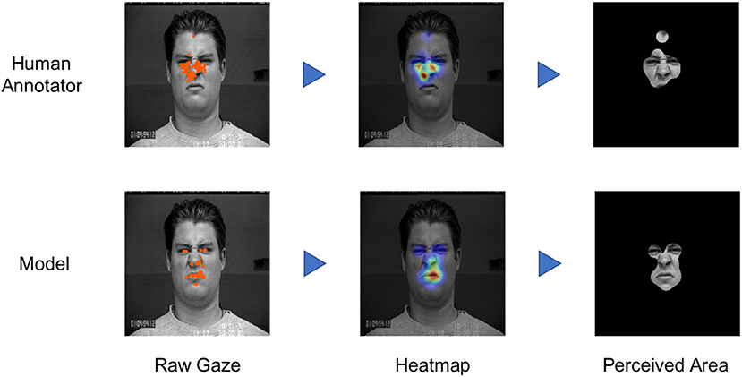
Figure 13. Example for an image that got correctly labeled as disgust by the human annotator but not by our Trainer model. Comparing the gaze behavior of the human with the most relevant pixels for the decision of our Trainer model shows that our model is not focusing on the characteristic nose wrinkles (Best viewed in color. Images are taken from the CKPlus dataset ©Jeffrey Cohn).

In general, we observed that our approach can contribute to a faster training in all cases. However, the masking should be discarded after an initial warm-start to maintain pace and ensure the overall quality of the model.

One advantage of our proposed transfer learning process is that it is explainable in the sense that we can see what kind of information is transferred from the Trainer to the Trainee model by looking at the generated saliency maps or masked images. This potentially enables us to recognize whether the transferred information stems from faulty reasoning of the Trainer network. In this case, one should remove the faulty samples from the masked training set or use another Trainer model.

In contrast to traditional transfer learning approaches, like fine-tuning, our proposed method does not incorporate the source model into the architecture of the target model. We refer to this effect as being model-agnostic. Being model-agnostic comes with three major advantages. First of all, the new Trainee network does not need to use pretrained weights from the Trainer network and therefore we are free to choose any kind of architecture for the Trainee network without retraining the Trainer model. Secondly, the transfer of relevant regions via the augmentation of the input data has the advantage of being independent of the Trainer model acting as source of knowledge. The only condition is that it is possible to create saliency maps for the predictions of the Trainer model. This way our approach is not restricted to the use of neural networks. In theory, one could use any model or even humans as source of knowledge, as long as it is possible to assign a relevance value to each input value in relation to a specific prediction. Thirdly, our approach is not limited to one Trainer model. It can be easily adapted to incorporate the trained knowledge from multiple sources.

Unlike traditional transfer learning approaches however, our method does not provide any information about the interrelations between the input pixels. Therefore the learned features, which are passed from one model to another when using the source model as feature extractor or for fine tuning, must be learned again in our scenario. Since we have shown that our Relevance-based Data Masking (RBDM) approach, in its current form, can achieve a positive impact on the training speed but does not contribute much to increase the overall performance of the Trainee model we think that the choice of transfer learning method depends on the intended application. If there is already a pretrained model available whose architecture fits the respective target use case then we recommend to go with the traditional feature extraction or fine tuning approach. On the other hand, if complete control over the architecture of the target model is a concern (e.g., to ensure inference performance or restrict deployment size), or knowledge from other sources should be integrated into the training process, we suggest to apply our proposed RBDM method.

7. Conclusion

In this work we proposed a method for facial expression recognition that utilizes saliency maps to transfer knowledge from an arbitrary source to a target network by essentially “hiding” non-relevant information. In contrast to common transfer learning approaches our proposed method is independent of the employed model, since the knowledge is solely transferred via an augmentation of the input data. This property comes to play when there is no pretrained model available whose architecture is appropriate for the respective application (e.g., when specific criteria for inference performance or model size must be met).

Furthermore, we conducted a preliminary eye tracking study to obtain information on the human attentional process for facial expression recognition. The goal of this study was to assess the feasibility of incorporating the human gaze behavior directly into our proposed method. We used the results of this study to develop an approach that combines the gained information with saliency mapping techniques to assess the regions of the input that are most relevant for the decision of a pretrained neural network. This way we were able to mimic the attentional focus of the human annotators for our pretrained model and could therefore integrate the model into our method as a human proxy. This allowed us to evaluate the benefits of integrating the human gaze behavior empirically on a larger dataset that would have been too expensive to label. However, we also found that while our model was overall considering the same set of facial features (e.g., nose, mouth, eyebrows, etc.) to recognize facial expressions as the human annotators, we found that it did not necessarily consider the most characteristic features for the respective predictions. This suggests that there might be additional benefits of using actual humans perception as source for our proposed transfer learning process.

Finally, we applied our approach to transfer knowledge between two domains and model architectures. To this end we used the InceptionV3 model architecture trained on the AffectNet dataset as the source, and the smaller MobileNetV2 architecture on the FERPlus dataset as the target model. The evaluation of our experiments showed that our new model was able to adapt to the new domain faster, when forced to focus on the parts of the input that were considered relevant by our source model. However, in order to not forfeit the overall performance we needed to switch the input to the full images after a few epochs of training.

Overall, we argue that our approach allows us to exploit saliency maps to transfer knowledge between models. In the future we would like to explore additional ways to utilize saliency maps for this task, for example by using them as additional training targets or combining our methods with other transfer learning approaches.

Data Availability Statement

The raw data supporting the conclusions of this article will be made available by the authors, without undue reservation, to any qualified researcher.

Author Contributions

The idea was conceived by TH and DS. DS managed the project, oversaw the development as well as the study and wrote major parts of the paper and code. TH and MD conducted experiments, wrote certain sections of the article and contributed major revisions to the paper. EA supervised the entire work as well as the drafting of the article. All authors contributed to manuscript revision, read, and approved the submitted version.

Funding

This work has been partially funded by the Deutsche Forschungsgemeinschaft (DFG) under project DEEP (Grant Number 392401413), by the German Federal Ministry of Education and Research (BMBF) under project EmmA (FKZ16SV8028) and by the Bavarian Ministry of Science and Arts (StMWK) under project ForDigitHealth.

Conflict of Interest

The authors declare that the research was conducted in the absence of any commercial or financial relationships that could be construed as a potential conflict of interest.

Footnotes

1. ^http://mohammadmahoor.com/affectnet/. Mollahosseini et al. (2017) proposed to use the validation set for the baseline approach since the test set has not been officially released.

2. ^https://tensorflow.org

3. ^https://github.com/NVIDIA/nvidia-docker

4. ^https://ngc.nvidia.com/catalog/containers/nvidia:tensorflow

References

Adadi, A., and Berrada, M. (2018). Peeking inside the black-box: a survey on explainable artificial intelligence (XAI). IEEE Access 6, 52138–52160. doi: 10.1109/ACCESS.2018.2870052

CrossRef Full Text | Google Scholar

Albanie, S., Nagrani, A., Vedaldi, A., and Zisserman, A. (2018). Emotion recognition in speech using cross-modal transfer in the wild. arXiv preprint arXiv:1808.05561. doi: 10.1145/3240508.3240578

CrossRef Full Text | Google Scholar

Alber, M., Lapuschkin, S., Seegerer, P., Hägele, M., Schütt, K. T., Montavon, G., et al. (2018). INNvestigate neural networks! arXiv preprint arXiv:1808.04260.

Google Scholar

Bach, S., Binder, A., Montavon, G., Klauschen, F., Müller, K.-R., and Samek, W. (2015). On pixel-wise explanations for non-linear classifier decisions by layer-wise relevance propagation. PLOS ONE 10:e0130140. doi: 10.1371/journal.pone.0130140

PubMed Abstract | CrossRef Full Text | Google Scholar

Barsoum, E., Zhang, C., Ferrer, C. C., and Zhang, Z. (2016). “Training deep networks for facial expression recognition with crowd-sourced label distribution,” in Proceedings of the 18th ACM International Conference on Multimodal Interaction (Tokyo: ACM), 279–283.

Google Scholar

Blignaut, P. (2010). “Visual span and other parameters for the generation of heatmaps,” in Proceedings of the 2010 Symposium on Eye-Tracking Research & Applications (Austin, TX: ACM), 125–128.

Google Scholar

Buciluǎ, C., Caruana, R., and Niculescu-Mizil, A. (2006). “Model compression,” in Proceedings of the 12th ACM SIGKDD International Conference on Knowledge Discovery and Data Mining (Philadelphia, PA: ACM), 535–541.

Google Scholar

Chollet, F. (2017). “Xception: Deep learning with depthwise separable convolutions,” in Proceedings of the IEEE Conference on Computer Vision and Pattern Recognition (Honolulu, HI), 1251–1258.

Google Scholar

Courtemanche, F., Léger, P.-M., Dufresne, A., Fredette, M., Labonté-LeMoyne, É., and Sénécal, S. (2018). Physiological heatmaps: a tool for visualizing users' emotional reactions. Multimedia Tools Appl. 77, 11547–11574. doi: 10.1007/s11042-017-5091-1

CrossRef Full Text | Google Scholar

Ekman, P., and Friesen, W. V. (1978). Manual of the facial action coding system (FACS). Palo Alto, CA: Consulting Psychologists Press.

Fernandez, P. D. M., Peña, F. A. G., Ren, T. I., and Cunha, A. (2019). Feratt: Facial expression recognition with attention net. arXiv preprint arXiv:1902.03284.

Google Scholar

Ge, S., Zhao, S., Li, C., and Li, J. (2018). Low-resolution face recognition in the wild via selective knowledge distillation. IEEE Trans. Image Process. 28, 2051–2062. doi: 10.1109/TIP.2018.2883743

CrossRef Full Text | Google Scholar

Goodfellow, I. J., Erhan, D., Carrier, P. L., Courville, A., Mirza, M., Hamner, B., et al. (2013). “Challenges in representation learning: a report on three machine learning contests,” in International Conference on Neural Information Processing (Daegu: Springer), 117–124.

Google Scholar

Green, M. J., and Phillips, M. L. (2004). Social threat perception and the evolution of paranoia. Neurosci. Biobehav. Rev. 28, 333–342. doi: 10.1016/j.neubiorev.2004.03.006

PubMed Abstract | CrossRef Full Text | Google Scholar

Huber, T., Schiller, D., and André, E. (2019). “Enhancing explainability of deep reinforcement learning through selective layer-wise relevance propagation,” in KI 2019: Advances in Artificial Intelligence - 42nd German Conference on AI (Kassel), 188–202.

Google Scholar

Itti, L., and Koch, C. (2001). Computational modelling of visual attention. Nat. Rev. Neurosci. 2, 194–203. doi: 10.1038/35058500

PubMed Abstract | CrossRef Full Text | Google Scholar

Kanade, T., Cohn, J. F., and Tian, Y. (2000). “Comprehensive database for facial expression analysis,” in Proceedings Fourth IEEE International Conference on Automatic Face and Gesture Recognition (Cat. No. PR00580) (Grenoble: IEEE), 46–53.

Google Scholar

Li, J., Seltzer, M. L., Wang, X., Zhao, R., and Gong, Y. (2017). Large-scale domain adaptation via teacher-student learning. arXiv preprint arXiv:1708.05466. doi: 10.21437/Interspeech.2017-519

CrossRef Full Text | Google Scholar

Li, Y., Zeng, J., Shan, S., and Chen, X. (2018). Occlusion aware facial expression recognition using cnn with attention mechanism. IEEE Trans. Image Process. 28, 2439–2450. doi: 10.1109/TIP.2018.2886767

CrossRef Full Text | Google Scholar

Lucey, P., Cohn, J. F., Kanade, T., Saragih, J., Ambadar, Z., and Matthews, I. (2010). “The extended cohn-kanade dataset (ck+): a complete dataset for action unit and emotion-specified expression,” in 2010 IEEE Computer Society Conference on Computer Vision and Pattern Recognition-Workshops (San Francisco, CA: IEEE), 94–101.

Google Scholar

Mac Aodha, O., Su, S., Chen, Y., Perona, P., and Yue, Y. (2018). “Teaching categories to human learners with visual explanations,” in Proceedings of the IEEE Conference on Computer Vision and Pattern Recognition (Salt Lake City, UT), 3820–3828.

Google Scholar

Meng, D., Peng, X., Wang, K., and Qiao, Y. (2019). “Frame attention networks for facial expression recognition in videos,” in 2019 IEEE International Conference on Image Processing (ICIP) (Taipei: IEEE), 3866–3870.

Google Scholar

Meng, Z., Li, J., Zhao, Y., and Gong, Y. (2019). “Conditional teacher-student learning,” in ICASSP 2019-2019 IEEE International Conference on Acoustics, Speech and Signal Processing (ICASSP) (Brighton: IEEE), 6445–6449.

Google Scholar

Minaee, S., and Abdolrashidi, A. (2019). Deep-emotion: facial expression recognition using attentional convolutional network. arXiv preprint arXiv:1902.01019.

Google Scholar

Mollahosseini, A., Hasani, B., and Mahoor, M. H. (2017). Affectnet: a database for facial expression, valence, and arousal computing in the wild. IEEE Trans. Affect. Comput. 10, 18–31. doi: 10.1109/TAFFC.2017.2740923

CrossRef Full Text | Google Scholar

Montavon, G., Lapuschkin, S., Binder, A., Samek, W., and Müller, K. (2017). Explaining nonlinear classification decisions with deep taylor decomposition. Pattern Recogn. 65, 211–222. doi: 10.1016/j.patcog.2016.11.008

CrossRef Full Text | Google Scholar

Mopuri, K. R., Garg, U., and Babu, R. V. (2018). Cnn fixations: an unraveling approach to visualize the discriminative image regions. IEEE Trans. Image Process. 28, 2116–2125. doi: 10.1109/TIP.2018.2881920

PubMed Abstract | CrossRef Full Text | Google Scholar

Ng, H.-W., Nguyen, V. D., Vonikakis, V., and Winkler, S. (2015). “Deep learning for emotion recognition on small datasets using transfer learning,” in Proceedings of the 2015 ACM on International Conference on Multimodal Interaction (Seattle, WA: ACM), 443–449.

Google Scholar

Parkhi, O. M., Vedaldi, A., Zisserman, A., et al. (2015). “Deep face recognition,” in bmvc, Vol. 1 (Swansea), 6.

Google Scholar

Riach, D. (2019). GTC Silicon Valley-2019 ID:S9911:Determinism in Deep Learning. Available online at: https://developer.nvidia.com/gtc/2019/video/S9911 (accessed October 1, 2019).

Google Scholar

Ribeiro, M. T., Singh, S., and Guestrin, C. (2016). “Why should i trust you?: explaining the predictions of any classifier,” in Proceedings of the 22nd ACM SIGKDD International Conference on Knowledge Discovery and Data Mining (San Francisco, CA: ACM), 1135–1144.

Google Scholar

Sandler, M., Howard, A., Zhu, M., Zhmoginov, A., and Chen, L.-C. (2018). “Mobilenetv2: inverted residuals and linear bottlenecks,” in Proceedings of the IEEE Conference on Computer Vision and Pattern Recognition (Salt Lake City, UT), 4510–4520.

Google Scholar

Schiller, D., Huber, T., Lingenfelser, F., Dietz, M., Seiderer, A., and André, E. (2019). “Relevance-based feature masking: improving neural network based whale classification through explainable artificial intelligence,” in 20th Annual Conference of the International Speech Communication Association INTERSPEECH (Graz).

Google Scholar

Simonyan, K., Vedaldi, A., and Zisserman, A. (2013). Deep inside convolutional networks: visualising image classification models and saliency maps. CoRR, abs/1312.6034.

Google Scholar

Szegedy, C., Vanhoucke, V., Ioffe, S., Shlens, J., and Wojna, Z. (2016). “Rethinking the inception architecture for computer vision,” in Proceedings of the IEEE Conference on Computer Vision and Pattern Recognition (Las Vegas, NV), 2818–2826.

Google Scholar

Torrey, L., and Shavlik, J. (2010). “Transfer learning,” in Handbook of Research on Machine Learning Applications and Trends: Algorithms, Methods, and Techniques, eds E. Olivas, J. Guerrero, M. Martinez-Sober, J. Magdalena-Benedito, and A. Serrano López (Hershey, PA: IGI Global), 242–264. Available online at: https://www.igi-global.com/gateway/chapter/36988

Google Scholar

Utz, S., and Carbon, C.-C. (2016). Is the thatcher illusion modulated by face familiarity? evidence from an eye tracking study. PLoS ONE 11:e0163933. doi: 10.1371/journal.pone.0163933

PubMed Abstract | CrossRef Full Text | Google Scholar

Xu, M., Cheng, W., Zhao, Q., Ma, L., and Xu, F. (2015). “Facial expression recognition based on transfer learning from deep convolutional networks,” in 2015 11th International Conference on Natural Computation (ICNC) (Zhangjiajie: IEEE), 702–708.

Google Scholar