 David S. Ellis
 Yifat Piekner2
 Daniel A. Grave
 Avner Rothschild
- 1Department of Materials Science and Engineering, Technion–Israel Institute of Technology, Haifa, Israel
- 2The Nancy & Stephen Grand Technion Energy Program (GTEP), Technion–Israel Institute of Technology, Haifa, Israel
- 3Department of Materials Engineering and Ilse Katz Institute for Nanoscale Science and Technology, Ben Gurion University of the Negev, Be’er Sheva, Israel
- 4Institute for Solar Fuels, Helmholtz-Zentrum Berlin für Materialien und Energie GmbH, Berlin, Germany
- 5Institute of Chemistry, Technische Universität Berlin, Berlin, Germany
In this paper we review some of the considerations and potential sources of error when conducting Incident Photon to Current Efficiency (IPCE) measurements, with focus on photoelectrochemical (PEC) cells for water splitting. The PEC aspect introduces challenges for accurate measurements often not encountered in dry PV cells. These can include slow charge transfer dynamics and, depending on conditions (such as a white light bias, which is important for samples with non-linear response to light intensity), possible composition changes, mostly at the surface, that a sample may gradually undergo as a result of chemical interactions with the aqueous electrolyte. These can introduce often-overlooked dependencies related to the timing of the measurement, such as a slower measurement requirement in the case of slow charge transfer dynamics, to accurately capture the steady-state response of the system. Fluctuations of the probe beam can be particularly acute when a Xe lamp with monochromator is used, and longer scanning times also allow for appreciable changes in the sample environment, especially when the sample is under realistically strong white light bias. The IPCE measurement system and procedure need to be capable of providing accurate measurements under specific conditions, according to sample and operating requirements. To illustrate these issues, complications, and solution options, we present example measurements of hematite photoanodes, leading to the use of a motorized rotating mirror stage to solve the inherent fluctuation and drift-related problems. For an example of potential pitfalls in IPCE measurements of metastable samples, we present measurements of BiVO4 photoanodes, which had changing IPCE spectral shapes under white-light bias.
1 Introduction
A standard measure to gauge the performance of photoactive devices, whereby an electron-hole pair is generated by a photon, leading to useful electrical current, is the Incident Photon to Current Efficiency (IPCE), synonymous with External Quantum Efficiency (EQE). IPCE is a measurement of the output current for a given number of incident photons at a given wavelength. Physically, this photocurrent spectrum comprises a combination of key characteristics of the device. These include the ability to concentrate incident photons in the active area (a function of the optical architecture of the whole device), the absorption coefficient within the active area, the nature of the excited electronic states as a result of the absorption (i.e., mobile charges, vs. non-mobile localized excitations), the ability to separate and transport these charges through the bulk to reach the surfaces, and efficiency of transferring charges across the surface interface vs. surface recombination. For methods of extracting these physical parameters from the IPCE spectrum and optical measurements, please refer to Piekner et al. and references therein (Piekner et al., 2021). Because of its importance in accessing and comparing the performance of photovoltaic and photoelectrochemical solar cells, previous works have sought to establish standards and protocol for the IPCE measurement, and examine various issues that can affect it (Chen et al., 2013; Reese et al., 2018; Saliba and Etgar 2020; Bahro et al., 2016; Timmereck et al., 2015; ASTM Standard E1021-15 2019). Chen et al. (2013) (Chen et al., 2013) were focused on measurements of perovskite solar cells in particular. They highlighted frequency and time-scale as issues affecting the accuracy, and concluded that a 10–20% consistency between IPCE and observed photocurrent was “reasonably accurate.” Saliba and Etgar (2020) (Saliba and Etgar 2020) also dealt with mismatch between observed photocurrent and IPCE spectra in perovskite, citing both settling time and frequency dependences, as well as possible non-stability of the sample during measurements. Bahro et al. (2016) paper (Bahro et al., 2016) examined IPCE measurements of organic tandem devices, with emphasis in their discussion about the effect of light bias on the IPCE spectrum due to different charge carrier interactions.
In this paper we discuss these issues, and demonstrate with many actual examples from measurements of photoelectrochemical (PEC) cells for water splitting, based on (mostly) hematite photoanodes, that we accumulated over the course of the last few years. Many of the aforementioned problems we were able mitigate by modifications to the basic IPCE measurement system and procedure, which are presented herein. We include and expand upon several of the issues of time-scale and frequency considerations, sample stability, and white light bias. Since there can be significant differences between specific devices and material systems earmarked for IPCE measurements, we do not aim to provide a set of master rules and priorities–but rather provide illustrative examples, from our specific case, and leave it to the reader to decide how relevant each issue may be for their own type of cell and material.
Our paper is organized as follows. Section 2 begins with the basic definition of IPCE and a general outline of a measuring system with a Xenon lamp and monochromator. The notable alternative of “flash” IPCE technology is also briefly described. Next, the validity of applying the small-signal IPCE spectrum to predict the large signal performance (photocurrent) is discussed at length, with an illustrative example of non-linear response of photocurrent to light intensity, and, for those latter cases, the strategy of measuring in white-light bias as a means to best capture the efficiency spectrum which most represents the actual performance. Section 3 is about mitigating sources of error and noise. We emphasize that it is based on our own experiences with photo-electrochemical cells with hematite photoanodes, and using our Xe-lamp/monochromator light source, and not all of the issues might necessarily apply universally, but certainly (from the above literature survey) many are prevalent in other systems as well. The section is divided into subsections which deal with Section 3.1 a detailed description and rationale for our IPCE measurement setup and procedure, Section 3.2 optical power measurements including calibrated detectors, averaging, background subtraction, and the additional issue of harmonics in the case of monochromator-based system, Section 3.3 example of photocurrent drift and our way of dealing with it, and the issue of system frequency response which would be important in the case of the lock-in amplifier approach, Section 3.4 Xe-lamp drift and noise, including our (to our knowledge) unique solution and demonstration of repeatable and consistent results achieved in our “final” measurement system, and discussion of alternative the “flash” approach. Section 3.5 is of a slightly different nature in that it deals with the “human error” factor and how interface software can be designed to mitigate it. While not directly related to evaluating the accuracy IPCE spectra itself, the sub-section may be skipped without loss of continuity, but contains user interface considerations of that can promote (or hinder, if neglected) more fruitful measurement sessions and may be of interest to system developers. The final Section 4 is a case study of a measurement of a new (to us) sample, BiVO4, which unexpectedly exhibited strong dependence on both bias light and time. While this presented a grave challenge, the fact that the final measurement system and technique was accurate and robust, as demonstrated in the prior sections, allowed us to rule out measurement error and attribute the observed systematic spectral evolution to the sample itself, that could lead to unique physical insight into the device operation.
2 Basic Definitions and Their Subtleties
IPCE is not a single figure of merit, but rather a spectrum as a function of photon wavelength λ. Thus, the measurement usually takes the form of scanning the wavelength of a light source or bandpass filter, and measuring the current increase from that monochromatized light at each wavelength point. The two key observables, for each wavelength, are 1) the photogenerated current δjph(λ), which is proportional to the amount of photogenerated holes (electrons) that reach the surface of the anode (cathode) and contribute to the photocurrent, which we denote (for holes) as δnh(λ), and 2) the incident optical power δP(λ), which is proportional to the amount of photons δnph(λ), multiplied by each photon’s energy, the latter proportional to 1/λ. Thus, we arrive at the unitless expression:
where K is comprised of fundamental physical constants: K = h.c/e, where h is Planck’s constant, c the speed of light, and e the charge of an electron. All of the above variables are written in small signal form, preceded by a “δ”, because as a matter of practice the IPCE is measured only as small signals, even though this is not mentioned in most definitions that one might look up for IPCE or EQE. We also note that “per unit time” of the observables δjph(λ) and δP(λ) cancel out between numerator and denominator, and likewise “per unit area.” Therefore, if δP(λ) is actual power reading, then δjph(λ) in Eq. 1 likewise has units of current, as opposed to the usual current density; we avoided the usual “I” nomenclature for current in order to reserve that variable for optical intensity. It is therefore ideal that the effective areas accepting the incident light for optical power detection and current detection respectively be the same, which includes the center position relative to the beam profile. A typical IPCE setup is schematically depicted in Figure 1A, showing the light source, PEC cell with the sample and electrolyte. A potentiostat is used to measure δjph(λ) in 3-electrode mode (Figure 1C) as well as characterize the Jph-U curves, where U is the applied potential, and Jph is the large-signal photocurrent. The latter is determined from the current in the total incident light (usually dominated by the white-light bias), minus the current measured in the dark. The dark current can become significant at high enough U. Also included is the optical power meter for δP(λ) (Figure 1B) with aperture in front to maintain a light beam area consistent with that on the sample side, and a white-light bias source contributing broadband optical power P to the sample, whose importance is discussed below. The resultant IPCE spectrum is shown in Figure 1D, which is essentially Figure 1C normalized by Figure 1B, as per Eq. 1. The sharp peaks in Figures 1B,C are a result of the Xe lamp’s spectrum, but are seen to cancel out in the IPCE shown in Figure 1D.
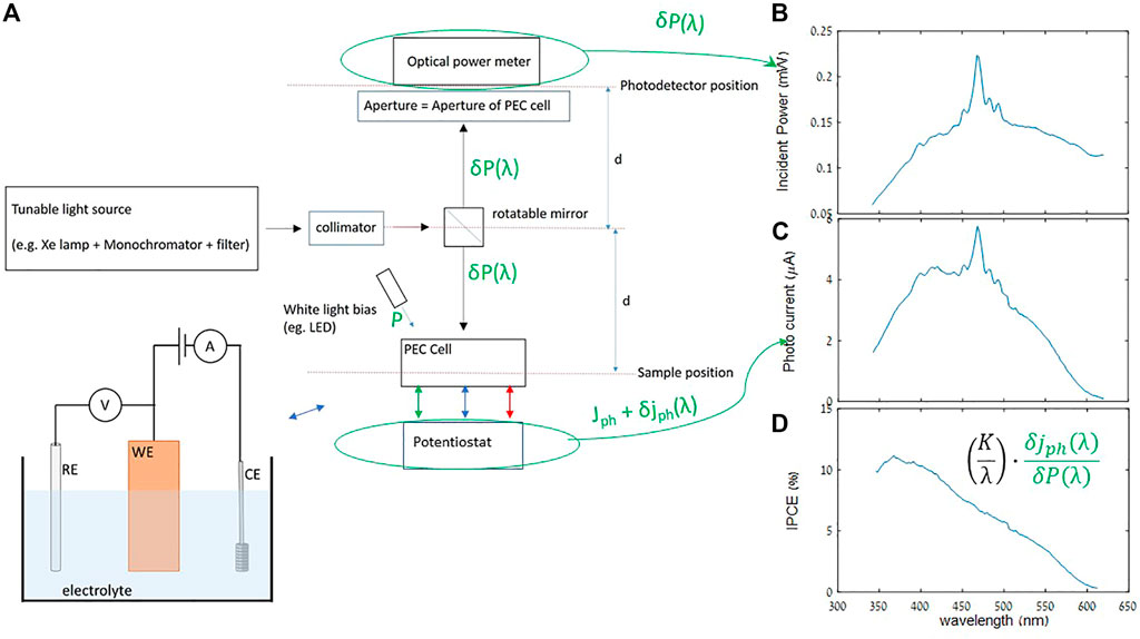
FIGURE 1. (A) Basic IPCE setup. The three-electrode mode voltammetry measurement setup of the current –potential (Jph-U) curve of the PEC cell (using a potentiostat) is illustrated schematically in the bottom left, with the sample serving as the working electrode (WE), a reference electrode (RE) and counter electrode (CE), all in contact with the electrolyte. Typical measurements of optical power (B) and photocurrent (C) spectra, resulting in IPCE spectrum (D), computed from the above with Eq. 1 Note that the bias light (of power P) from the LED leads to a bias photocurrent level (Jph) produced by the PEC cell, but the IPCE is determined from only the small signal values.
From the definition of IPCE as described by Eq. 1, it is common to relate the total expected photocurrent Jph to the IPCE spectrum (where both Jph and IPCE are measured at the same applied potential, U) by integrating the IPCE over the full wavelength range of the incident light spectrum S(λ). This is used to validate the consistency between the IPCE and photocurrent voltammetry measurements. Then, the spectrum of the light source can be replaced by the standard spectrum of the sunlight (typically the NREL AM1.5G standard) to calculate the expected photocurrent under 1-sun illumination conditions. Omitting unit conversion factors, for S(λ) units of photons per seconds per unit area per wavelength, we write for simplicity:
While Eq. 2 in many cases has been demonstrated to be exact within experimental error, and is indeed used as a standard check for consistency between the IPCE measurement and measured photocurrent, there are a number of subtleties to consider. In practice, because the monochromized (or sometimes also modulated) light signal P(λ) for the IPCE measurement could be relatively weak, Eq. 1 for IPCE should be considered to be a small-signal equation, measuring a small increase in current for a small increase in optical power. In contrast, Jph in Eq. 2 is a large signal quantity. Eq. 2 would be exact if IPCE were a constant (for a given applied potential U), independent of light intensity, but in some cases the small-signal IPCE spectrum could be dependent on light intensity [8]. This light-bias dependence is readily apparent simply by inspecting the dependence of Jph-U curves normalized by light bias. Figure 2 shows an example of Jph-U curves measured at different light intensities, and normalized by them, which cannot be explained by an intensity-independent IPCE spectrum at all applied potentials, even if one allows for series resistance to account for the photocurrent onset potential shifts. This issue regarding Eq. 2, has been highlighted previously (Christians et al., 2015; Shi et al., 2015), and up to 20% discrepancy can be commonly expected (Zimmermann et al., 2014). Before attempting to improve on Eq. 2, we should note that the mathematical complexity is increased because IPCE(λ) may not only be dependent on the light intensity at a given wavelength λ, but also on the total light intensity across all photon energies exceeding the bandgap. Physically, this determines the steady state photogenerated carriers, which can, in turn, affect the internal sample and surface conditions, and therefore have an influence on the IPCE.
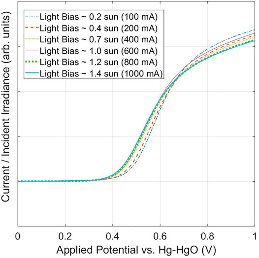
FIGURE 2. Photocurrent normalized by light intensity vs. applied potential, for various intensities of the LED white light source. The light intensity was determined by a fitted calibration curve of light intensity vs. LED current, the former measured with a spectroradiometer and integrated over wavelength for the total irradiance. The sample was a 26 nm thick epitaxial 1% Ti-doped hematite deposited on platinized sapphire.
Notwithstanding, we can proceed to a more exact variation of Eq. 2 if we consider a total-intensity-dependent IPCE (λ,U,β) where IPCE now also depends on total light intensity I via an intensity scaling factor β such that I = β ∫S(λ)·dλ. In this way, we can envision a “thought-experiment” in which we gradually increment the total intensity, while maintaining the spectral shape of the light source, by increasing β continually from 0 to 1, which in turn gradually increases the photocurrent accordingly until it reaches the final value. With this picture in mind, we write:
where the inner integral is over the full wavelength range determined on either side by the IPCE or S (λ) limits, whichever is more limiting. Re-writing to a form resembling the original Eq. 2:
where
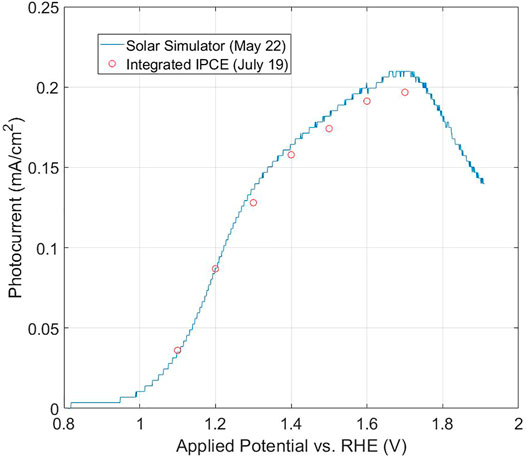
FIGURE 3. Integrations of Eq. 3b for IPCE of a hematite photoanode (measured in white LED light bias) vs. potential, compared to the Jph-U curve measured, on a different date, under solar simulator illumination. The sample was a 1% Sn-doped hematite layer, having 85 nm thickness, deposited on ITO, on an eagle glass substrate.
Especially for new and relatively untried types of photoanodes, we highly recommend to at least once characterize the typical light-bias dependence of the current–potential curves (as in Figure 2) to begin with (and if warranted, measurement of IPCE at a number of different light biases), in order to avoid potential misuse or mis-interpretation when attempting to validate the IPCE and/or Jph measurement with Eq. 2. So-motivated to measure IPCE under light bias, we caution that this introduces additional challenges in the measurement, but can be dealt with as shown in the next section. A final note regarding Eq. 2 or Eq. 3b is that ideally, S(λ) should be measured in the same sitting as the Jph–U measurement, to ensure that the actual S(λ) is used to integrate with the IPCE, not affected by possible changes in sample distance from the source, etc. This could be measured, for example, by a spectroradiometer put in place of the PEC cell. The IPCE measurement itself need not be done in the same sitting as the Jph–U or light source measurements (for example, see the dates between measurements in Figure 3), as long as the sample is stable over time and conditions such as applied potential and electrolyte are well replicated.
3 Mitigating Sources of Error and Noise
3.1 Description of Basic System and Measurement Procedure
In the following sub-sections we list or state a number of measurement trouble-spots and possible solutions, some of which are straightforward and self-explanatory (but nevertheless warrant brief attention as a reminder), but others requiring more elaboration which we provide with specific demonstrations and examples. As a starting point of reference, we begin with a description of our base system and procedure (before introducing modifications in subsequent sections), whose elements are likely typical for many IPCE systems, with only minor variations (a majorly different scheme, however, will be briefly touched upon in Section 3.4). Our measuring system, depicted schematically in Figure 1A, is based around the Oriel QV-PV-SI “Quantum Efficiency Measurement Kit,” by Newport. The work area at the IPCE station is enclosed in a black curtain and ambient light (as can be monitored on the power meter) is kept to a minimum; ambient light from instrumentation panels and computer screens is low enough for the power meter reading to be at its noise floor and likewise does not produce significant photocurrent (as a comparison, the few 100 μW of monochromatic light in Figure 1B, which in the dark looks quite bright on the sample, produces a few μA of photocurrent, but the ambient light is relatively dim, perhaps several hundred times less). The probe light is generated from a broadband Xe lamp source (up to 1 kW input power) monochromatized by a Cornerstone 260 monochromator. The output light is collimated and focused with the appropriate optics. Collimation of the beam plays the important role of decreasing the sensitivity of the beam cross-sectional profile to small changes that could inadvertently occur in distance between mirror and sample or power meter, in spite of efforts made to make these distances consistent. The aluminum mirror shown at the center of the system illustration presented in Figure 1 could be manually rotated so as to direct the light to either the power meter or PEC cell (i.e., the sample), with grooves on the mirror stage restricting the possible angles to discrete values to ensure repeatability and proper placement of the angle. On the PEC cell side, the photoanode is placed in a “cappuccino” cell (Cesar 2007), and connected in 3-electrode mode to a potentiostat (Zahner Zennium in our system). Our typical sample has a transparent current collector layer (typically a doped tin oxide layer, fluorine-doped FTO or niobium-doped NTO, or a tin-doped indium oxide layer ITO), with the photoanode layer (i.e. hematite, and possible underlayers and overlayers) deposited over part of it. Typical hematite samples produced in our group were deposited by pulsed laser deposition either on a tin-doped indium oxide (ITO) (Piekner et al., 2018), niobium doped titanium oxide (NTO) conductive layer (Grave et al., 2016b), or platinum conductive layer (Grave et al., 2016a) on sapphire, or on eagle glass substrates for polycrystalline films. The working electrode lead is connected with an alligator clip to the exposed transparent correct collector layer, with the hematite layer partially in contact with the electrolyte (1M NaOH aqueous solution, pH 13.6), through the aperture (3.7 mm when measuring samples with sapphire substrates, or 6 mm diameter for larger samples having eagle glass substrates) of the cappuccino cell. An Hg/HgO/1M NaOH reference electrode (ALS model RE-61AP, appropriate for use in alkaline solutions), and platinum counter electrode (ALS model 012961), are immersed in the electrolyte and likewise connected to the potentiostat with alligator clips. This is shown schematically in the bottom left of Figure 1A.
Prior to making electrical connections, the optics is inspected to ensure that the (monochromatic) beam profile on the aperture to the power meter is identical to the beam profile incident to the aperture on the cappuccino cell. After connecting the alligator clips, the electrical connection is checked by, in our case, making an impedance measurement (typically at 10 kHz frequency, to bypass usual capacitive effects from electrochemical interfaces) using the a.c. capabilities of the potentiostat which is coupled to a frequency response analyzer (FRA) in our Zahner Zennium potentiostat. In the case of our typical samples, we consider 200 Ω and below to indicate a reasonably good connection; if our typical photocurrent is maximum 200 μA, then this amounts to an error of ∼40 mV at most, which could represent a significant offset (i.e. see Figure 2), but on the other hand could be accounted for and does not qualitatively impact the measurement, as compared to a “bad connection” which is typically 1 kΩ and higher, and is usually a sign of an ill-placed or corroded alligator clip. The next step after the probe beam optics and electrical connections are set, is to arrange the white-light bias so as to produce an expected amount of photocurrent for a given applied potential. In our setup, a broadband, high power LED (Mightex Systems, 6500 K “glacial white” spectrum, 300 mW maximum radiant flux, which could output an order of ∼1 sun equivalent intensity on the sample) is positioned to obliquely shine on the sample, as depicted in Figure 1A, so as not to block the incident monochromatic beam. The usual procedure is to modify the incident angle of the light bias to center its circular profile on the sample, monitoring the photocurrent in real time to maximize it. The light level can be subsequently adjusted by changing the LED current via software.
After the above preliminary checks and setups, a current-potential scan under light bias is performed. These may be repeated until the sample stabilizes (i.e. the current-potential curves are repeatable), and further adjustments to the light bias current may be made to achieve the desired condition for the IPCE measurement (i.e., typically to replicate a Jph-U scan made elsewhere, or set β to a specific value). For our hematite samples, we found that 20 mV/s was an adequately slow sweep-rate, but this may vary depending on the sample. We note that the photocurrent is obtained by subtracting the dark current vs. applied potential scan from the scan made under light. Once the applied potential and white light bias are set for the IPCE measurement, a certain time may be allotted for stabilization, which may also be monitored in real time by continuous measurement of the photocurrent.
Having set the operating condition, including fixing the applied potential and light bias, the basic IPCE procedure is relatively simple. First the mirror is rotated to direct the monochromatic beam to the power meter, and a scan of optical power vs. wavelength is performed. Then, the mirror is rotated for sample illumination and the same wavelength scan repeated, but this time measuring current on the potentiostat. The baseline current, measured with the same light-bias, but without any monochromatic beam, is subtracted to produce δjph(λ), and Eq. 1 applied for the IPCE spectrum. Usually, another P(λ) scan is done afterwards to check stability of the monochromator, discussed in Section 3.4 below. We found this method to be adequate in the case of zero light bias (β = 0), whereby the LED would only be used to check the Jph-U curve for the purpose of setting the applied potential to a certain operating point, but then turned off for the IPCE scans. However, in the case of light biases approaching 1-sun intensity (β = 1), it fails spectacularly. In the sub-sections below we discuss some of the finer points of different aspects of the measurement.
3.2 Optical Power Measurement
The basic optical power measurement is fairly straightforward. Here we just briefly review a few points. As described above, one should be careful to keep the optical power (i.e. beam-profile) the same on the power meter as on the sample, by use of appropriate apertures, and symmetric geometry etc., which should be confirmed by appropriate distance and height measurements and visual inspection, to verify proper centering of the incident beam profile on the sample and photodetector. The power meter should be calibrated according to wavelength, ideally NIST traceable, and informed of the correct wavelength at each point in the scan. As the power measurement time could be rather quick (several readings per second), fluctuations can be reduced by repeated averaging (or longer integration times) of measurement without much additional cost in scan time. To be optimal, this could be adjusted to be comparable to the overhead time of each wavelength point, or some fraction thereof. If the ambient environment is dark, there will usually be negligible background for most of the scan, but as can be seen from the Xe lamp (plus monochromator grating/filter) spectrum in Figure 1B, the power can fall off significantly at the extrema of the wavelength range. If the scan must necessarily include such low-power ranges, the electronic noise-floor of the power meter may dominate the reading. In this case, a background (in the dark) scan of the power meter should be done first and subtracted wavelength-per-wavelength. We found, however, that a few wavelength points plus linear interpolation, lasting only a few seconds total, are adequate for the background scan. Lastly in this section, although perhaps not solely a power issue, we emphasize the importance of correct use of optical filters (which cut off low wavelengths) appropriate to the wavelength range (or vice-versa) during the monochromatic scan, in order to block higher order diffraction passed by the monochromator gratings. Although the higher harmonics may have a relatively small effect on the total power, they can have a significant impact on the photocurrent–for example, if at a photon energy below the sample’s optical bandgap, there should be practically no photocurrent, but a second harmonic could have energy above the bandgap, and produce significant (and misleading) photocurrent. Additionally, the typically wide-bandgap transparent conducting layers (i.e., FTO, ITO or NTO) may also activate from short-wavelength second harmonics.
3.3 Current Measurement and Current Drift
Current drift during measurement is the main killer when it comes to measuring in light bias, and is the likely reason many published works to date have avoided presenting IPCE measurements in light bias. Very simply, the optical power of the monochromatic probe beam is typically much weaker than the ∼1 sun white-light bias intensity, and thus the resultant photocurrent signal is correspondingly weaker. A factor of 100 is not unusual, depending on the wavelength and lamp condition. Therefore, merely a few percent drift of the current under bias over the time of a typical wavelength scan (which could be ∼½ h or more, depending on the wavelength stepsize, etc., and could easily be caused by gas bubbles or other effects) could produce a significant error, in either direction, to the measured δjph after subtracting the light bias contribution, and thus to the IPCE. This is illustrated in Figure 4A, which shows reasonable looking IPCE values for zero light bias (0 mA LED current), but an artifact decrease, even to negative IPCE values, at low wavelengths when a ∼ 1-sun bias (1,000 mA LED current) is applied. The inset shows the measured total current under light bias, which looks relatively stable on an absolute scale, but the slight decrease near the end of the scan (from high to low wavelength) causes a precipitous decrease of the calculated IPCE, which is clearly an artifact.
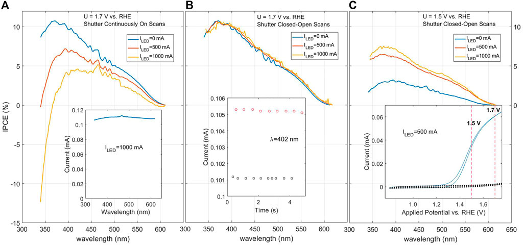
FIGURE 4. IPCE scans on a 30 nm Ti-doped hematite film deposited on a platinized sapphire substrate, for different light bias intensities (1000 mA LED current is comparable to 1 sun). (A) Measured by the base system and method, before the shutter on-off method was implemented. In this case, the current is measured as the monochromator is incremented from high to low wavelengths. The inset shows the total measured current (including from the light bias) of such a scan under strong light bias. The applied potential was set to 1.7 V RHE, near the plateau region as indicated in the inset of (C). (B) Using the shutter closed-open scheme. The inset shows the current vs. time measurements for one of the wavelength points, with shutter open in red (upper), shutter closed in black (lower). (C) Using the shutter open-closed scheme, but for the applied potential lowered to 1.5 V, which is below the plateau region of the Jph-U curve, shown in the inset; dark current is shown as the black dashed line.
One solution to take into account this current drift is to subtract the baseline current (the current under the light bias used, but without the monochromatic small signal light), such that the “mono-light on” and “mono-light off” current measurements are done at almost the same time (only a few seconds apart) at each wavelength. We initially implemented this by simply using the slits in the monochromator as an effective shutter: opening and closing them at each wavelength, and measuring current as a function of time for each of the shutter-open and shutter-closed states, as shown in the inset of Figure 4B. The improvement of using the shutter on-off scheme is immediately apparent in Figure 4B, where the measured IPCE spectrum does not change with light bias, even up to ∼1 sun at LED current of 1,000 mA. Figure 4C shows that when the applied potential is lowered to be below the plateau region of the Jph-U curve, indicated in the inset, there appears to be a systematic drop in the IPCE for this sample as the light bias is lowered. Given the consistency of the measurement in the plateau region shown in Figure 4B, we can plausibly make the distinction that this is truly a sample condition effect of non-linear sensitivity to light intensity in the near-onset region, and not a measuring artifact like in Figure 4A.
To examine more closely the dynamics that could occur in the PEC cell during the IPCE measurement, the current vs. time response upon opening or closing the monochromator shutter (λ = 582 nm), for another hematite sample, is shown in Figures 5A,B for zero light bias and ∼1 sun white light bias, respectively. We note that jph(λ) in Figure 5B is less than 1% of the current due to the light bias. For the case without light bias, Figure 5A, we see a relatively slow decay in the current response to opening and closing the monochromator shutter, lasting several seconds before the current reaches steady state. The photocurrent jph(λ) is taken as the difference between the (approximately) steady state values. The dynamics with light bias, Figure 5B is somewhat faster, but still with a settling time of the order of ∼1 s. This variation in settling time could be understood in terms of charging and loss mechanisms at the surface, which has also been demonstrated by modulated techniques and related distribution of relaxation time (DRT) analysis (Peter 2013; Klotz et al., 2016; Klotz et al., 2018). This sometimes-slow dynamics is a reason for caution related to using the popular phase-locked loop (PLL) technique with a lock-in amplifier for measuring the small-signal IPCE, which indeed can overcome the drift (and other) problems, but if the modulating frequency is higher than 1 Hz (which is typical for PLL), may miss such slow loss mechanisms, erroneously measuring the higher δjph(λ) seen at the beginning of the transient response. This is more likely to occur at lower applied potentials where surface recombination dominates. Frequency dependence issues of IPCE have also been studied for perovskite materials (Ravishankar et al., 2018) and dye-sensitized solar cells (Xue et al., 2012).
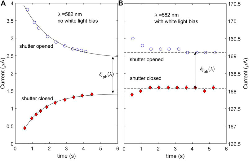
FIGURE 5. Effect of light bias on small-signal photocurrent response to a step in the light intensity. The sample was a 1 μm thick, Ti-doped hematite layer over an FTO conductive layer, measured with monochromatic light incident on the back of the sample. The applied potential was set to 1.6 V RHE, well above the photocurrent onset (at ∼1.2 V RHE, not shown), but near the onset of dark current (A) Without light bias (B) with ∼1 sun white light bias, incident on the front of the sample. Note that the photocurrent scale spans the same 4 μA as in (A), but offset by the current contribution from the LED bias (∼ 166.5 μA).
3.4 Light Source Drift and Noise
Another source of error in the IPCE measurement, usually less dramatic than photocurrent drift, but still potentially significant, is drift and/or noise of the light source for the monochromatic beam. In many IPCE setups including our own, the light source is a Xe lamp. However, it is a fitting juncture to make mention of an alternative technology which was developed at the National Renewable Energy Laboratory (Young et al., 2008). In this concept, light from an array of several LED’s, each emitting a different wavelength spanning the spectral range, is simultaneously focused on the sample. The LED’s are each modulated with a different frequency, so data processing can isolate the contributions to the generated photocurrent from each wavelength via the Fourier transform of the photocurrent, which in Fourier space will have a peak for each modulation frequency. In this way, the whole spectral range is measured at once, drastically reducing the time required to measure each IPCE spectrum, and can be as short as a second (for high frequencies). This method is currently employed in a number of commercial systems. Many of the drift-related problems can be totally avoided, however the modulation frequencies (and thus speed) would still subject to the system frequency limitation described in the previous section. Anticipated disadvantage of an LED array as opposed to Xenon source plus monochromator, would be less access to the UV portion of the spectrum, and also somewhat less wavelength resolution (or sharpness) based on the inherent LED bandwidth limitations as compared to the monochromator, and discrete separation of the LEDs. Evaluating these quantitatively is beyond the scope of this paper. The approach certainly deserves serious consideration, depending on the system being measured, but we here we proceed to deal with the problems and procedures for using the conventional Xe lamp and monochromator.
A common practice is to allow an hour or half an hour time after turning on for the lamp to stabilize before commencing the IPCE scans. However, as shown in a sequence of repeated lamp scans over 6 hours in Figure 6, fluctuations in lamp power from one scan to another, can occur well past this initial warmup time. While several scans in a row show intensity that is relatively stable (∼2% or better), occasionally larger shifts of lamp power also occur, of the order of ∼10%. While this allows the viability of checking the lamp stability immediately before and after each δjph(λ) measurement, should one be unlucky enough to have measured between the big jumps of the lamp, it would mean repeating the measurement/waiting until the lamp is stable again, amounting to a considerable cost in time.
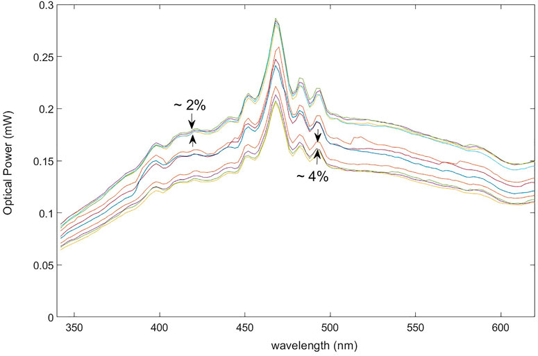
FIGURE 6. Series of monochromator scans of a Xe lamp over a period of 6 h. Some typical shifts, during the periods of relative stability between the larger jumps of intensity, are indicated as a percent error.
The above problem would be largely circumvented if, similar to the shutter on-off measurements in the previous section, the optical power were also measured at every wavelength point. There are a number of different approaches to achieve this, each having advantages and drawbacks. One approach (Palma et al., 2015) used the optical architecture of a Lambda 35 spectrophotometer, which featured a beam splitter to divide the incident beam to simultaneously measure the incident power. A slight complication of the beam splitter approach is that, from surveying vendor’s websites, even beam splitters designed for broadband applications seldom exhibit completely uniform or consistent splitting ratios over a wide wavelength range, so a careful calibration, requiring two calibrated (ideally identical) photodetectors, would be needed to characterize the splitting ratio as a function of wavelength. In principle, however, this calibration need be done only once.
As an alternative method, we automated the rotation of the mirror in our setup which was previously done by hand between scans, allowing the mirror to switch angles to direct the light between the power meter and the PEC cell for every wavelength. This has the advantage of measuring (in principle) the exact same light beam incident on the PEC cell, aside from possible errors in motor motion, or power fluctuations that could occur on a few-second scale, which in practice was usually not large (with exceptions, discussed below). The main challenge with this method is precise and consistent control of the motor angle. Our rotary stage was a HR-3 model from Newmark Systems, with an NSC-A1 stepper motor controller. Inclusion of an encoder which independently measured the angle was crucial for ensuring the correct angles, and we incorporated stabilization routines and checks in our software control. In practice, a 0.1° repeatability in angle was achieved with relatively fast motions (∼1 s position switching time), resulting in negligible variation in detected power or current. Each time upon startup of the IPCE system, we performed a brief (few minutes) but effective angle zeroing procedure whereby a small aperture is temporarily placed in front of the monochromator output, and the mirror angle zeroed by back-reflecting the beam back unto the aperture. Even relatively tiny IPCE’s could be resolved with relatively little fluctuation. This sensitivity is also largely thanks to the resolution of the Zennium potentiostat (by Zahner), which can accurately resolve down to the level of nA currents. The ability to measure low IPCE’s could be useful, for example, to characterize device behavior outside the normal operational range, such as energies near or below the band-edge, or a low applied potentials. Figure 7, adopted from (Grave et al., 2021), shows IPCE spectra (Figure 7B) measured at different applied potentials along the Jph-U curve (Figure 7A). As the cyan spectrum around 500 nm and scaling factors in the legend of Figure 7B show, IPCE spectra with values down to ∼0.001% can be at least roughly measured. An added benefit of the motorized mirror method is that, in addition to measuring the optical power at each wavelength, the light-off current may also be measured by directing the beam away from the PEC cell, thus also filling or replacing the “shutter on/shutter off” role described in the previous section.
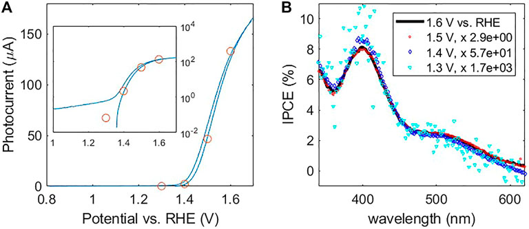
FIGURE 7. IPCE measurements at different applied potentials along the Jph-U curve of a 1% Sn-doped 7 nm hematite film deposited on ITO-coated glass substrate (A) Jph-U curve, with circles indicating the applied potentials at which IPCE measurements were made and their corresponding integrations with the LED spectrum according to Eq. 3b. The inset plots the same, but with the photocurrent axis on a log scale. (B) IPCE spectra measured at the different applied potentials, in white light bias shown in the legend. The measured spectra were scaled up by multiplying by the factors indicated in the legend. Adapted from Supplementary Figure S4 of (Grave et al., 2021).
One situational disadvantage of the motorized mirror stage scheme, which might be in some respects better handled with the beam splitting approach, is if lamp fluctuations occurred over the same timescale as the delay between mirror rotations (typically a number of seconds). Ideally the Xe lamps are designed to not normally exhibit such fast intensity fluctuations, but we nevertheless found this to be the case from time to time. We noticed that in these situations, the spectra markedly improved and the noise disappeared in the evening hours, when other electronic devices in the building or vicinity were likely not as active. We consequently attributed the short-term fluctuations to electromagnetic interference (EMI) or other noise coming from the operation of other devices in the vicinity of the experiment, perhaps from adjacent rooms or floors, or outside. bXe arc lamps and similar plasma-based devices can be particularly sensitive to electrical noise including from EMI, in part due to thermal stresses and turbulent convection flows within the lamp, and there have been studies of these issues (Green et al., 1968; Rolt et al., 2016). Therefore, EMI could be a possible issue to consider, which could be mitigated by additional shielding or regulation, or more simply by measuring in a time and/or place where less EMI or other external noise is likely to occur. Sensitivity to electronic noise may also be a function of the age of the lamp, which should be periodically replaced.
3.5 On Software: Handshaking With Machines but Holding Hands With Humans
We conclude this section by briefly digressing from the science/instrumentation side to discuss a nonetheless important part of effective IPCE measurements: the software interface. The core goal of IPCE software is to synchronize the actions of the rather diverse collection of instrumentation participating in an IPCE measurement–for the system outlined here this includes monochromator, potentiostat, optical power meter, and motorized mirror stage–integrating their control into a single program capable of properly orchestrating the measurement according to the experimenter’s specifications. This could be implemented by such programs as Labview, as was done in this work. But to truly be effective, the “user friendliness” aspect should not be neglected. This includes an intuitive and easy-to-learn interface, active anticipation and prevention of common human error (such as checking if the typed data-save directory or filename exists before the scan starts, and prompting the user if there is a suspected problem with either files or devices to take corrective action), accommodation of situations such as the need to pause the scan mid-way to remove bubbles (especially important for measurements under light bias) and bubble-related spike-removal options, communicating and updating status (such as the applied potential) to the user so they can easily spot problems in real time, and convenient (but controlled) access to peripheral functions, such as opening popups that allow manual control of the monochromator or rotary stage, etc. In the case of Labview, a “stop” button is default to all programs, yet can present a hazard in that it allows users to arbitrarily and easily interrupt the program at any time, typically for reasons that could have been prevented or otherwise handled, and with potentially costly end-results of very possibly requiring resets of machines (and in the case of our rotary motor, even re-zeroing of the position). This button can be replaced with a more controlled abort and shutdown mechanism. In short, what we describe amounts to pro-active prevention of problems by tight control of the measuring process flow, but at the same allowing user flexibility in a “safe” manner. These features were implemented in our software, largely motivated by the experience (and frustrations) of ourselves and other colleagues and students measuring IPCE at various stages of development of the system. Figure 8 shows some sample screenshots of our Labview interface including such features. Visual cues and audio cues (such as end-of-scan announcement) were also incorporated for enhanced awareness (and, a little bit, fun variety) during the measurements.
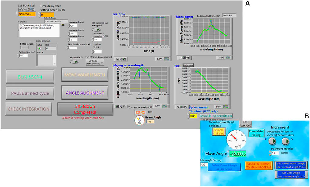
FIGURE 8. Screenshots of the software interface used for the IPCE system: (A) Interface with scan settings and large buttons for the main, often-used functions, such as beginning the scan and pausing. Plots of the on-off transient current, photocurrent (before automatic spike removal, which can be user-specified), optical power, and resultant IPCE spectra update point-by-point during the scan. The large buttons also dynamically display messages such as status messages (like “setting potential,” etc.), and/or instructional messages (like “press to resume scan” after pausing), or open pop-ups, such as (B) a pop-up window for manual control and calibration of the mirror angle.
4 Incident Photon to Current Efficiency Measurements of BiVO4 Ultrathin Film Photoanodes Under White LED Bias
Recently, some of us undertook to measure the IPCE of BiVO4 photoanodes under light bias. Light intensity dependence and photodegradation of BiVO4 photoanodes under PEC operation is a well-known issue with these types of photoanodes, and has been studied by various groups of authors for more than a decade (and counting), including but not limited to references (Sayama et al., 2006; Abdi and van de Krol 2012; Toma et al., 2016; Zhang et al., 2019; Kou et al., 2020; Zhang et al., 2020). Nevertheless, the photocurrent under our white LED bias appeared to be relatively stable, decreasing ∼3% during a typical scan. From this (deceptively) stable photocurrent, one might reasonably assume as a corollary of Eq. 2 or Eq. 3b that the IPCE spectrum should likewise be stable. As later became apparent, this was not to be the case. Nevertheless, it makes for an interesting case study of an unexpected situation that can occur when measuring IPCE on unknown samples, and the IPCE data obtained may offer some new lines of investigation for further studies of the IPCE decrease, although the latter is beyond the scope of this manuscript, and from this point of view we present this final section.
The samples were 30 and 10 nm thick BiVO4 films deposited by pulsed laser deposition (Kölbach et al., 2020) for which zero-light bias IPCE measurements of the 10 nm film were recently published (Grave et al., 2021). Our original intention for the latter work was to measure under light-bias, as was done for hematite photoanodes. We describe the procedure, which was approximately identical for both samples. The Jph-U curves were measured with the LED current set to 1,000 mA, shown in Figure 9A as solid lines. This LED intensity roughly corresponded to an overall photon flux of the same order of magnitude as 1 sun intensity. The first IPCE measurements were done under the same light bias, with the applied potential set to the plateau region (as shown by the crosses in Figure 9A, which also correspond to Eq. 3b integrations). These initial IPCE spectra in strong light bias are shown as yellow lines in Figures 9B,C for the 30 and 10 nm samples, respectively. Then, the PEC cell was rotated 180° so as to illuminate the back of the sample with the monochromator light, while also moving the LED around so as to continue to illuminate with the light bias on the front, and IPCE measurements were done with back illumination (not shown). Additional UV measurements were performed (not shown), and the sample and LED once more re-positioned to repeat the front (monochromator) illumination scans. By the time the 2nd front-illumination IPCE scan was started, the sample had been under the LED illumination for approximately 2 h (with brief interruptions rotating the sample, etc). The 2nd IPCE scans with front illumination are shown as purple lines in Figures 9B,C. The 10 nm film especially showed dramatic decrease of the hump at low wavelengths between the two front illumination measurements. For the 30 nm film there is a significant change between 1st and 2nd measurements, but not as dramatic. This is likely because even before the first measurement, the sample was already under illumination for some time while trouble-shooting a technical issue with the alligator clip, so was already in a decreased-IPCE state (possibly light-soaked; see for example, Wing et al., 2015) by the time the first measurement commenced. After observing these dramatic changes, the electrodes and electrolyte were removed, and sample allowed until the next day (∼14 h) to recover to their original surface state.
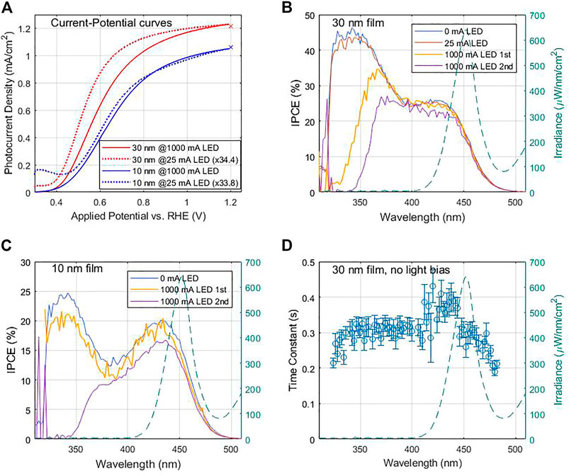
FIGURE 9. Measurements of 30 and 10 nm thick BiVO4 samples measured in a neutral buffer solution with a hole scavenger; details in (Grave et al., 2021). (A) Jph-U curves for 30 nm (blue) and 10 nm (red) thicknesses, under white-light LED bias of ∼1 sun (solid) and low-intensity (dotted). The x’s at 1.2 V indicate the applied potential where the IPCE was measured as well as the resultant integrations of Eq. 3b (B) IPCE spectra for the 30 nm film at various light intensities. The measurement sequence is described in the text. The LED spectrum is overlaid on the right y-axis (teal color). Zero-bias IPCE data obtained from (Grave et al., 2021). (C) IPCE spectra for the 10 nm film at various light intensities. The measurement sequence is described in the text. The LED spectrum is overlaid on the right y-axis (teal color). Zero-bias IPCE data obtained from (Grave et al., 2021). (D) Fitted time constant of the step-response vs. wavelength, measured during the IPCE measurement without light bias, for the 30 nm film. The LED spectrum is overlaid on the right y-axis (teal color).
When the measurements commenced the following day, it was without exposing the sample to a strong light bias, in order to avoid the time-dependent effects observed above. Even the Jph-U curves, usually done before each IPCE measurement to verify a consistent operating potential relative to them, were done with the LED current set to only 25 mA. These low-intensity curves are shown as dotted lines in Figure 9A, scaled as indicated in the legends by a factor of ∼34 which was similar for both samples so the shapes and onset potentials may be compared. We attribute the larger potential shift for the 30 nm sample to a larger series resistance, but otherwise the shape of the Jph-U curves were fairly consistent with the previous day’s high-intensity scans. The IPCE curves for 25 and 0 mA LED biases, respectively, are plotted as red and blue curves in Figures 9B and a large low-wavelength hump appears, qualitatively similar to that of the 10 nm sample, approximately the same for both low intensities. For the 10 nm film in Figure 9C, the zero light-bias IPCE measurement (the 25 mA was skipped) showed very similar IPCE to the 1st light bias measurement the previous day. Repeated zero light-bias IPCE measurements for both films were found to be consistent, so the sample was stable in zero light-bias conditions.
These results together indicate that not only is there a light-bias effect, but also a slow decrease of parts of the IPCE spectrum in sustained light bias. But what appears to be the most unexpected and, in some sense, perplexing/counter-intuitive behavior, is that the spectral portion of the IPCE which is encompassed by the spectrum of the LED is relatively stable, while the unstable part is outside of the LED spectral coverage. The latter is plotted as dashed lines in Figures 9B–D, showing that the LED itself causes a dramatic decrease of the higher-energy (lower wavelength) part of the IPCE, which is well outside its own spectral range. A physical model that could explain this behavior is outside the scope of this manuscript. One additional indicator could perhaps be in the time constants of the photocurrent step-response (i.e., like plotted in Figure 5A for example). The step responses, recorded for each wavelength as part of the IPCE measurements described in Section 3.3, were fitted to an exponential decay for each wavelength and plotted in Figure 9D. The time resolution of our measurements was relatively poor, only 0.5 s intervals, and the 10 nm sample’s response became stable too quickly for us to fit, but the 30 nm sample was slower (consistent with a larger series resistance, as indicated by the onset potential shift in Figure 9A), and the decay could be somewhat resolved and fitted at most wavelengths (far outliers were excluded from the plot). As Figure 9D shows, while the time constant is steady between 350 and 400 nm, there appears to be a distinct increase above ∼410 nm and then falls off again beyond ∼450 nm. Comparing against the IPCE curves in Figure 9B above, there might be some correlation between the time constants, and the stable and unstable regions of the IPCE spectrum. This could be an avenue to investigate in further studies using smaller time steps and more systematic measurements, which should also include dependence on applied potential as well. We note that similarly prepared samples, but with 90 nm thick BiVO4 layers, were used in a recent photocorrosion study (Zhang et al., 2020). In our case, the relative stability of the IPCE within the LED spectrum gave rise to the observed stability of the photocurrent, which only changed a few percent during the scans. The crosses in Figure 9A, at 1.2 V, are the integration of the (10 and 30 nm) IPCE spectra with the LED spectrum according to Eq. 3b and which works well because the IPCE in the LED’s spectral region is mostly independent of light-bias intensity of the LED, and is stable over time. Under a spectrum more resembling the solar spectrum, which has lower-wavelength spectral weight, the photocurrent would be expected to decrease with time more dramatically, as has indeed been observed in the literature. Subsequent to this preliminary measurement, we observed similar time dependence of the IPCE spectrum for thicker BiVO4 samples under white light bias, which will be presented elsewhere.
In summary, we reviewed the basics and expanded on some of the finer technical points of IPCE measurements in PEC systems, using primarily hematite as a model system for examples. Emphasis was placed on demonstrating the importance (depending on the linearity of the photo-response) and difficulties of measuring the sample under white light bias, which along with applied potential sets the operating point to a large-signal photocurrent. The wavelength-resolved light source used for the small-signal probe was based on a Xe lamp with scanning monochromator. Because of the considerable amount of wavelength points for the scan, combined with upper limit on the photo-electrochemical frequency response (or lower limit on measurement time required), the total measurement time for an IPCE scan can take several minutes or even half an hour. During this time, two distinct problems can occur, drift of the large-signal photocurrent under white light bias, due to small changes in the sample or its environment, or change in the Xe lamp’s output. These can be remedied by measuring the optical power, and the small-signal photocurrent (both with and without monochromatic light) at each wavelength point. We accomplished this by using a rotary mirror, but it is by no means the only possible solution, and the advantages and potential drawbacks of various alternatives, including the lock-in technique, beam-splitter, and the “flash” IPCE technique, were discussed. The IPCE spectra measured with our final system was demonstrated to be consistent (when integrated over the incident light spectra) with large signal photocurrent (Figures 3, 7A), and spectral shape repeatable under light bias for different LED intensities (in the linear regime, Figure 4B), and applied potentials (and able to resolve miniscule signals, Figure 7B). In the case study of BiVO4 photoanodes, the measuring system so-modified to minimize drift effects allowed us to attribute the observed time-dependence under light bias to actual behavior of the photo-electrochemical system under test, rather than to the measuring system.
Data Availability Statement
The original contributions presented in the study are included in the article, further inquiries can be directed to the corresponding authors.
Author Contributions
DE wrote the first draft of the manuscript and did the system development work described herein, and measured or closely guided assistants measuring the presented data. DG and YP. grew the various hematite samples measured, helped with some of the IPCE measurements, and helped with the subsequent drafts of the manuscript. PS grew the BiVO4 samples and helped with the subsequent drafts of the manuscript. AR is the principle investigator who initiated this work and worked carefully especially on the initial edits of this manuscript.
Funding
The research leading to these results has received funding from the PAT Center of Research Excellence supported by the Israel Science Foundation (grant no: 1867/17). The IPCE measurements were carried out at the Technion’s Photovoltaics Laboratory (HTRL), supported by the Russell Berrie Nanotechnology Institute (RBNI), the Nancy and Stephen Grand Technion Energy Program (GTEP) and the Adelis Foundation. Part of this research was carried out within the Helmholtz International Research School “Hybrid Integrated Systems for Conversion of Solar Energy” (HI-SCORE), an initiative co-funded by the Initiative and Networking Fund of the Helmholtz Association. Part of the work was funded by the Volkswagen Foundation. DG and DE acknowledge support from the Center for Absorption in Science at the Ministry of Aliyah and Immigrant Absorption in Israel. YP acknowledges support by the Levi Eshkol scholarship from the Ministry of Science and Technology of Israel. AR acknowledges the support of the L. Shirley Tark Chair in Science.
Conflict of Interest
Author PS is employed by Helmholtz-Zentrum Berlin für Materialien und Energie GmbH. All authors declare no other competing interests.
Publisher’s Note
All claims expressed in this article are solely those of the authors and do not necessarily represent those of their affiliated organizations, or those of the publisher, the editors and the reviewers. Any product that may be evaluated in this article, or claim that may be made by its manufacturer, is not guaranteed or endorsed by the publisher.
Acknowledgments
DE would like to thank Yossi Levi who acquainted him with IPCE measurements and initial system, which was in large part set up by Gideon Segev, and introduced him to some of the issues discussed herein, and is grateful to Dr. Guy Ankonina for his constant technical support and willing assistance whenever needed or asked for in the Photovoltaics Laboratory at the Technion. Many thanks to Sofi Yanru, Ortal Tiurin, Rotem Yaniv and Alon Inbar for assisting with the measurements throughout the various stages of this work.
References
Abdi, F. F., and van de Krol, R. (2012). Nature and Light Dependence of Bulk Recombination in Co-pi-catalyzed BiVO4 Photoanodes. J. Phys. Chem. C 116, 9398–9404. doi:10.1021/jp3007552
ASTM Standard E1021-15 (2019). Standard Test Method for Spectral Responsivity Measurements of Photovoltaic Devices. West Conshohocken, PA): ASTM International.
Bahro, D., Koppitz, M., and Colsmann, A. (2016). Tandem Organic Solar Cells Revisited. Nat. Photon 10, 354–355. doi:10.1038/nphoton.2016.96
Cesar, I. (2007). Solar Photoelectrolysis of Water with Translucent Nanostructured Hematite Photoanodes. Lausanne: EPFL.
Chen, Z., Deutsch, T. G., Dinh, H. N., Domen, K., Emery, K., Forman, A. J., et al. (2013). “Incident Photon-To-Current Efficiency and Photocurrent Spectroscopy,” in Photoelectrochemical Water Splitting Standards, Experimental Methods, and Protocols. N. Gaillard, R. Garland, C. Heske, T. F. Jaramillo, A. Kleiman-Shwarsctein, E. Milleret al. (New York: Springer), 87–97. doi:10.1007/978-1-4614-8298-7_7
Christians, J. A., Manser, J. S., and Kamat, P. V. (2015). Best Practices in Perovskite Solar Cell Efficiency Measurements. Avoiding the Error of Making Bad Cells Look Good. J. Phys. Chem. Lett. 6, 852–857. doi:10.1021/acs.jpclett.5b00289
Grave, D. A., Dotan, H., Levy, Y., Piekner, Y., Scherrer, B., Malviya, K. D., et al. (2016a). Heteroepitaxial Hematite Photoanodes as a Model System for Solar Water Splitting. J. Mater. Chem. A. 4, 3052–3060. doi:10.1039/c5ta07094e
Grave, D. A., Ellis, D. S., Piekner, Y., Kölbach, M., Dotan, H., Kay, A., et al. (2021). Extraction of mobile Charge Carrier Photogeneration Yield Spectrum of Ultrathin-Film Metal Oxide Photoanodes for Solar Water Splitting. Nat. Mater. 20, 833–840. doi:10.1038/s41563-021-00955-y
Grave, D. A., Klotz, D., Kay, A., Dotan, H., Gupta, B., Visoly-Fisher, I., et al. (2016b). Effect of Orientation on Bulk and Surface Properties of Sn-Doped Hematite (α-Fe2O3) Heteroepitaxial Thin Film Photoanodes. J. Phys. Chem. C 120, 28961–28970. doi:10.1021/acs.jpcc.6b10033
Green, M., Breeze, R. H., and Ke, B. (1968). Simple Power Supply System for Stable Xenon Arc Lamp Operation. Rev. Scientific Instr. 39, 411–412. doi:10.1063/1.1683394
Klotz, D., Ellis, D. S., Dotan, H., and Rothschild, A. (2016). Empirical in Operando Analysis of the Charge Carrier Dynamics in Hematite Photoanodes by PEIS, IMPS and IMVS. Phys. Chem. Chem. Phys. 18, 23438–23457. doi:10.1039/C6CP04683E
Klotz, D., Grave, D. A., Dotan, H., and Rothschild, A. (2018). Empirical Analysis of the Photoelectrochemical Impedance Response of Hematite Photoanodes for Water Photo-Oxidation. J. Phys. Chem. Lett. 9, 1466–1472. doi:10.1021/acs.jpclett.8b00096
Kölbach, M., Harbauer, K., Ellmer, K., and van de Krol, R. (2020). Elucidating the Pulsed Laser Deposition Process of BiVO4 Photoelectrodes for Solar Water Splitting. J. Phys. Chem. C 124, 4438–4447. doi:10.1021/acs.jpcc.9b11265
Kou, S., Yu, Q., Meng, L., Zhang, F., Li, G., and Yi, Z. (2020). Photocatalytic Activity and Photocorrosion of Oriented BiVO4 Single crystal Thin Films. Catal. Sci. Technol. 10, 5091–5099. doi:10.1039/d0cy00920b
Palma, G., Cozzarini, L., Capria, E., and Fraleoni-Morgera, A. (2015). A home-made System for IPCE Measurement of Standard and Dye-Sensitized Solar Cells. Rev. Scientific Instr. 86, 013112. doi:10.1063/1.4904875
Peter, L. M. (2013). Energetics and Kinetics of Light-Driven Oxygen Evolution at Semiconductor Electrodes: the Example of Hematite. J. Solid State. Electrochem. 17, 315–326. doi:10.1007/s10008-012-1957-3
Piekner, Y., Dotan, H., Tsyganok, A., Malviya, K. D., Grave, D. A., Kfir, O., et al. (2018). Implementing Strong Interference in Ultrathin Film Top Absorbers for Tandem Solar Cells. ACS Photon. 5, 5068–5078. doi:10.1021/acsphotonics.8b01384
Piekner, Y., Ellis, D. S., Grave, D. A., Tsyganok, A., and Rothschild, A. (2021). Wasted Photons: Photogeneration Yield and Charge Carrier Collection Efficiency of Hematite Photoanodes for Photoelectrochemical Water Splitting. Energy Environ. Sci. 14, 4584–4598. doi:10.1039/d1ee01772a
Ravishankar, S., Aranda, C., Boix, P. P., Anta, J. A., Bisquert, J., and Garcia-Belmonte, G. (2018). Effects of Frequency Dependence of the External Quantum Efficiency of Perovskite Solar Cells. J. Phys. Chem. Lett. 9, 3099–3104. doi:10.1021/acs.jpclett.8b01245
Reese, M. O., Marshall, A. R., and Rumbles, G. (2018). “Reliably Measuring the Performance of Emerging Photovoltaic Solar Cells,” in Nanostructured Materials for Type III Photovoltaics. Editors P. Skabara, and M. A. Malik (London: Royal Society of Chemistry), 1–32. doi:10.1039/9781782626749-00001
Rolt, S., Clark, P., Schmoll, J., and Shaw, B. J. R. (2016). Xenon Arc Lamp Spectral Radiance Modelling for Satellite Instrument Calibration. Proc. SPIE 9904, 99044V. doi:10.1117/12.2232299
Saliba, M., and Etgar, L. (2020). Current Density Mismatch in Perovskite Solar Cells. ACS Energ. Lett. 5, 2886–2888. doi:10.1021/acsenergylett.0c01642
Sayama, K., Nomura, A., Arai, T., Sugita, T., Abe, R., Yanagida, M., et al. (2006). Photoelectrochemical Decomposition of Water into H2and O2on Porous BiVO4Thin-Film Electrodes under Visible Light and Significant Effect of Ag Ion Treatment. J. Phys. Chem. B 110, 11352–11360. doi:10.1021/jp057539+
Shi, X., Cai, L., Ma, M., Zheng, X., and Park, J. H. (2015). General Characterization Methods for Photoelectrochemical Cells for Solar Water Splitting. ChemSusChem 8, 3192–3203. doi:10.1002/cssc.201500075
Timmreck, R., Meyer, T., Gilot, J., Seifert, H., Mueller, T., Furlan, A., et al. (2015). Characterization of Tandem Organic Solar Cells. Nat. Photon 9, 478–479. doi:10.1038/nphoton.2015.124
Toma, F. M., Cooper, J. K., Kunzelmann, V., McDowell, M. T., Yu, J., Larson, D. M., et al. (2016). Mechanistic Insights into Chemical and Photochemical Transformations of Bismuth Vanadate Photoanodes. Nat. Commun. 7, 12012. doi:10.1038/ncomms12012
Wing, D., Rothschild, A., and Tessler, N. (2015). Schottky Barrier Height Switching in Thin Metal Oxide Films Studied in Diode and Solar Cell Device Configurations. J. Appl. Phys. 118, 054501. doi:10.1063/1.4927839
Xue, G., Yu, X., Yu, T., Bao, C., Zhang, J., Guan, J., et al. (2012). Understanding of the Chopping Frequency Effect on IPCE Measurements for Dye-Sensitized Solar Cells: from the Viewpoint of Electron Transport and Extinction Spectrum. J. Phys. D: Appl. Phys. 45, 425104. doi:10.1088/0022-3727/45/42/425104
Young, D. L., Egaas, B., Pinegar, S., and Stradins, P. (2008). New Real-Time Quantum Efficiency Measurement System. San Diego Ca: 33rd IEEE PVSC. doi:10.1109/pvsc.2008.4922748
Zhang, S., Ahmet, I., Kim, S.-H., Kasian, O., Mingers, A. M., Schnell, P., et al. (2020). Different Photostability of BiVO4 in Near-pH-Neutral Electrolytes. ACS Appl. Energ. Mater. 3, 9523–9527. doi:10.1021/acsaem.0c01904
Zhang, S., Rohloff, M., Kasian, O., Mingers, A. M., Mayrhofer, K. J. J., Fischer, A., et al. (2019). Dissolution of BiVO4 Photoanodes Revealed by Time-Resolved Measurements under Photoelectrochemical Conditions. J. Phys. Chem. C 123, 23410–23418. doi:10.1021/acs.jpcc.9b07220
Keywords: IPCE, EQE, photoelectrochemical, device characterisation, measurement technique
Citation: Ellis DS, Piekner Y, Grave DA, Schnell P and Rothschild A (2022) Considerations for the Accurate Measurement of Incident Photon to Current Efficiency in Photoelectrochemical Cells. Front. Energy Res. 9:726069. doi: 10.3389/fenrg.2021.726069
Received: 16 June 2021; Accepted: 08 December 2021;
Published: 05 January 2022.
Edited by:
Chengxiang Xiang, California Institute of Technology, United StatesReviewed by:
Anja Bieberle-Hütter, Dutch Institute for Fundamental Energy Research, NetherlandsVinod Singh Amar, South Dakota School of Mines and Technology, United States
Copyright © 2022 Ellis, Piekner, Grave, Schnell and Rothschild. This is an open-access article distributed under the terms of the Creative Commons Attribution License (CC BY). The use, distribution or reproduction in other forums is permitted, provided the original author(s) and the copyright owner(s) are credited and that the original publication in this journal is cited, in accordance with accepted academic practice. No use, distribution or reproduction is permitted which does not comply with these terms.
*Correspondence: David S. Ellis, ellis@technion.ac.il; Avner Rothschild, avnerrot@technion.ac.il