Disparate Responses of Carbonate System in Two Adjacent Subtropical Estuaries to the Influence of Hurricane Harvey – A Case Study

Introduction

Estuaries are considered efficient “filters” that trap a large fraction of terrestrial organic carbon (OC) delivered by rivers. As estuaries receive terrestrial OC, remineralization often outweighs primary production from the accompanying nutrients, leading to negative net ecosystem production (NEP) (Smith and Hollibaugh, 1997; Gazeau et al., 2005; Borges et al., 2008). Consistent with this heterotrophy, along with the input of high CO₂ river water (Borges et al., 2006), estuaries generally act as a CO₂ source to the atmosphere (Frankignoulle et al., 1998). However, exceptions do occur in eutrophic systems where nutrient input has increased significantly due to human activities; hence, autochthonous production in some estuaries can be the dominant OC source in sediment (e.g., Paerl et al., 2018). Nevertheless, estuaries play a disproportionately important role in global carbon cycle, representing an important reservoir for terrestrial OC deposition (Hedges and Keil, 1995; Bauer et al., 2013) and at the same time, generating 0.10–0.25 Pg-C yr^–1 in the form of CO₂ efflux (Bauer et al., 2013; Chen et al., 2013) to the atmosphere, a budgetary term that probably carries an uncertainty of at least 100%. This uncertainty is due to large spatial and temporal heterogeneity across all types of estuaries worldwide, most of which have been poorly studied hence CO₂ flux sometimes had to be estimated using other biogeochemical processes, for example, the net ecosystem metabolism (e.g., Maher and Eyre, 2012; Laruelle et al., 2013).

Because estuaries act as a continuum between the terrestrial environment and the coastal ocean (Dürr et al., 2011), the amount of freshwater discharge from rivers controls both the freshwater residence time (Solis and Powell, 1999) and mechanisms of carbon processing. Under high freshwater discharge conditions, excess CO₂ from river water degases to the atmosphere during estuarine mixing and accounts for most of the CO₂ flux (Abril et al., 2000; Borges et al., 2006), and this excess CO₂ is typically a result of water column and soil respiration in rivers before reaching the estuaries (Butman and Raymond, 2011). On the other hand, under low river discharge conditions, organic matter remineralization dominates dissolved inorganic carbon (DIC) buildup in the estuarine water column hence is responsible for the subsequent CO₂ emission (Borges et al., 2006). In addition to riverine input, subterranean groundwater discharge represents a possibly important yet poorly quantified source for various solutes that may be important for estuarine biogeochemical processes, including carbon (Church, 2016). However, due to the relative extent of weathering and microbial processes, groundwater discharge has been suggested to either increase estuarine and coastal CO₂ flux (e.g., Ruiz-Halpern et al., 2015; Jeffrey et al., 2016; Liu et al., 2017; Pain et al., 2020) or decrease such flux by providing extra buffer through disproportionally higher alkalinity input than that of DIC (e.g., Murgulet et al., 2018; Crosswell et al., 2019).

CO₂ flux in estuaries is not only affected by riverine and groundwater input, disturbances caused by strong storms can also significantly alter the estuarine carbon cycle. The storms affect air–water CO₂ exchange through enhanced physical activities (e.g., increased gas transport and sediment resuspension that release high CO₂ pore water, the latter is due to sedimentary respiration and slow pore-bottom water exchange) and hydrologic changes, as more freshwater discharge brings in additional terrestrial OC and nutrients through river runoff. In addition, physical disturbances also lead to sediment resuspension that releases sediment-bound OC available for remineralization (Crosswell et al., 2014; Paerl et al., 2018; Van Dam et al., 2018). During the storms, high gas transfer velocity because of high wind also contributes to large CO₂ effluxes (Crosswell et al., 2014). Through examining North Carolina’s estuaries on the U.S. east coast over a two-decade period, Paerl et al. (2018) suggested that CO₂ flux can be enhanced by both storm-generated floodwater (“wet” storm) and mobilization of previously accumulated terrigenous OC in the watershed (“dry storm”). Nevertheless, given the dearth of studies focusing on the influence of strong storms on estuarine carbon cycle and the forecasts for possibly more/stronger hurricane activities in the future (Emanuel, 2005, 2013; Webster et al., 2005), understanding the influence of storms on estuarine environments is important in the context of carbon cycle and to interpret its climatic feedback.

Compared to the U.S. east coast where a multidecadal observational effort has been in place to evaluate the effect of tropical storms on estuarine biogeochemistry and carbon cycle (Paerl et al., 2018), there has not been a study that examines this problem in the Gulf of Mexico (GOM), where the world’s largest lagoonal systems are located (Dürr et al., 2011) and where the majority of hurricanes made landfall in the contiguous United States since 1851 (Landsea, 2019).

Hurricane Harvey made landfall at the uninhabited San José Island, north of Port Aransas, Texas on August 25, 2017 with a Category 4 wind force (Figure 1). The center of the storm kept category 4 wind speed (>200 km h^–1) when it crossed Aransas Bay of the Mission–Aransas Estuary (MAE), and it then moved north-northwest toward Victoria, Texas. After moving inland, the movement of the storm center slowed to near 8 km h^–1 (5 mph). During the 1.5-day period, significant rain had fallen down before the center of the storm moved out into the GOM from across the Matagorda Bay on the afternoon of August 28, 2017.

FIGURE 1

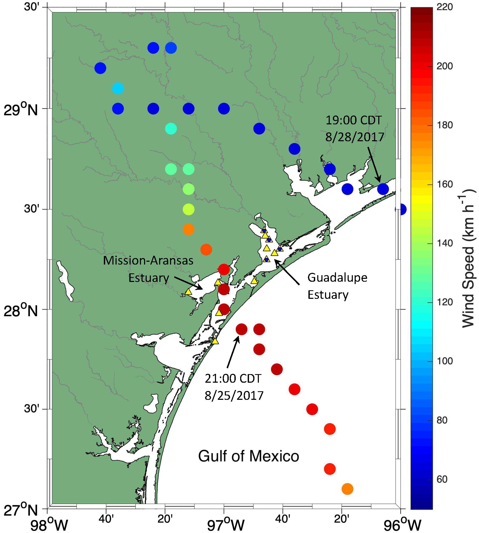
Figure 1. The track of Hurricane Harvey and wind speed (colorbar). The sampling stations in Mission-Aransas Estuary (MAE) and Guadalupe Estuary (GE) are shown in yellow triangles. The blue circles superimposed on the triangles in GE represent quarterly sampling stations (see text for details).

Harvey caused extensive destruction to coastal and inland communities and an economic loss of ∼$100 billion (Benfield, 2018). At the same time, it also offered an unprecedented opportunity for us to examine the effect of storm events on estuarine carbonate chemistry and CO₂ flux in the semiarid northwestern GOM coastal estuaries. This manuscript presents the temporal changes in the estuarine carbonate system and CO₂ flux as disparate post-Harvey influences were exemplified in the estuaries in the northwestern GOM, have similar geomorphic structure and physiography but receive freshwater from significantly different watersheds.

Materials and Methods

Study Area

Mission–Aransas Estuary and Guadalupe–San Antonio Estuary (GE) are both shallow lagoonal estuaries (1.5–2 m) in the south Texas coast (Montagna et al., 2013; Figure 1) with a diurnal tidal range of 12–15 cm (Evans et al., 2012; Ward, 2013). MAE includes three interconnected water bodies – Aransas Bay (primary bay) is connected to the GOM through the Aransas Ship Channel, Copano and Mesquite Bays are both secondary bays that are more directly affected by riverine input (Kim and Montagna, 2012). Mission and Aransas rivers discharge into Copano Bay, and Mesquite Bay receives water from the adjacent San Antonio Bay under flooding conditions. GE is adjacent to MAE to the north and includes Mission Lake, Hynes Bay, and San Antonio Bay, with the latter being the primary bay. The total area of San Antonio and Guadalupe watershed is 26,244 km² (GE) (Texas Water Development Board), much greater than that (4,821 km²) of Aransas and Mission rivers (MAE) (Mooney and McClelland, 2012). The GE watershed includes extensive urbanized areas and is considered eutrophic (Arismendez et al., 2009; Turner et al., 2014). In comparison, the MAE watershed has a small population and is mostly composed of agricultural/grass/shrub land, and MAE can be oligotrophic under low river discharge conditions (Evans et al., 2012).

Five long-term System Wide Monitoring Program (SWMP) stations in MAE were sampled from May 2014 on a bimonthly or monthly basis since May 2014 (Yao and Hu, 2017). Four stations have been sampled in GE from January 2014 on a quarterly basis (Montagna et al., 2018). However, starting from May 2017, bimonthly trips were carried out in GE until early December 2017 with an additional three stations (Figure 1). We focused on the observations made in 2017 but these results were also compared and contrasted with data from prior to 2017 (Yao et al., 2020).

Sample Collection

We followed the sample collection and analytical approaches outlined in McCutcheon et al. (2019) and Montagna et al. (2018) for sampling in GE. Briefly, a calibrated YSI 6920 multisonde was used to obtain in situ temperature, salinity, and dissolved oxygen (DO) concentration at both the surface (∼0.5 m) and the bottom (within 0.5 m from the sediment–water interface) of the water column, and a Van Dorn water sampler was used to take water samples from the surface and bottom. Following the standard OA sample collection and preservation protocol (Dickson et al., 2007), unfiltered water samples were collected into 250 mL borosilicate glass bottles for the lab analyses of total alkalinity (TA), total DIC, and pH. 100 μL saturated mercuric chloride (HgCl₂) was added into the sampling bottles and the bottle stoppers were sealed using Apiezon^® L grease, rubber band, and a hose clamp. Chlorophyll a and dissolved OC (DOC) samples from GE were preserved on ice until return to our shore-based lab for processing and analysis (Montagna et al., 2018). Field condition observations and carbonate chemistry sampling in MAE followed protocols in Yao and Hu (2017), and chlorophyll samples were collected using the same approach as that in the literature (Mooney and McClelland, 2012; Bruesewitz et al., 2013). No DOC samples were collected in MAE.

Chemical Analysis and Carbonate System Speciation Calculations

Total alkalinity was analyzed at 22 ± 0.1°C using Gran titration. DIC was analyzed using infrared detection. Both DIC and TA analyses had a precision of ±0.1%, and Certified Reference Material (CRM) was used throughout the sample analyses to ensure data quality (Dickson et al., 2003). Two approaches were taken to measure pH (Yao and Hu, 2017). Prior to mid September, 2017, pH for salinity <20 was measured using a calibrated high precision glass Orion^TM pH electrode, and the electrode was calibrated using three pH standards (4.01, 7.00, and 10.01); for samples with salinity ≥20, pH was measured using purified m-cresol purple with the method in Carter et al. (2013). The equation in Liu et al. (2011) was used in calculating pH values. After mid September 2017, a new equation (Douglas and Byrne, 2017) for wider salinity range (0–40, vs. 20–40 in the Liu et al.’s study) was used for the low salinity samples (<20) to replace the potentiometric measurement. All pH measurements were done at 25°C. Calcium concentration ([Ca²⁺]) was measured (from non-preserved water samples) using automatic titration on a Metrohm Titrando and ethylene glycol tetraacetic acid (EGTA) titrant, with a precision of ±0.02 mmol kg^–1.

Carbonate speciation calculations were conducted using the MatLab^® version CO2SYS program. Carbonic acid dissociation constants (K₁ and K₂) from Millero (2010) were used to account for the wide salinity range of the samples. Bisulfate dissociation constant was from Dickson (1990), and borate concentration was from Uppström (1974). Input variables for the speciation calculation were measured DIC and pH at 25°C. For this study we did not perform underway measurements due to logistical constraints. However, a 10-month time-series study conducted at the nearby Aransas Ship Channel revealed that the calculated CO₂ partial pressure (pCO₂) using discrete samples and those obtained by a calibrated SAMICO2 sensor (Sunburst^®) agreed within 15 μatm and an uncertainty of ∼30 μatm (McCutcheon et al., unpublished).

Chlorophyll and DOC analyses followed the protocols in Montagna et al. (2018) for the GE samples, and chlorophyll samples from MAE were analyzed using the method in Mooney and McClelland (2012). Data from MAE can be accessed through the Centralized Data Management Office of the National Estuarine Research Reserve Program¹.

CO₂ Flux Calculation

The air–water flux of CO₂ was calculated using Eq. 1:

$$F={\text{kK}}_0({\mathrm{pCO}}_{2,\mathrm{water}}-{\text{pCO}}_{2,\mathrm{air}})(1)$$

here k (m d^–1) is the gas transfer velocity calculated from wind speed (Jiang et al., 2008), K₀ (mol m^–3 atm^–1) is the gas solubility constant at in situ temperature and salinity (Weiss, 1974), pCO_2,water and pCO_2,air are partial pressure of CO₂ in surface water and the atmosphere, respectively. Wind speed data were downloaded from monitoring sites close to these estuaries https://tidesandcurrents.noaa.gov/map/index.shtml?type=MeteorologicalObservations&region=Texas and corrected to 10 m using the equation in Hsu et al. (1994). Positive F- value means CO₂ degassing to the atmosphere. pCO_2,air were calculated from:

$$p{\text{CO}}_{2,\mathrm{air}}=x{\text{CO}}_{2,\mathrm{air}}\times (P_{\text{b}}-P_{\text{w}})(2)$$

In Eq. 2, P_b (atm) is the barometric pressure from the weather stations in these two estuaries, P_w (atm) is the water vapor pressure calculated using salinity and temperature (Weiss and Price, 1980), and xCO_2,air (ppm) is the mole fraction atmospheric CO₂ in dry air. We did not measure air xCO₂ directly but chose to download monthly averaged xCO₂ data from http://www.esrl.noaa.gov/gmd/ccgg/trends. The area-weighted CO₂ flux in each estuary was calculated using the approach in Yao and Hu (2017) by separately calculating the fluxes in both the primary and secondary bays and then integrating them together.

Results

River Discharge Into MAE and GE

Daily mean river discharge data were obtained from the United States Geological Survey² (Figure 2A) from the beginning of our sampling period till April 2018. Three gauges (Aransas River – 08189700 and Mission River – 08189500 for MAE and Guadalupe River – 08188810 for GE) were used here. Note the Guadalupe gauge measures combined input of both San Antonio and Guadalupe rivers as the former merges with the latter before reaching this gauge.

FIGURE 2

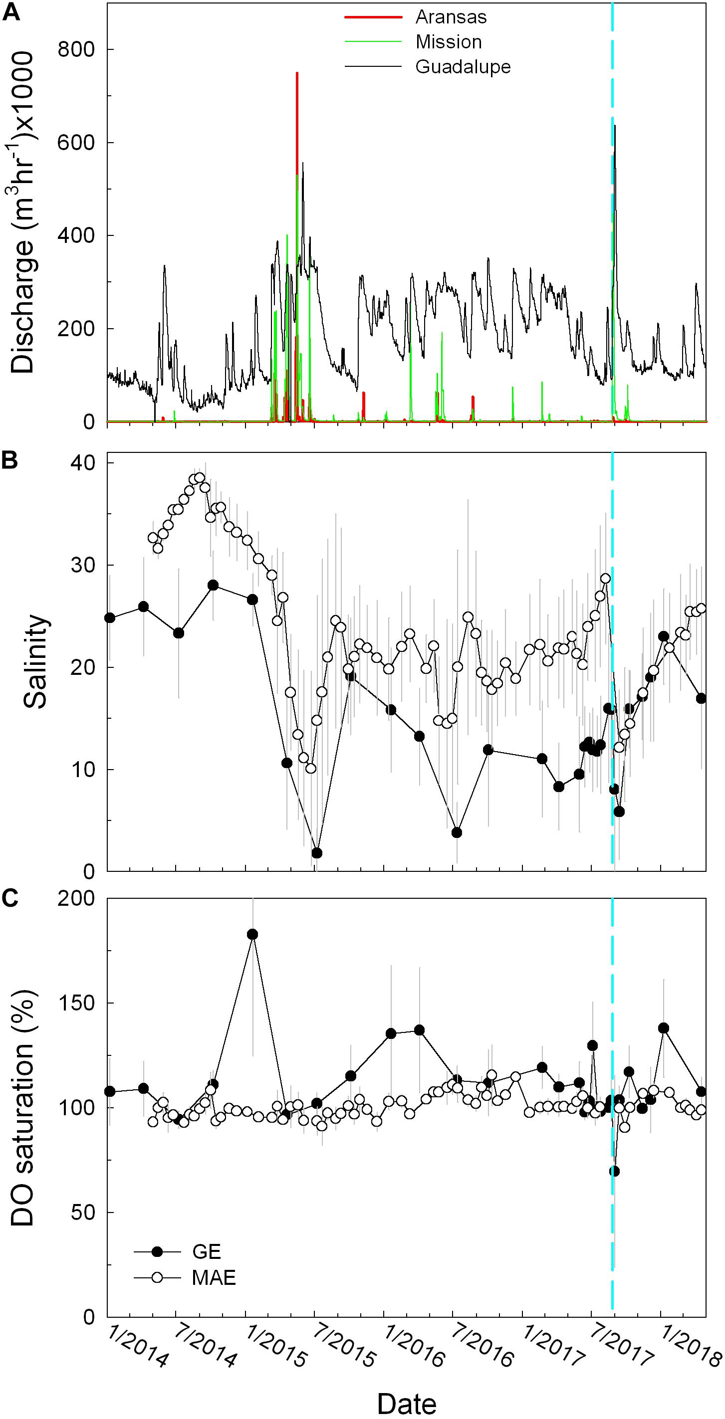
Figure 2. (A) Discharge of Aransas (red), Mission (green), and Guadalupe (black) rivers. (B) Average salinity in MAE (open circles) and GE (closed circles). (C) Percent saturation of dissolved oxygen. The gray vertical lines represent standard deviation of the mean. The cyan dashed lines (and in figures hereafter) represent the date (August 25, 2017) on which Hurricane Harvey made landfall.

Compared to Guadalupe River that had continuous freshwater discharge, both Aransas and Mission rivers had low discharge during most of the study period (Figure 2A). One month prior to Harvey, Aransas, Mission, and Guadalupe (from south to north) rivers had the average hourly discharge rates of 0.2 ± 0.1, 0.1 ± 0.6, and 120.6 ± 50.5 × 10³ m³ h^–1, respectively. Hurricane precipitation-induced increase in river discharge started to be observed on August 26 in Aransas River (2.2 × 10³ m³ h^–1), in which the discharge peaked on August 27 (9.7 × 10³ m³h^–1) and quickly returned to the baseline rate in 15 days. Mission River had near zero freshwater discharge prior to the hurricane although the value rapidly increased to 217.1 × 10³ m³ h^–1 on August 26 and peaked on August 28 (446.5 × 10³ m³ h^–1). After half a month, its discharge was still 5.7 × 10³ m³ h^–1, significantly greater than the baseline level prior to Harvey. In comparison, Guadalupe River saw an increase in discharge from August 26 although the peak (637.1 × 10³ m³ h^–1) appeared several days later on September 1. Notably, each of the rivers had a secondary peak discharge at the end of September to early October (Figure 2A). For example, Aransas River had 5.0 × 10³ m³ h^–1 (September 28), Mission River had 32.8 × 10³ m³ h^–1 (September 29), and Guadalupe River had 217.1 × 10³ m³ h^–1 (October 4), possibly due to intermittent rainfall through the month of September, in addition to the direct Harvey influence.

If accounting for the secondary discharge peaks till the middle of October (i.e., October 15), when all river discharges returned to their respective low levels prior to the hurricane, the three rivers had exported 1.2 × 10⁶ (Aransas), 5.3 × 10⁷ (Mission), and 3.0 × 10⁸ (Guadalupe) m³ freshwater since Harvey made landfall.

Changes in Estuarine Hydrography

Because of the shallow depths in these two estuaries, both GE and MAE usually had little stratification except under flooding conditions. For example, salinity difference between bottom and surface (ΔS) in GE was 2.2 ± 3.4 and 0.7 ± 1.7 in MAE across all sampling stations in our multiyear surveys (2014–2018). Prior to Harvey (August 23), surface salinity in GE ranged from 5.7 at close to the Guadalupe River mouth to 20.0 in lower GE with ΔS as much as 6.9 in the latter (2 m depth). A few days after Harvey made landfall (September 1), salinity at the station close to the river mouth decreased to near zero (0.2) at both surface and bottom, and surface water at all other stations decreased to 0.3–5.5, while bottom water salinity decreases were small (up to 6.0) compared to the values prior to the hurricane, with a range of 9.7–20.9. In mid-September (September 13), continued salinity decrease in bottom water was observed (ranging from 1.2 to 13.9) while surface salinity remained similar to September 1, suggesting continued river input and mixing that was flushing salt out of GE. Afterward (October 9), the entire GE returned to pre-Harvey salinity with little surface-bottom stratification (ΔS<2). In comparison, slight stratification (ΔS∼2–3) was observed in the upper MAE (i.e., the two stations in Copano Bay) on August 8 with the surface salinity of 20.8–20.9 and the rest of MAE was vertically well-mixed, with a salinity range of 27.2–36.4 from mid-MAE to Aransas Ship Channel. In mid-September (September 13), the entire MAE had significant decrease in salinity (6.8–22.2) although stratification was still minimal (ΔS<1.5) except at the station located in Aransas Bay (ΔS = 6.8). However, because MAE was in a state of drought several months prior to Harvey, post-Harvey salinity increased but remained relatively low compared to pre-Harvey months (Figure 2B).

In addition to the hurricane-induced strong river discharge in 2017, significant precipitation caused high river discharge in all three rivers and led to prior episodes of estuarine freshening (June–July 2015, Figures 2A,B). For example, salinity in GE was as low as 1.8 ± 2.4 on July 8, 2015 and that in MAE was 10.1 ± 9.5 on June 23, 2015, both of which were lower than the values observed after Harvey. A smaller decrease in salinity was also observed in both estuaries in mid-2016 (Figure 2B). We recognize that the comparison based on the “snapshots” of sampling events could be overly simplified and the observations were tied to the timing of the field trips. However, the overall greater river discharges in the two non-hurricane years did suggest greater estuarine freshening in these earlier years (Figure 2A).

Average DO saturation (%DO) in GE surface water was 108.2 ± 23.7% and bottom water was 93.8 ± 27.1%. In MAE, these values were 100.6 ± 6.7 and 98.8 ± 8.6%, respectively (Figure 2C). MAE did not experience substantial DO decrease throughout our sampling period, while discrete sampling suggested that GE had hypoxic conditions in the upper estuary on September 1, 2017, and the hypoxic condition in the station closest to the river mouth persisted for about a week with continued freshwater input that kept salinity low (Walker et al., unpublished).

Carbonate System Parameters

Both GE and MAE had fairly high TA and DIC levels throughout the sampling period (i.e., 2832 ± 315 and 2560 ± 293 μmol kg^–1 for GE and 2539 ± 161 and 2271 ± 146 μmol kg^–1 for MAE, respectively), mostly greater than the ocean water values in the northwestern GOM (Hu et al., 2018). At the same time, their pH values were generally higher than (8.151 ± 0.234 in GE) or equivalent (8.078 ± 0.079 in MAE) to the open ocean values.

TA and DIC had already started to decline in both estuaries from early June 2017. Harvey-induced freshwater input further pushed both TA and DIC to their respective minima, i.e., TA = 2186 ± 92 μmol kg^–1 and DIC = 2154 ± 143 μmol kg^–1 in GE (September 1), and TA = 2108 ± 240 μmol kg^–1 and DIC = 1918 ± 199 μmol kg^–1 in MAE (September 13) (Figures 3A,B). pH in MAE did not change much before and after Harvey, i.e., from 8.002 ± 0.043 on August 8 to 8.077 ± 0.108 on September 13. However, a significant pH decline in GE was observed, i.e., pH prior to Harvey was 8.019 ± 0.191 (August 23), several days after Harvey pH dropped significantly (7.521 ± 0.191 on September 1) but then increased again to 7.914 ± 0.212 when both TA and DIC concentrations increased (September 13) (Figure 3C). [Ca²⁺] mostly followed salinity throughout our sampling period (Figure 3D) although the regression between [Ca²⁺] and salinity offered more insights on the river endmember composition changes at different hydrologic conditions (see the section “Discussion” for more details).

FIGURE 3

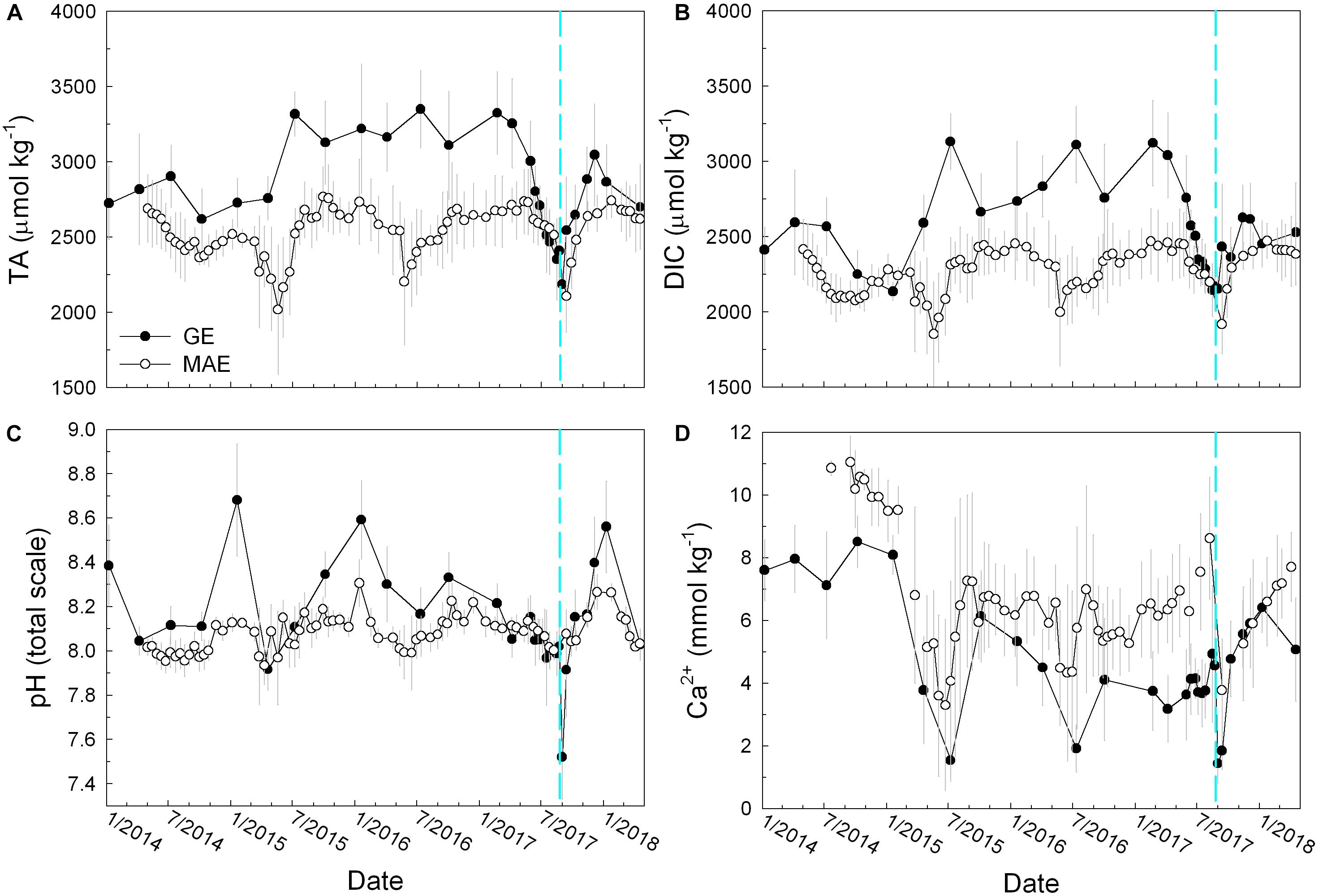
Figure 3. Temporal distributions of (A) total alkalinity (TA), (B) total dissolved inorganic carbon (DIC), (C) in situ pH on total scale, and (D) calcium ion concentration ([Ca²⁺]). The open circles represent MAE and the close circles represent GE.

Compared to hurricane-induced estuarine carbonate system changes, the period of freshwater discharge increase in mid-2015 caused similar changes to TA and DIC in MAE as those after Harvey, although GE experienced elevated TA and DIC concentrations (Figures 3A,B) instead of the large decrease after Harvey.

CO₂ Partial Pressure, Normalized pCO₂, and Air–Water CO₂ Flux

Surface water pCO₂ in GE exhibited much more temporal variability than in MAE (Figure 4A), i.e., 666 ± 702 (GE) vs. 477 ± 84 μatm (MAE). Following Harvey, pCO₂ in GE increased significantly compared to the background values and reached 3940 ± 2423 μatm (September 1), although the value quickly decreased to near background level 372 ± 40 μatm in slightly greater than a month (October 9). It is worth noting that even though river discharge in mid-2015 (Figure 2A) led to more freshening of both estuaries, pCO₂ in GE then was much lower (1278 ± 472 μatm, Figure 4A) than the post-Harvey conditions; whereas MAE did not exhibit significant variations in pCO₂ before and after Harvey (pCO₂ was always around 450–550 μatm). In comparison, pCO₂ increased slightly from the drought period in mid-2014 to early 2015 (Yao and Hu, 2017).

FIGURE 4

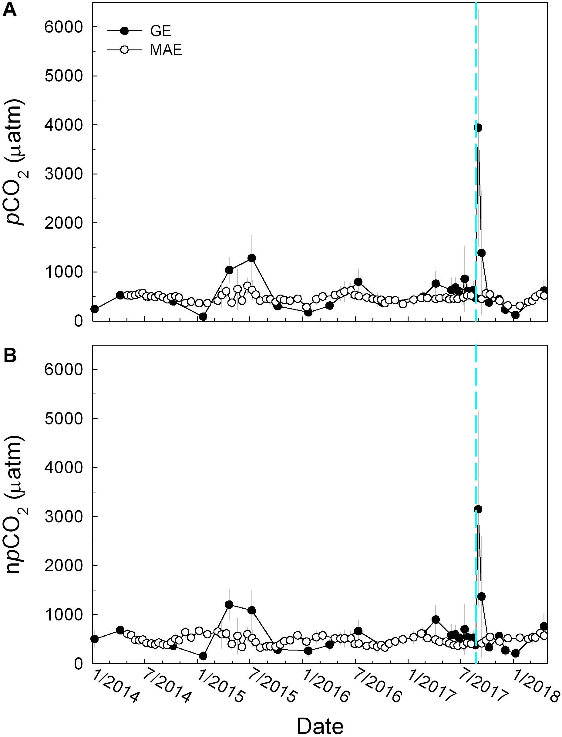
Figure 4. Temporal distributions of (A) in situ pCO₂ and (B) temperature normalized pCO₂ (npCO₂) in MAE (open circles) and GE (closed circles), see text for the temperatures that data from these two estuaries were normalized to. The gray vertical lines represent standard deviation of the mean.

To remove the temperature effect on pCO₂ variation, surface water pCO₂ was normalized (npCO₂) based on the respective average temperatures of the two estuaries, i.e., 25.9°C in GE and 24.4°C in MAE, following the scheme in Takahashi et al. (2002), also see Yao and Hu (2017). Similar to pCO₂, npCO₂ showed the maximum values after Harvey (3147 ± 1365 μatm on September 1, Figure 4B), and despite the higher freshwater influence in mid-2015, npCO₂ at that time was much lower at the 1100–1200 μatm level.

As defined in Eq. 1, CO₂ flux is a function of wind speed (gas transfer) and air–water pCO₂ gradient. Contrary to the pCO₂ values (Figure 4A), the post-Harvey maximum pCO₂ in GE did not translate into the highest CO₂ efflux in our study period (164 ± 122 mmol m^–2 d^–1 on September 1, 2017). Instead, the highest calculated CO₂ efflux occurred in mid-2015 (181 ± 100 mmol m^–2 d^–1 on July 8, 2015) (Figure 5A), and the wind speed 9.3 m s^–1 on the 2015 observation date was much higher than the post-Harvey date (3.6 m s^–1) (Figure 5B). In comparison, MAE did not exhibit significant changes in CO₂ flux before and after the hurricane (Figure 5A).

FIGURE 5

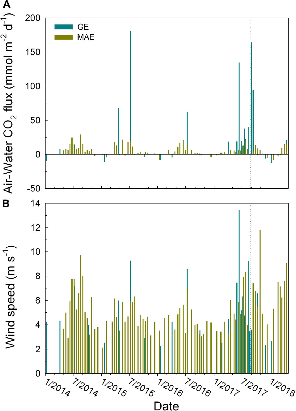
Figure 5. Temporal distributions of (A) air–water CO₂ flux (unit mmol m^–2 d^–1) and (B) daily wind speed on the sampling days in GE (dark green) and MAE (dark yellow). The dotted lines represent the date (August 25, 2017) on which Hurricane Harvey made landfall.

Chlorophyll a and DOC

Both GE and MAE experienced various extents of changes in chlorophyll concentration throughout our study period although the magnitudes of changes were quite different. Chlorophyll concentration in GE showed significantly greater temporal changes that corresponded to the magnitude of freshwater input than MAE, i.e., higher freshwater discharge in both 2015 and 2016 appeared to coincide with elevated chlorophyll concentration (Figures 2A, 6). After Harvey, chlorophyll concentration reached an all-time minimum (4.9 ± 1.3 μg L^–1) on September 8 (Figure 6) and this value rebounded to 19.8 ± 8.6 on September 13, the same level as that prior to Harvey (August 16). In addition, the chlorophyll minimum coincided with the DOC maximum (September 8) and the two parameter exhibited a significant negative correlation (p = 0.03).

FIGURE 6

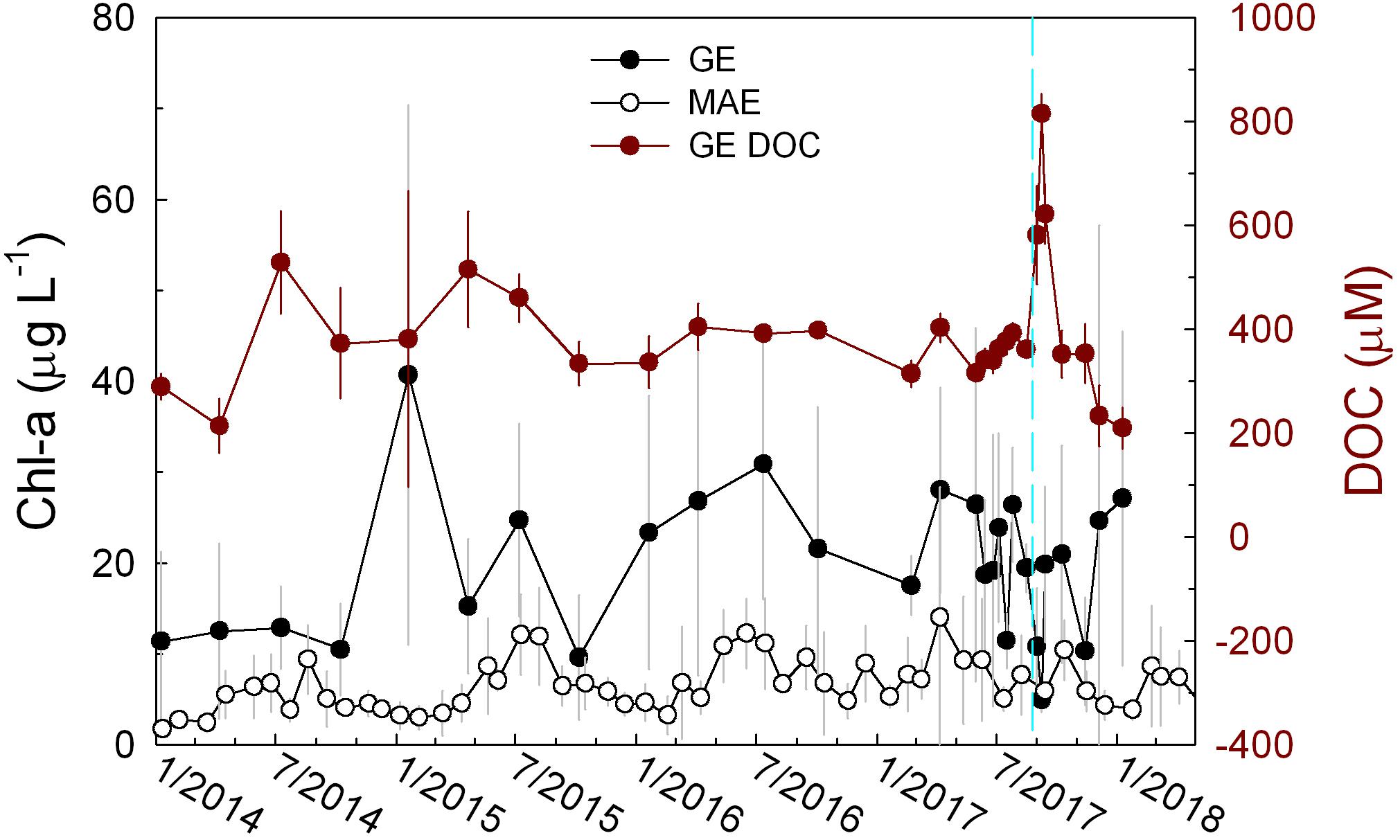
Figure 6. Temporal distributions of chlorophyll a concentration in both GE and MAE. DOC from GE is shown in brown circles.

Discussion

Tropical storms including hurricanes are capable of mobilizing large amounts of terrestrial carbon and nutrients, facilitating their transport across the land–ocean boundary, and at the same time, enhancing sediment resuspension that exposes buried organic matter to oxic conditions for increased microbial respiration; hence, significantly influencing estuarine and coastal carbon cycle (Crosswell et al., 2014; Majidzadeh et al., 2017; Lemay et al., 2018; Paerl et al., 2018; Van Dam et al., 2018; Letourneau and Medeiros, 2019; Osburn et al., 2019). On the other hand, few studies have examined inter-system variabilities and compared the hurricane effect with smaller scale flooding events. Our continuous sampling before and after Harvey provided an opportunity to examine these variabilities.

Spatial Heterogeneity in Estuarine Responses to Hurricane Influence

It is well known that estuaries along the northwestern GOM coast receive decreasing river discharge from northeast to southwest, and at the same time, these estuaries have a gradient of decreasing freshwater balance, i.e., freshwater input minus evaporation (Montagna et al., 2013). GE received much more freshwater than MAE (Figure 2A) and the river flow has been continuous despite its temporal changes over time. In comparison, the two rivers that empty into MAE frequently experienced near zero net flow, and conspicuous discharge only appeared intermittently (Figure 2A) corresponding to local/regional precipitation. As a result, prior to Harvey, salinity in MAE (28.7 ± 6.4) was substantially higher than in GE (15.8 ± 5.7) (Figure 2B). However, both TA and DIC have been showing a decreasing trend since April 2017 (Figures 3A,B) leading up to the hurricane as salinity in both estuaries increased (Figure 2B). The TA and DIC decreases were mainly caused by the increasing presence of seawater in these estuaries, as seawater has lower levels of TA and DIC but higher [Ca²⁺] than the freshwater endmembers (Figure 3D; Hu et al., 2015).

After Harvey made landfall on August 25, 2017, GE first experienced an ephemeral (hours) storm surge that brought high salinity water to the innermost station where an in situ monitoring sonde (for salinity and DO) was in place (Walker et al., unpublished). Half a month after the hurricane, GE and MAE both experienced large decreases in salinity compared with data collected prior to the hurricane (Figure 2B). However, TA/DIC ratio in these two estuaries behaved differently before and after the storm, i.e., greater decreases in GE (from 1.11 ± 0.04 and 1.02 ± 0.03) than those in MAE (from 1.14 ± 0.02 to 1.10 ± 0.03), indicating GE became much more enriched in CO₂ (see below for further discussion). This excess CO₂ was then responsible for the much lower pH (Figure 3C) and higher pCO₂ in GE (Figure 4A). In MAE, however, the similar extent (∼13–16%) of TA and DIC dilution before and after Harvey did not result in large changes in estuarine carbonate speciation in MAE. Hence, neither pH nor pCO₂ varied substantially.

The similarity (i.e., freshwater discharge induced estuarine freshening) and contrast (i.e., difference in carbonate speciation after Harvey) reflected spatial heterogeneity of hurricane influence on coastal estuaries, even though these estuaries are spatially close to each other. Precipitation caused by Harvey was mostly concentrated in the Houston area in the north and decreased to the south (this study area) and east along the coast (van Oldenborgh et al., 2017). Therefore, even though the center of the hurricane passed right through MAE (Figure 1), precipitation and the resulted river discharge there was lower than in GE. For example, integrated freshwater input into GE from August 26 to September 13, when the minimum salinity was observed, was 3.6 times of that into MAE (1.59 × 10⁸ vs. 0.45 × 10⁸ m³). The greater amount of freshwater input into GE also should stem from its much larger watershed area. Considering that the two estuaries have similar total volume (Montagna et al., 2013), freshwater thus caused more extensive flushing in GE than in MAE (also see Solis and Powell, 1999). The faster salinity change (i.e., first decrease and then increase) in GE than in MAE, which tends to remained freshened for prolonged period (Orlando et al., 1993), also indicated relatively more efficient water exchange with the coastal ocean in GE (Figure 2B).

In addition to the difference in the amount of freshwater input, apparently the characteristics of the freshwater coming into these estuaries were different between the two estuaries. While MAE did not exhibit significant changes in chlorophyll level after the storm (Figure 6), GE had large increase in DOC concentration (Figure 6) along with freshening of the entire estuary (Figure 2B) and decrease in overall DO (Figure 2C) chlorophyll levels (Figure 6), the latter was probably caused by increases in water turbidity that inhibited estuarine primary production. In fact, the in situ sonde at the innermost station in GE revealed a week-long hypoxic condition after the hurricane till 3–4 days before our post-Harvey field sampling on September 13 (Walker et al., unpublished). The high OC input as a result of hurricane activity might have prompted extensive suboxic to anoxic conditions in GE due to high rates of metabolic reactions.

High post-Harvey DOC levels have been observed in other storm-perturbed estuarine systems in which CO₂ production is enhanced (Van Dam et al., 2018; Osburn et al., 2019). Similarly, the excess OC input into GE was consistent with the observed high pCO₂ levels (Figures 3D, 4A).

Temporal Heterogeneity in Estuarine Carbonate System in Response to Storm-Induced Freshwater Input

Not only did the estuaries respond to hurricane-induced freshwater discharge differently, even though they are closely located in a narrow geographic range, within each estuary the responses were also different at different times. There were two occasions of large pulses of freshwater input into both estuaries, i.e., June–July 2015 and the similar period in 2016, with the 2015 flooding event having higher amount of freshwater discharge and lower salinity in these estuaries compared to the post-Harvey conditions (Figures 2A,B). Nevertheless, the patterns for MAE have been rather consistent between “normal” flooding conditions and that after Harvey, i.e., both TA and DIC appeared being “diluted” at each of the salinity minima (Figures 3A,B) with modest increase in pCO₂ (by <100 μatm on average, Figure 4A) but virtually unchanged pH (Figure 3C, also see Yao and Hu, 2017). However, water chemistry in GE exhibited different behaviors when encountering significant increase in river discharge. For example, following a drought in south Texas prior to mid-2015, the large increase in river discharge elevated both TA and DIC concentrations in GE, and the highest concentrations corresponded to the lowest salinity (Figures 2B, 3A,B). Then again in mid-2016, another lesser extent of river input also increased both TA and DIC. The increase in river influence following river flooding can also be viewed using the time-series of the intercept of Ca²⁺ vs. salinity linear regression ([Ca²⁺]₀, Figure 7) as Ca²⁺ concentration often exhibited excellent linear relationship with salinity hence [Ca²⁺]₀ can be used to infer river water Ca²⁺ concentration. During the 2015 and 2016 flooding periods, [Ca²⁺]₀ values for GE were 1.25 and 1.18 mmol kg^–1, respectively (Figure 7A). Because of relatively narrow range of calcium ion to TA ratios in Guadalupe and San Antonio Rivers (Ca²⁺:TA = 0.42 ± 0.05, Texas Commission on Environmental Quality), river alkalinity was estimated to be in the range of 2800–3000 μmol kg^–1. This high riverine TA thus can explain the high TA values in 2015 and 2016 (Figure 3A). In comparison, [Ca²⁺]₀ was 0.74 mmol kg^–1 on August 23 (prior to Harvey) and 0.87 mmol kg^–1 on September 1 (Figure 7C), despite the fact that salinity has decreased from 15.8 to 8.1 on the latter date (Figure 2B). The nearly invariant [Ca²⁺]₀ suggested that initial Harvey-induced freshwater input into GE was low in weathering products, likely a result of local precipitation and runoff from adjacent area around GE. Similarly, the post-Harvey samples in MAE suggested the estuarine water was mostly diluted by precipitation because [Ca²⁺]₀ decreased from 1.39 mmol kg^–1 on August 8 (prior to Harvey) to 0.37 mmol kg^–1 on September 13 (Figure 7D). After the initial dilution period, GE started receiving river waters with substantially higher levels of weathering products as indicated by the large increase in the [Ca²⁺]₀ value (Figure 7C), although that for MAE remained relatively low (0.6–0.7 mmol kg^–1) through December 2017, suggesting that watershed that contributed to GE continued moving high levels of weathering products downstream while MAE watershed did not have high levels of these solutes thus precipitation-led dilution dominated the post-Harvey months. It is worth noting that the Ca²⁺ vs. salinity regression is not reliable for predicting river endmember under drought conditions, as MAE in much of 2014 (Figure 7B) exhibited a reverse estuary pattern with the upper estuary having greater salinity due to net evaporation (see Yao and Hu, 2017); hence, the regressed intercept became negative, a physically impossible freshwater endmember.

FIGURE 7

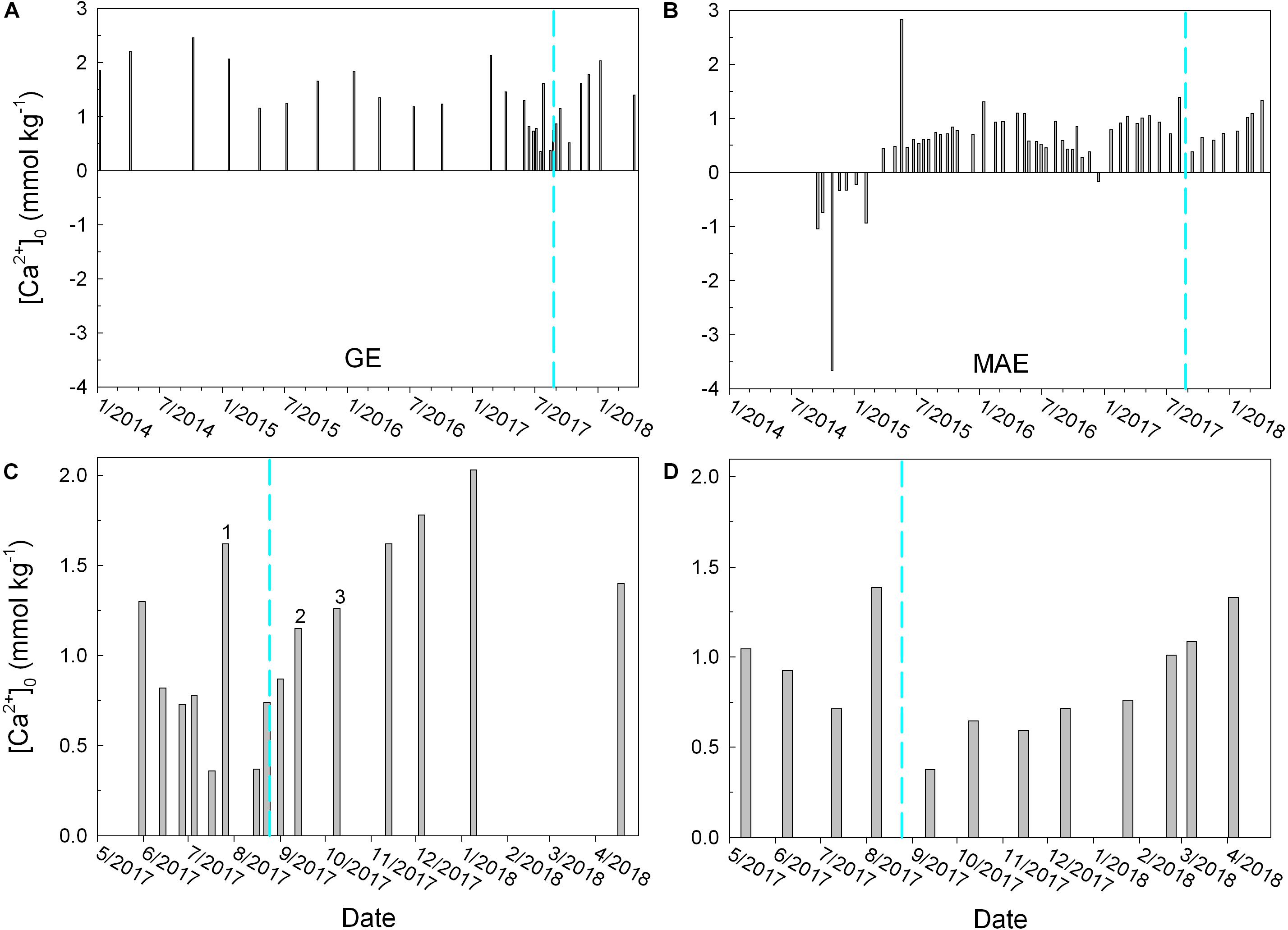
Figure 7. Temporal changes in the intercept of [Ca²⁺] and salinity regression (i.e., [Ca²⁺]₀) in both GE (A) and MAE (B). Panels (C) and (D) show the data during the period of May 2017 to April 2018 for these estuaries, respectively. Other than the marked [Ca²⁺]₀ bars that have regressed r² values of 0.75 (#1, July 26), 0.80 (#2, September 13), and 0.95 (#3, October 9), all other r² values in (C) and (D) are better than 0.98. The lower r² values were all due to one data point that did not fall on each regression line possibly due to the significantly varying river endmember on the time scale of estuarine mixing (Cifuentes et al., 1990).

The immediate post-Harvey increase in pCO₂ was much larger than those from the two prior flooding periods (Figure 4A) and it was also higher when the values were normalized to the same temperature (npCO₂, Figure 4B). Based on the comparison between the prior flooding event and post-Harvey, it appeared that the hurricane and its associated freshwater input were able to mobilize OC from the lower reaches of Guadalupe/San Antonio rivers, which then fueled strong microbial respiration through physical disturbance to the watershed (Paerl et al., 2018), compared to regular river flooding caused by large scale precipitation (Figure 8), even though the latter could lead to higher amount of freshwater input into GE. On the other hand, such elevated high CO₂ condition was rather short-lived (∼1 month). The high levels of weathering product coming off the upper reaches of the rivers (Figure 7C) that contributed to GE, along with rebounding estuarine primary production as indicated by the increase in chlorophyll levels (Figure 6), should have provided much buffer.

FIGURE 8

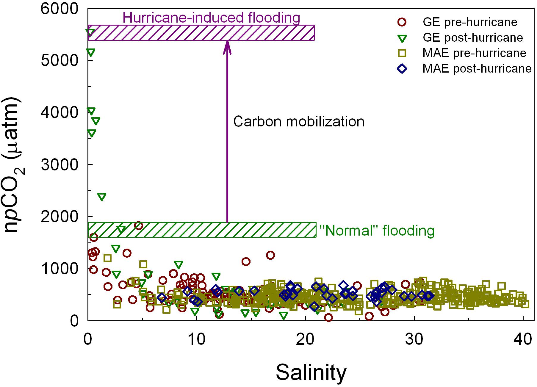
Figure 8. A comparison of temperature normalized pCO₂ (npCO₂) from before and after Hurricane Harvey. The difference between the maximum npCO₂ values from pre-Harvey flooding periods and that from post-Harvey is considered to be CO₂ signal generated from hurricane mobilized carbon.

Air–Water CO₂ Flux

Despite the rarity of studies that investigate hurricane influence on estuarine CO₂ fluxes, hurricanes and strong storms are known to significantly increase this flux. For example, Crosswell et al. (2014) observed that CO₂ fluxes in the eutrophic Neuse River Estuary and Pamlico Sound were both −2.4 mmol m^–2 d^–1 prior to Hurricane Irene (2011). These two water bodies experienced significant CO₂ efflux during the storm period (i.e., 4080 and 384 mmol m^–2 d^–1, respectively), then the fluxes decreased to 154 and 7 mmol m^–2 d^–1 17 days after Irene, respectively. While directly enhanced CO₂ flux was mainly due to strong wind forcing that facilitates OC remineralization caused by physical mixing and sediment resuspension when a hurricane directly passes over (Crosswell et al., 2014), the 2015 Hurricane Joaquin did not make landfall but induced continental flooding in the same region, and this storm event also elevated estuarine CO₂ flux (Van Dam et al., 2018). CO₂ fluxes during the flooding period (62 and 265 mmol m^–2 d^–1) were found to be 3.6 and 15.6 times of those prior to the flood in Neuse River and New River estuaries, respectively.

Compared to these east coast studies, we did not have data during Harvey except the single bottom water monitoring station (Walker et al., unpublished). However, the post-Harvey CO₂ flux in GE increased from the pre-hurricane near neutral levels (−0.2 ± 5.0 mmol m^–2 h^–1) to 164 ± 122 mmol m^–2 h^–1 on September 1 and then 94 ± 161 mmol m^–2 h^–1 on September 13, both were greater than post-storm CO₂ flux observed in the east coast estuaries (Crosswell et al., 2014; Van Dam et al., 2018). In comparison, post-Harvey CO₂ flux in MAE (4 ± 3 mmol m^–2 d^–1) was much lower but on par with those values obtained from those east coast estuaries. The reason for such distinct difference in CO₂ flux may be explained by the different extents of nutrient pollution that these estuaries experienced (see below).

In fact, despite that observed pCO₂ (hence water–air pCO₂ gradient) was the largest in GE after Harvey, water-to-air CO₂ flux was not the highest at that time (Figure 5A). The difference mainly stemmed from the higher gas transfer velocity in 7.8 m d^–1 (at wind speed 9.3 m s^–1) on the sampling day in mid-2015 vs. 1.9 m d^–1 (at wind speed 3.6 m s^–1) after Harvey.

Overall, water-to-air CO₂ flux during the 1-month period after Harvey (August 27–September 26, 2017) was estimated to be 1.6 × 10⁹ mol. Integrating the 2017 flux values to the whole year the CO₂ efflux in GE in 2017 was 4.7 × 10⁹ mol. Therefore, this 1-month period accounted for ∼35% annual CO₂ emission in that year, and this estimate should represent a lower limit because CO₂ flux could have been higher during the storm due to much higher gas transfer velocity and potential sediment resuspension in this shallow estuary. In comparison, much sparser measurements in 2015 and 2016 suggested that the flood-induced CO₂ emission accounted for 78 and 132% of annual values, respectively. Note all calculated CO₂ flux values were negative in 2016 except that from the flooding period that year. Considering the limited observations in these 2 years and that both river discharge and wind speed both played an important role in controlling CO₂ flux, these two estimates thus probably had high uncertainties.

CO₂ flux in MAE during the 2015 and 2016 flooding periods reached as much as 21–22 mmol m^–2 d^–1, much greater than that from the post-Harvey value. Furthermore, the latter flux from August 26 to September 25 (6.6 × 10⁷ mol) was not only much smaller than the GE values, but also appeared not extraordinary in the integrated annual CO₂ flux (close to monthly mean of 5.0 × 10⁷ mol), although again the CO₂ flux during the storm is unknown so this value can only be considered as a conservative estimate.

Post-Harvey freshwater input into MAE was less than that from the 2015, and that sedimentary total OC (TOC) content in MAE is <0.2% (Souza et al., 2012), which is much lower than that in the eutrophic system in the east coast (1.3–7.5%, see Cooper et al., 2004) where enhanced OC remineralization following sediment resuspension was attributed to large CO₂ fluxes during the storms (Crosswell et al., 2012). It is therefore unlikely that CO₂ flux in MAE during Harvey was much larger than the values from the flooding period in 2015 and 2016 because of low sedimentary carbon content and the extent that resuspended OC can stimulate respiration. Similarly, TOC concentration in GE sediment is ∼0.65% (Trefry and Presley, 1976), also suggesting the sediment resuspension and subsequent remineralization probably was not as large a CO₂ source hence flux as in the east coast estuaries, despite that fact that GE was more eutrophic than MAE (for example, the higher overall chlorophyll levels, Figure 6). Nevertheless, to obtain accurate quantification of CO₂ flux in these dynamic estuaries, especially those that are affected by irregular freshwater input such as these in the semiarid environments, higher frequency and sustained measurements than what is presented here are needed.

Conclusion

This is the first study that examined carbonate chemistry and CO₂ flux as a result of a major hurricane in the semiarid northwestern GOM coast. The two studied estuaries are next to each other and have similar geomorphic structure and physiography, yet the watershed areas of major contributing rivers differ by five times. In addition, MAE in the south mostly experienced wind forcing with smaller freshwater input, while GE in the north received much larger freshwater input from a much greater expanse of watershed. Therefore, both water column carbonate chemistry and air–water CO₂ flux exhibited different behaviors. MAE mostly reflected a dilution effect (for TA and DIC) with limited changes in pH and CO₂ flux after Harvey, while GE first showed dilution accompanied by enhanced respiration and short-lived low oxygen conditions, which was followed by large input of river water enriched in TA and DIC and elevated primary production that helped to buffer the acidified conditions (low pH and high pCO₂) after Harvey.

Because of the different behaviors in pCO₂ and wind conditions, GE experienced significant increase in CO₂ efflux that was disproportionally larger than average monthly CO₂ flux in this estuary, yet MAE did not exhibit significant change in CO₂ flux as a result of the hurricane. However, when the post-Harvey CO₂ flux was compared with prior flooding events in these estuaries, the CO₂ efflux cause by hurricane influences may not be necessarily larger. Instead, flooding in the past that was not associated with strong storms such as Harvey may have caused more CO₂ emission in these estuaries, as respiration based on sediment resuspension liberated OC may not be as significant as in the eutrophic estuaries in the U.S. east coast, given the much lower sedimentary OC contents in our studied estuaries.

Nevertheless, we recognize that the relatively small hurricane influence on estuarine CO₂ flux was dependent on the assumption that this flux during the hurricane did not differ significantly from the observations after the storm, mainly based on the lower sediment OC contents than the much more eutrophic U.S. east coast estuaries. However, to better constrain this flux term, which is exceedingly dynamic in the semiarid environment, sustained observations in conjunction with high resolution monitoring are needed.

Data Availability Statement

Data used in this manuscript can be accessed through BCO-DMO repository (https://www.bco-dmo.org/dataset/784673).

Author Contributions

CS, HY, MM, and LW conducted the field sampling and laboratory analyses. XH designed this study, performed the data analysis, and worked with HY on CO₂ flux calculations and with MW on interpreting dissolved organic carbon and chlorophyll a data. XH wrote the manuscript and other authors participated in the discussions and finalized the manuscript.

Funding

This study was funded by the National Science Foundation (NSF) Chemical Oceanography Program (OCE-1760006 and OCE-1654232). Earlier sampling has been supported by NOAA’s NOS National Center for Coastal Ocean Science (Contract No. NA15NOS4780185) and the Texas Research Development Fund from the Research and Commercialization Office of Texas A&M University – Corpus Christi, respectively.

Conflict of Interest

The authors declare that the research was conducted in the absence of any commercial or financial relationships that could be construed as a potential conflict of interest.

Acknowledgments

We are grateful for the fieldwork assistance provided by the staff and students at both the Mission Aransas National Estuarine Research Reserve (NERR) and the University of Texas Marine Science Institute. We also thank R. Kalk, L. Hyde, and E. Morgan in P. Montagna’s Lab as well as K. Hayes in MW’s Lab for their help with field sampling and logistics in Guadalupe Estuary. The MAE research was supported in part by operations grants to the Mission–Aransas National Estuarine Research Reserve from the Office of Coastal Management, National Oceanic and Atmospheric Administration. System-Wide Monitoring Program data were collected by the research staff of the Mission–Aransas NERR and hosted by the Central Data Management Office of the National Estuarine Research Reserve System. The two reviewers provided constructive comments, which helped to improve the quality of this work.

Footnotes

1. ^ http://cdmo.baruch.sc.edu/
2. ^ https://waterdata.usgs.gov/nwis

References

Abril, G., Etcheber, H., Borges, A. V., and Frankignoulle, M. (2000). Excess atmospheric carbon dioxide transported by rivers into the Scheldt estuary. Comptes Rendus de l’Académie des Sci. - Series IIA - Earth Planet. Sci. 330, 761–768. doi: 10.1016/s1251-8050(00)00231-7

CrossRef Full Text | Google Scholar

Arismendez, S. S., Kim, H.-C., Brenner, J., and Montagna, P. A. (2009). Application of watershed analyses and ecosystem modeling to investigate land–water nutrient coupling processes in the Guadalupe Estuary Texas. Ecol. Inform. 4, 243–253. doi: 10.1016/j.ecoinf.2009.07.002

CrossRef Full Text | Google Scholar

Bauer, J. E., Cai, W.-J., Raymond, P. A., Bianchi, T. S., Hopkinson, C. S., and Regnier, P. G. (2013). The changing carbon cycle of the coastal ocean. Nature 504, 61–70. doi: 10.1038/nature12857

PubMed Abstract | CrossRef Full Text | Google Scholar

Benfield, A. (2018). Weather, Climate and Catastrophe Insight: 2017 Annual Report. (Aon Rep. GDM05083). London: AON.

Google Scholar

Borges, A. V., Ruddick, K., Schiettecatte, L. S., and Delille, B. (2008). Net ecosystem production and carbon dioxide fluxes in the Scheldt estuarine plume. BMC Ecol. 8:15. doi: 10.1186/1472-6785-8-15

PubMed Abstract | CrossRef Full Text | Google Scholar

Borges, A. V., Schiettecatte, L. S., Abril, G., Delille, B., and Gazeau, F. (2006). Carbon dioxide in European coastal waters. Estuar. Coast. Shelf Sci. 70, 375–387. doi: 10.1016/j.ecss.2006.05.046

CrossRef Full Text | Google Scholar

Bruesewitz, D. A., Gardner, W. S., Mooney, R. F., Pollard, L., and Buskey, E. J. (2013). Estuarine ecosystem function response to flood and drought in a shallow, semiarid estuary: nitrogen cycling and ecosystem metabolism. Limnol. Oceanogr. 58, 2293–2309. doi: 10.4319/lo.2013.58.6.2293

CrossRef Full Text | Google Scholar

Butman, D., and Raymond, P. A. (2011). Significant efflux of carbon dioxide from streams and rivers in the United States. Nat. Geosci. 4, 839–842. doi: 10.1038/ngeo1294

CrossRef Full Text | Google Scholar

Carter, B. R., Radich, J. A., Doyle, H. L., and Dickson, A. G. (2013). An automatic system for spectrophotometric seawater pH measurements. Limnol. Oceanogr. 11, 16–27. doi: 10.4319/lom.2013.11.16

CrossRef Full Text | Google Scholar

Chen, C. T. A., Huang, T. H., Chen, Y. C., Bai, Y., He, X., and Kang, Y. (2013). Air-sea exchanges of CO₂ in the world’s coastal seas. Biogeosciences 10, 6509–6544. doi: 10.5194/bg-10-6509-2013

CrossRef Full Text | Google Scholar

Church, T. M. (2016). Marine chemistry in the coastal environment: principles, perspective and prospectus. Aquatic Geochem. 22, 375–389. doi: 10.1007/s10498-016-9296-0

CrossRef Full Text | Google Scholar

Cifuentes, L. A., Schemel, L. E., and Sharp, J. H. (1990). Qualitative and numerical analyses of the effects of river inflow variations on mixing diagrams in estuaries. Estuar. Coast. Shelf Sci. 30, 411–427. doi: 10.1016/0272-7714(90)90006-d

CrossRef Full Text | Google Scholar

Cooper, S. R., Mcglothlin, S. K., Madritch, M., and Jones, D. L. (2004). Paleoecological evidence of human impacts on the Neuse and Pamlico estuaries of North Carolina USA. Estuaries 27, 617–633. doi: 10.1007/bf02907649

CrossRef Full Text | Google Scholar

Crosswell, J. R., Carlin, G., and Steven, A. (2019). Controls on carbon, nutrient and sediment cycling in a large, semi-arid estuarine system; Princess Charlotte Bay, Australia. J. Geophys. Res. 125:e2019JG005049.

Google Scholar

Crosswell, J. R., Wetz, M. S., Hales, B., and Paerl, H. W. (2012). Air-water CO₂ fluxes in the microtidal Neuse River Estuary. North Carolina. J. Geophys. Res. Oceans 117:C08017.

Google Scholar

Crosswell, J. R., Wetz, M. S., Hales, B., and Paerl, H. W. (2014). Extensive CO₂ emissions from shallow coastal waters during passage of Hurricane Irene (August 2011) over the Mid-Atlantic Coast of the U.S.A. Limnol. Oceanogr. 59, 1651–1665. doi: 10.4319/lo.2014.59.5.1651

CrossRef Full Text | Google Scholar

Dickson, A. G. (1990). Standard potential of the reaction: AgCl(s) + 12H₂(g) = Ag(s) + HCl(aq), and and the standard acidity constant of the ion HSO4- in synthetic sea water from 273.15 to 318.15 K. J. Chem. Thermodyn. 22, 113–127. doi: 10.1016/0021-9614(90)90074-z

CrossRef Full Text | Google Scholar

Dickson, A. G., Afghan, J. D., and Anderson, G. C. (2003). Reference materials for oceanic CO₂ analysis: a method for the certification of total alkalinity. Mar. Chem. 80, 185–197. doi: 10.1016/s0304-4203(02)00133-0

CrossRef Full Text | Google Scholar

Dickson, A. G., Sabine, C. L., and Christian, J. R. (2007). Guide to Best Practices for Ocean CO₂ Measurements. Sidney: North Pacific Marine Science Organization.

Google Scholar

Douglas, N. K., and Byrne, R. H. (2017). Spectrophotometric pH measurements from river to sea: calibration of mCP for 0=S=40 and 278.15=T=308.15K. Mar. Chem. 197, 64–69. doi: 10.1016/j.marchem.2017.10.001

CrossRef Full Text | Google Scholar

Dürr, H. H., Laruelle, G. G., Van Kempen, C. M., Slomp, C. P., Meybeck, M., and Middelkoop, H. (2011). Worldwide typology of nearshore coastal systems: defining the estuarine filter of river inputs to the oceans. Estuar. Coast. 34, 441–458. doi: 10.1007/s12237-011-9381-y

CrossRef Full Text | Google Scholar

Emanuel, K. (2005). Increasing destructiveness of tropical cyclones over the past 30?years. Nature 436, 686–688. doi: 10.1038/nature03906

PubMed Abstract | CrossRef Full Text | Google Scholar

Emanuel, K. A. (2013). Downscaling CMIP5 climate models shows increased tropical cyclone activity over the 21st century. Proc. Natl. Acad. Sci. U.S.A. 110, 12219–12224. doi: 10.1073/pnas.1301293110

PubMed Abstract | CrossRef Full Text | Google Scholar

Evans, A., Madden, K., and Palmer, S. M. (eds) (2012). The Ecology and Sociology of the Mission-Aransas Estuary - An Estuarine and Watershed Profile. Port Aransas: University of Texas Marine Science Institute.

Google Scholar

Frankignoulle, M., Abril, G., Borges, A., Bourge, I., Canon, C., Delille, B., et al. (1998). Carbon dioxide emission from European estuaries. Science 282, 434–436. doi: 10.1126/science.282.5388.434

PubMed Abstract | CrossRef Full Text | Google Scholar

Gazeau, F., Gattuso, J.-P., Middelburg, J. J., Brion, N., Schiettecatte, L.-S., Frankignoulle, M., et al. (2005). Planktonic and whole system metabolism in a nutrient-rich estuary (the Scheldt estuary). Estuaries 28, 868–883. doi: 10.1007/bf02696016

CrossRef Full Text | Google Scholar

Hedges, J. I., and Keil, R. G. (1995). Sedimentary organic matter preservation: an assessment and speculative synthesis. Mar. Chem. 49, 81–115. doi: 10.1016/0304-4203(95)00008-f

CrossRef Full Text | Google Scholar

Hsu, S. A., Meindl, E. A., and Gilhousen, D. B. (1994). Determining the power-law wind-profile exponent under near-neutral stability conditions at sea. J. Appl. Meteorol. 33, 757–765. doi: 10.1175/1520-0450(1994)033<0757:dtplwp>2.0.co;2

CrossRef Full Text | Google Scholar

Hu, X., Nuttall, M. F., Wang, H., Yao, H., Staryk, C. J., Mccutcheon, M. R., et al. (2018). Seasonal variability of carbonate chemistry and decadal changes in waters of a marine sanctuary in the Northwestern Gulf of Mexico. Mar. Chem. 205, 16–28. doi: 10.1016/j.marchem.2018.07.006

CrossRef Full Text | Google Scholar

Hu, X., Pollack, J. B., McCutcheon, M. R., Montagna, P. A., and Ouyang, Z. (2015). Long-term alkalinity decrease and acidification of estuaries in Northwestern Gulf of Mexico. Environ. Sci. Technol. 49, 3401–3409. doi: 10.1021/es505945p

PubMed Abstract | CrossRef Full Text | Google Scholar

Jeffrey, L. C., Maher, D. T., Santos, I. R., Mcmahon, A., and Tait, D. R. (2016). Groundwater, acid and carbon dioxide dynamics along a coastal wetland, lake and estuary continuum. Estuar. Coasts 39, 1–20.

Google Scholar

Jiang, L.-Q., Cai, W.-J., and Wang, Y. (2008). A comparative study of carbon dioxide degassing in river- and marine-dominated estuaries. Limnol. Oceanogr. 53, 2603–2615. doi: 10.4319/lo.2008.53.6.2603

CrossRef Full Text | Google Scholar

Kim, H.-C., and Montagna, P. A. (2012). Effects of climate-driven freshwater inflow variability on macrobenthic secondary production in Texas lagoonal estuaries: a modeling study. Ecol. Model. 23, 67–80. doi: 10.1016/j.ecolmodel.2012.03.022

CrossRef Full Text | Google Scholar

Landsea, C. (2019). Atlantic Oceanic and Meteorological Laboratory. Silver Spring, MA: National Oceanic and Atmospheric Administration.

Google Scholar

Laruelle, G. G., Dürr, H. H., Lauerwald, R., Hartmann, J., Slomp, C. P., Goossens, N., et al. (2013). Global multi-scale segmentation of continental and coastal waters from the watersheds to the continental margins. Hydrol. Earth Syst. Sci. 17, 2029–2051. doi: 10.5194/hess-17-2029-2013

CrossRef Full Text | Google Scholar

Lemay, J., Thomas, H., Craig, S. E., Burt, W. J., Fennel, K., and Greenan, B. J. W. (2018). Hurricane Arthur and its effect on the short-term variability of pCO₂ on the Scotian Shelf, NW Atlantic. Biogeosciences 15, 2111–2123. doi: 10.5194/bg-15-2111-2018

CrossRef Full Text | Google Scholar

Letourneau, M. L., and Medeiros, P. M. (2019). Dissolved organic matter composition in a marsh-dominated estuary: response to seasonal forcing and to the passage of a hurricane. J. Geophys. Res. 124, 1545–1559. doi: 10.1029/2018jg004982

CrossRef Full Text | Google Scholar

Liu, Q., Charette, M. A., Breier, C. F., Henderson, P. B., Mccorkle, D. C., Martin, W., et al. (2017). Carbonate system biogeochemistry in a subterranean estuary – Waquoit Bay. USA. Geochim. Cosmochim. Acta 203, 422–439. doi: 10.1016/j.gca.2017.01.041

CrossRef Full Text | Google Scholar

Liu, X., Patsavas, M. C., and Byrne, R. H. (2011). Purification and characterization of meta-cresol purple for spectrophotometric seawater pH measurements. Environ. Sci. Technol. 45, 4862–4868. doi: 10.1021/es200665d

PubMed Abstract | CrossRef Full Text | Google Scholar

Maher, D. T., and Eyre, B. D. (2012). Carbon budgets for three autotrophic Australian estuaries: implications for global estimates of the coastal air-water CO₂ flux. Glob. Biogeochem. Cycles 26:GB1032.

Google Scholar

Majidzadeh, H., Uzun, H., Ruecker, A., Miller, D., Vernon, J., Zhang, H., et al. (2017). Extreme flooding mobilized dissolved organic matter from coastal forested wetlands. Biogeochemistry 136, 293–309. doi: 10.1007/s10533-017-0394-x

CrossRef Full Text | Google Scholar

McCutcheon, M. R., Staryk, C. J., and Hu, X. (2019). Characteristics of the carbonate system in a semiarid estuary that experiences summertime Hypoxia. Estuar. Coasts 42, 1509–1523. doi: 10.1007/s12237-019-00588-0

CrossRef Full Text | Google Scholar

Millero, F. J. (2010). Carbonate constants for estuarine waters. Mar. Freshw. Res. 61, 139–142.

Google Scholar

Montagna, P., Palmer, T. A., and Beseres Pollack, J. (2013). Hydrological Changes and Estuarine Dynamics. New York: Springer.

Google Scholar

Montagna, P. A., Hu, X., Palmer, T. A., and Wetz, M. S. (2018). Effect of hydrological variability on the biogeochemistry of estuaries across a regional climatic gradient. Limnol. Oceanogr. 63, 2465–2478. doi: 10.1002/lno.10953

CrossRef Full Text | Google Scholar

Mooney, R. F., and McClelland, J. W. (2012). Watershed export events and ecosystem responses in the Mission–Aransas National Estuarine Research Reserve. South Texas. Estuar. Coasts 35, 1468–1485. doi: 10.1007/s12237-012-9537-4

CrossRef Full Text | Google Scholar

Murgulet, D., Trevino, M., Douglas, A., Spalt, N., Hu, X., and Murgulet, V. (2018). Temporal and spatial fluctuations of groundwater-derived alkalinity fluxes to a semiarid coastal embayment. Sci. Total Environ. 630, 1343–1359. doi: 10.1016/j.scitotenv.2018.02.333

PubMed Abstract | CrossRef Full Text | Google Scholar

Orlando, S. P. J., Rozas, L. P., Ward, G. H., and Klein, C. J. (1993). Characteristics of Gulf of Mexico estuaries. Silver Spring, MD: Office of Ocean Resources Conservation and Assessment, National Oceanic and Atmospheric Administration.

Google Scholar

Osburn, C. L., Rudolph, J. C., Paerl, H. W., Hounshell, A. G., and Van Dam, B. R. (2019). Lingering carbon cycle effects of Hurricane Matthew in North Carolina’s coastal waters. Geophys. Res. Lett. 46, 2654–2661. doi: 10.1029/2019gl082014

CrossRef Full Text | Google Scholar

Paerl, H. W., Crosswell, J. R., Van Dam, B., Hall, N. S., Rossignol, K. L., Osburn, C. L., et al. (2018). Two decades of tropical cyclone impacts on North Carolina’s estuarine carbon, nutrient and phytoplankton dynamics: implications for biogeochemical cycling and water quality in a stormier world. Biogeochemistry 141, 307–332. doi: 10.1007/s10533-018-0438-x

CrossRef Full Text | Google Scholar

Pain, A. J., Martin, J. B., Young, C. R., Valle-Levinson, A., and Mariño-Tapia, I. (2020). Carbon and phosphorus processing in a carbonate karst aquifer and delivery to the coastal ocean. Geochim. Cosmochim. Acta 269, 484–495. doi: 10.1016/j.gca.2019.10.040

CrossRef Full Text | Google Scholar

Ruiz-Halpern, S., Maher, D. T., Santos, I. R., and Eyre, B. D. (2015). High CO₂ evasion during floods in an Australian subtropical estuary downstream from a modified acidic floodplain wetland. Limnol. Oceanogr. 60, 42–56. doi: 10.1002/lno.10004

CrossRef Full Text | Google Scholar

Smith, S. V., and Hollibaugh, J. T. (1997). Annual cycle and interannual variability of ecosystem metabolism in a temperate climate embayment. Ecol. Monogr. 67, 509–533. doi: 10.1890/0012-9615(1997)067%5B0509:acaivo%5D2.0.co;2

CrossRef Full Text | Google Scholar

Solis, R. S., and Powell, G. L. (1999). “Hydrography, mixing characteristics, and residence times of Gulf of Mexico Estuaries,” in Biogeochemistry of Gulf of Mexico Estuaries, eds T. S. Bianchi, J. R. Pennock, and R. R. Twilley (Hoboken, NJ: John Willey & Sons, Inc), 29–61.

Google Scholar

Souza, A., Pease, T., and Gardner, W. (2012). Vertical profiles of major organic geochemical constituents and extracellular enzymatic activities in sandy sediments of Aransas and Copano Bays. TX. Estuar. Coasts 35, 308–323. doi: 10.1007/s12237-011-9438-y

CrossRef Full Text | Google Scholar

Takahashi, T., Sutherland, S. C., Sweeney, C., Poisson, A., Metzl, N., Tilbrook, B., et al. (2002). Global sea–air CO₂ flux based on climatological surface ocean pCO₂, and seasonal biological and temperature effects. Deep Sea Res. Part II 49, 1601–1622. doi: 10.1016/s0967-0645(02)00003-6

CrossRef Full Text | Google Scholar

Trefry, J. H., and Presley, B. J. (1976). Heavy metals in sediments from San Antonio Bay and the northwest Gulf of Mexico. Environ. Geol. 1, 283–294. doi: 10.1007/bf02676717

CrossRef Full Text | Google Scholar

Turner, E. L., Bruesewitz, D. A., Mooney, R. F., Montagna, P. A., Mcclelland, J. W., Sadovski, A., et al. (2014). Comparing performance of five nutrient phytoplankton zooplankton (NPZ) models in coastal lagoons. Ecol. Model. 277, 13–26. doi: 10.1016/j.ecolmodel.2014.01.007

CrossRef Full Text | Google Scholar

Uppström, L. R. (1974). The boron/chlorinity ratio of deep-sea water from the Pacific Ocean. Deep Sea Res. Oceanogr. Abstr. 21, 161–162. doi: 10.1016/0011-7471(74)90074-6

CrossRef Full Text | Google Scholar

Van Dam, B. R., Crosswell, J. R., and Paerl, H. W. (2018). Flood-driven CO₂ emissions from adjacent North Carolina estuaries during Hurricane Joaquin (2015). Mar. Chem. 207, 1–12. doi: 10.1016/j.marchem.2018.10.001

CrossRef Full Text | Google Scholar

van Oldenborgh, G. J., Van Der Wiel, K., Sebastian, A., Singh, R., Arrighi, J., Otto, F., et al. (2017). Attribution of extreme rainfall from Hurricane Harvey. August 2017. Environ. Res. Lett. 12:124009. doi: 10.1088/1748-9326/aa9ef2

CrossRef Full Text | Google Scholar

Ward, G. H. (2013). Salinity and Salinity Response in San Antonio Bay, TWDB – UTA Interagency Contract No. 1300011546. Austin, TX: The Unviersity of Texas at Austin.

Google Scholar

Webster, P. J., Holland, G. J., Curry, J. A., and Chang, H.-R. (2005). Changes in tropical cyclone number, duration, and intensity in a warming environment. Science 309, 1844–1846. doi: 10.1126/science.1116448

PubMed Abstract | CrossRef Full Text | Google Scholar

Weiss, R. F. (1974). Carbon dioxide in water and seawater: the solubility of a non-ideal gas. Mar. Chem. 2, 203–215. doi: 10.1016/0304-4203(74)90015-2

CrossRef Full Text | Google Scholar

Weiss, R. F., and Price, B. A. (1980). Nitrous oxide solubility in water and seawater. Mar. Chem. 8, 347–359. doi: 10.1016/0304-4203(80)90024-9

CrossRef Full Text | Google Scholar

Yao, H., and Hu, X. (2017). Responses of carbonate system and CO₂ flux to extended drought and intense flooding in a semiarid subtropical estuary. Limnol. Oceanogr. 62, S112–S130.

Google Scholar

Yao, H., Mccutcheon, M. R., Staryk, C. J., and Hu, X. (2020). Hydrologic controls on CO₂ chemistry and flux in subtropical lagoonal estuaries of the northwestern Gulf of Mexico. Limnol. Oceanogr. (in press). doi: 10.1002/lno.11394

CrossRef Full Text | Google Scholar