 Jing Zhao
 Chih-Min Lin3*
 Fei Chao
- 1School of Electrical Engineering and Automation, Xiamen University of Technology, Xiamen, China
- 2Fujian Key Lab of Medical Instrument and Pharmaceutical Technology, Fuzhou University, Fuzhou, China
- 3Department of Electrical Engineering and Innovation, Center for Biomedical and Healthcare Technology, Yuan Ze University, Taoyuan, Taiwan
- 4Department of Cognitive Science, Xiamen University, Xiamen, China
This paper aims to present a novel efficient scheme in order to more effectively control the multiple input and multiple output (MIMO) uncertain nonlinear systems. A wavelet fuzzy brain emotional learning controller (WFBELC) model is proposed, which is comprises the benefit of wavelet function, fuzzy theory and brain emotional neural network. When it is used as the main tracking controller for a MIMO uncertain nonlinear systems, the performances of the system, such as the approximation ability, the learning performance and the convergence rate, will be effectively improved. Meanwhile, the gradient descent method is used to adjust the parameters online of WFBELC and the Lyapunov function is employed to guarantee the rapid convergence of the control systems. For the sake of the further illustrating the superiority of this model, two examples of uncertain nonlinear systems, a Duffing-Holmes chaotic system and a Chua's chaotic circuit, are studied. After compared with other models, the test results show that the proposed model can be applied to obtain more satisfactory control performance and be more suitable to deal with the influence of the uncertainty of the MIMO nonlinear systems.
Introduction
Uncertainty is an unavoidable problem in most technological cases. For the uncertain nonlinear systems, the acquisition of information is ordinarily limited and incomplete. Therefore, a model-free approach is usually used to effectively describe a system with the random characteristics in terms of structure and parameters (Lahmiri et al., 2013; Nikolić et al., 2013; Lin et al., 2014; Gosztolya and Szilagyi, 2015; Zhang et al., 2015). One of these effective methods is to combine the fuzzy inference system and neural network (NN) while building models. Then, the fuzzy neural network (FNN) not only offers a unique and flexible framework for knowledge representation but also processes the quick learning ability of NN. Moreover, wavelet analysis technology uses the dilation parameter and the translation parameter of mother wavelet, so the approximation of the signal can be more precise and more rapid due to the time-frequency localization properties of WF. When it is used as the activation function, it will possess the capability to analyse non-stationary signals to find the local details of the signal (Lin and Li, 2014). Therefore, combining the type-1 fuzzy inference, neural network (NN) and the wavelet function to construct wavelet fuzzy neural network (WFNN) will help to obtain more rapid global convergence and enrich the mapping relationship in a smaller number of iterations when dealing with the nonlinear and uncertain systems (Abiyev and Kaynak, 2008; Lu, 2011; Davanipoor et al., 2012; Liu et al., 2013).
Nevertheless, in the above neural networks the emotion factor is always ignored. In 1992, Le Doux found that the connection between a stimulus and its emotional consequences occurs in the amygdala of the brain (Le Doux, 1992). The brain has an amygdala and an orbital prefrontal cortex (Balkenius and MorÉn Jan, 2001). The amygdala system appears to be involved in excitatory emotional regulation, while the prefrontal system controls the response to changes in emotional emergencies (Rolls, 1986, 1995). Therefore, a mathematical model, brain emotional learning controller (BELC), has been established to describe the brain emotional learning (Sharbafi et al., 2010). The main structure of this model is divided into two parts. One is a sensory neural network that roughly corresponds to the amygdala, the other is an emotional neural network that roughly corresponds to the orbital prefrontal cortex. Self-learning and adjusting parameters are the main functions of the sensory neural network, and the functions of responding to external factors and establishing sensory-emotional correlation belong to the emotional neural network which has an indirect influence on the sensory neural network (Schultz et al., 1995). Moreover, they affect each other. In recent years, BELC has been widely applied for various different fields (Roshanaei et al., 2010; Dehkordi et al., 2011; Zarchi et al., 2011; Chung and Lin, 2015; Hsu et al., 2016; Zhou et al., 2017).
It is important to note that the conditioned reflexes occurring in the amygdala differ from those well-known in the cerebellum (Thompson, 1998; Yeo and Hesslow, 1998). It appears that conditioned reflex in the amygdala appears to establish emotional connections, while the cerebellum is involved in learning stimuli (Schultz et al., 1995). The emotional representation of a stimulus is independent of any response (Rolls, 1995). As for the same learning system, the amygdala and the cerebellum are different components (Gray, 1975). Therefore, the mathematical models and learning algorithms of the BELC differ from those of the cerebellum proposed by Albus (1975).
In this paper, we reconstruct a conventional BELC combined with a wavelet function and a fuzzy neural network. This novel model can be named as a wavelet fuzzy brain emotional learning controller (WFBELC). It takes advantages of a BELC, a wavelet function and a FNN to improve the learning ability over a conventional BELC. Finally, the effectiveness of the presented WFBELC is verified by some uncertain chaotic systems. The simulation and comparison results with the fuzzy Cerebellar Model Articulation Controller (FCMAC) and the BELC have shown that the proposed WFBELC can achieve much more favorable tracking performance. It can prevail over the forementioned control schemes when dealing with the influence of the uncertainty of the MIMO nonlinear systems.
As for the control of nonlinear systems, there are many control strategies (Zhong and Zhu, 2017; Chen et al., 2018; Fu et al., 2018; Zhong et al., 2018a,b; Zhu et al., 2018). Recently, sliding mode control (SMC) has attracted the interest of many researchers due to its powerful approach for nonlinear systems and incompletely modeled systems (Su et al., 2017). SMC also shows its high robustness by the capacity to cope with external disturbances (Wen et al., 2017). Based on these advantages, SMC has been applied in many applications. However, the main drawback of SMC is the chattering phenomenon, which has great influence on the trajectory tracking smoothness (Cui et al., 2017). To overcome this problem, a lot of studies have proposed some approaches (Joe et al., 2014; Zheng et al., 2014; Yu et al., 2017). The study in Joe et al. (2014) addressed that higher order sliding mode is an efficient approach to deal with the chattering. Therefore, in this study, the higher order sliding surface is used to enhance the control performance of the proposed algorithm, and also the robust compensator controller is used to cope the chattering and the residual error.
The remained of this paper is organized as follows. The modeling of wavelet fuzzy brain emotional learning controller is presented in section Modeling of Wavelet Fuzzy Brain Emotional Learning Controller. The updating algorithm and convergence analysis of WFBELC are presented in section Updating Algorithm and Convergence Analysis of WFBLC. The simulation results are provided in section Simulation Results. Finally, the conclusion is given in section Conclusions.
Modeling of Wavelet Fuzzy Brain Emotional Learning Controller
Fuzzy Inference Rules of WFBELC
As mentioned above, the brain has two parts: one is the amygdala responsible for the emotional judgment, and the other is the orbital prefrontal cortex responsible for the emotional control. So the fuzzy inference of the proposed WFBELC also consists of two type-1 fuzzy systems, i.e., the amygdala fuzzy system and the prefrontal fuzzy system.
The amygdala fuzzy system is defined as
The prefrontal fuzzy system is defined as
where ni is the input dimension, no is the output dimension, si is the i-th input of the type-1 fuzzy set, vio is the amygdala weight for the o-th output in the consequent part, uao is the o-th output of amygdala, wio is the prefrontal weight for the o-th output in the consequent part, and upo is the o-th output of prefrontal. The structure of this WFBELC is shown in Figure 1.
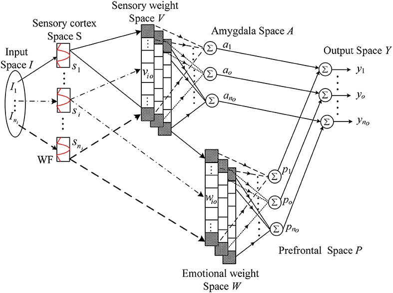
Figure 1. Structure of WFBELC.
Structure of WFBELC
The emotional system and sensory system receive inputs from sensory cortex. Both of them have 5 layers. The signal transmission and the main function of these layers are presented as follows.
1) Layer 1
The layer 1 is the input space I. For a given, ∈ ℜni Ii is an input state variable equaling to an actual input signal.
2) Layer 2
The layer 2 is the sensory cortex space S which performs the fuzzification operation of WFBELC. In this space, wavelet functions are adopted as the basis function with the uniformly distributed translations and the same dilations in order to describe the linguistic terms.
It has been proved that the integration of a Gaussian function is bounded and convergent. Therefore, all the derivatives of Gaussian function satisfy the admissibility condition of wavelet, and the n-order derivative of Gaussian function has the n-order vanishing moment. Thus, it is beneficial to compress data and eliminate noise, and possesses the better time-frequency localization properties (Zhao and Lin, in press). Therefore, in this paper, a type-1 Gaussian membership function is used as the mother wavelet. This Gaussian-type mother wavelet function can be expressed as:
Where si is the input from sensory cortex, which is the intensity of the individual stimulus components, Fi = (Ii – αi)/βi, where αi and βi are the i-th translation and the i-th dilation for the Gaussian-type wavelet of the i-th input Ii, respectively.
Because of the use of wavelet functions, the approximation ability for complex nonlinear functions is more effective than other basis functions, like the triangle basis function, the Gaussian basis function. Therefore, the learning speed is also increased.
3) Layer 3
The layer 3 is the weight space W. In this space, each block is a fuzzy output, which indicates the inference part of the fuzzy rules.
For the amygdala system, this space is known as the sensory weight space V, expressed in a vector form:
For the prefrontal system, this space is known as the emotional weight space W, expressed in a vector form:
where vio and wio represent the o-th weight value of the i-th input for the prefrontal system and the amygdala system, respectively.
4) Layer 4
The layer 4 is the weighted sum of the sensory input si, which can be solved by the method of center of gravity defuzzification.
For the amygdala system, the defuzzification operator is defined as:
For the prefrontal system, the defuzzification operator is defined as:
where φ is in a vector form, and φi is the constant values of the i-th fuzzy rule. They can be defined as
when , (6 and 7) can be redefined as:
5) Layer 5
The layer 5 is the output of the WFBELC. It is the result of interaction between the amygdala system and the prefrontal system. Thus, the o-th output of WFBELC is obtained as the following:
Updating Algorithm and Convergence Analysis of WFBELC
Updating Algorithm for the Brain Emotional Learning Controller
The emotional learning of the brain is achieved by updating the weights vio and wio. According to the neurophysiological prototype, the main function of the amygdala is to predict and respond to specific emotional hints. By adjusting the orbital frontal cortex, the difference between amygdala output and emotional implication tends to minimized (Lucas et al., 2004). Therefore, in view of the emotional learning approach of the brain, the parameters adaptation laws of the amygdala system and prefrontal system are respectively applied as
where ηv is a learning-rate in the amygdale cortex and ηw is a learning rate in the prefrontal cortex.
The parameter θo is an adjustment denoting the emotional signal or reinforcing signal for the o-th output of WFBELC, which is a function of several parameters. In this paper, θo is represented as
where λi and γo are the signal constant gains.
In order to represent the capability of forgetting the previous emotion signals, a maximum term is also added to Equation (13) as suggested in Fatourechi et al. (2001). Thus, the weight of amygdala cannot be decreased because the max function adjusts the weight monotonically. However, the prefrontal's learning rule is essentially different from the amygdala's. The orbitofrontal connection weight, seen from Equation (14), can resize the value to achieve the required output.
The updating laws for the weights of the amygdala system and the prefrontal system are written as:
Gradient Descent Algorithm for the Sensory Cortex Space
To update the translation parameter mi and the dilation parameter σi for a wavelet function, which are used in the sensory cortex space S, the normalized iterative gradient decent algorithm is applied. The back propagation is designed to deduce the parameter adaptation laws.
Firstly, an energy function E is defined as
where eo(k) = To(k) –yo(k) denotes the o-th error, To(k) is the o-th target output, yo(k) is the o-th output of WFBELC.
Thus, the parameter updating learning law can be derived according to
where ηα is the learning rate of translation, ηβ is the learning rate of dilation, and α = [α1, α2, …, αi, …, αni]T, β = [β1, β2, …, βi, …, βni]T
The gradient operation factors and are defined as
Then, by using the chain rule, the updating regulations of these two parameters can be expressed
Convergence Analysis
The following form is used to describe a class of uncertain nonlinear systems:
where x(t), u(t), d(t) and ys are the system state, the control signal, the external disturbance and the system output, respectively. The x(t) and u(t) can be defined as and , belonging to . The term x(t) is thought to be obtainable, defined as . Moreover, f(x(t)) is the system nonlinear vector, expressed as f0(x(t)) + Δf(x(t)) and G(x(t)) is the matrix-valued function, expressed as G0(x(t)) + ΔG(x(t)). Here, the second parts of them are the uncertain functions of the system whose boundaries are assumed to be obtainable, and the inverse of G0(x(t)) exists. Consequently, the unknown uncertainty of the system is described by these unknown items in Equation (25), i.e.Δf(x(t)), ΔG(x(t))u(t), and d(t), represented as L(x(t)) ∈ ℜno. Its boundary is also thought to be obtainable.
Here, we define a tracking error as e(t) = yd(t) − ys(t), its vector form is
A sliding hyper-plane is used to express the integrated error function
where , i = 1, 2, …, ni, are matrices with positive constant and define K = [K1T, …, KnT]T , is a sliding surface vector.
When the uncertainty and the nominal functions, such as L(x(t)), f0(x(t)) and G0(x(t)), are really known, we can design an ideal controller as
A dynamic equation of the tracking error can be given after replacing (Equation 25) with the ideal controller shown in Equation (28)
By selecting the value of K in Equation (29), the roots of the polynomial can locate in the left half of the complex plane. It means that with the time goes by, the tracking error will become smaller and smaller until it converges to zero. In practice, however, this uncertainty L(x(t)) is usually not obtained, so the ideal controller u*(t) in Equation (28) can not be implemented.
Therefore, a WFBELC controller and a robust controller are needed to be combined into a WFBELC control system to deal with this problem.
Thus, in this proposed WFBELC control system, there are a main controller uWFBELC and a robust compensator controller ur. The uWFBELC is utilized to approach the ideal controller u*(t), while the function of the compensator controller is to compensate the approximation error ε between u*(t) and uWFBELC.
Then, a LWFBELC would be appeared to approximate the L(x(t)) according to the universal approximation theorem (Wang, 1994).
Take the derivative of Equation (27) and use (Equation 25), then
Substituting (Equation 30) into (Equation 32), multiplying each side by sT gives
where
In the course of observation, the approximation error ε in Equation (31) is assumed to be bounded and the boundary is difficult to obtain. Therefore, we define an estimated value to estimate the boundary of this error.
where N is the boundary, whose estimated value is . Then, it can be assumed to bound ε ∈ [0, N].
Hence, the compensator in Equation (30) can be selected as
And (Equation 32) is also rewritten as
In this paper, a Lyapunov function is given as
where ηN is the learning rate of Ñ, whose adaptive learning law is selected as
Because of the constant value, .
Taking the derivative of Equation (38), and using (Equations 36, 37), then
Substituting (Equations 35, 40) into (Equation 38), becomes
Since is negative semidefinite function, i.e., , it indicates s and Ñ are bounded.
Let function Ξ = (N − |ε|)s, and integrate Ξ(t), obtains
Because Γ(s(0), Ñ(0)) is bounded, and Γ(s(t), Ñ(t)) is non-increasing and bounded, we derive:
In addition, according to Barbalat's lemma (Slotine and Li, 1991), since possesses the boundary, Ξ(t) → 0 when t → ∞. Hence, the WFBELC system possesses the asymptotic stability and satisfactory convergence. The tracking error will approximate to zero in virtue of t → ∞. A favorable robust tracking performance can be achieved consequently.
Moreover, the actual system and mathematical model are not exactly matched. To solve this problem, the uncertainty of these mathematical functions can be used to include these mis-matches. As a result, this WFBELC control system can be used for nonlinear systems with uncertainties to enhance their robust control characteristics.
Simulation Results
Two chaotic systems are used as the cases to verify the effectiveness of the presented WFBELC mode applied for uncertain nonlinear systems. For comparison, some other models are also applied.
Duffing-Holmes Chaotic System
Chaotic system is a kind of uncertain nonlinear systems, which is complex and unpredictable. Its disorder randomness is derived from the nonlinear term in the internal dynamics equation. One of the characteristics of chaotic systems is their high sensitivity to initial conditions, such that even very tiny differences in initial conditions may have a great impact on the behavior of these systems (Chang and Yan, 2005). The Duffing-Holmes chaotic system is considered. It is a second-order chaotic system expressed as Yan et al. (2005):
where p1 is the damping coefficient, qcos(ωt) is the periodic driving signal and q is the amplitude.
For different q values, the trajectories of the chaotic system are different, just as seen in Figures 2A–C with the real constants [p1, p2, p3] = [−1, 1, 0.25]. When q = 0.1, the trajectory is centered around a point (1, 0). When q = 1, the chaotic phenomenon appears, and the trajectory is periodically run around two points, (−1, 0) and (1, 0). When q = 8, besides the above characteristics, the trajectory is sunken toward the interior of orbit and cross state is emerged.
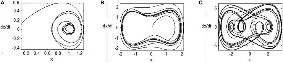
Figure 2. Phase plane of uncontrolled chaotic system (A) q = 0.1, (B) q = 1, and (C) q = 8.
When we take into account the unknown factors, the external interference signals, and the system control signals, a dynamic Equation (46) is given:
where the uncertainty term Δf(X, t) and the disturbance d(t) are selected as and 0.1 × sin(t).
Then, an adaptive WFBELC control for uncertain chaotic system is built in Figure 3.
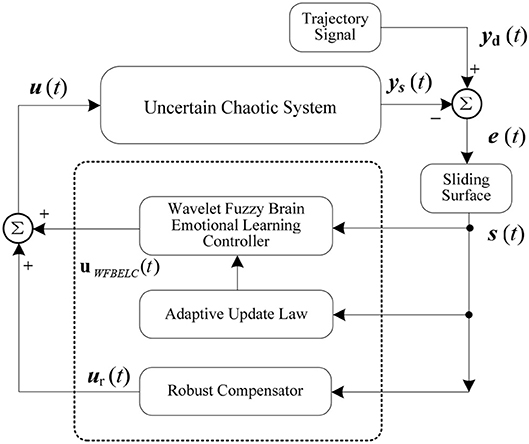
Figure 3. Adaptive WFBELC control for uncertain chaotic system.
For the example, the initial values of a sliding hyper-plane are selected as , k11 = 0.6, k12 = 0.02, which are based on the stable integrated error function in Equation (27). The dilation parameter for a wavelet function is set as βi = 3, and the translation parameter for a wavelet function is distributed in the interval [-2, 2].
Choosing an appropriate learning rate for the parameter updating law is one of the most important aspects of network design. Here, the learning rates in the amygdala and in the prefrontal cortex, ηv and ηw, are both equal to 0.01 according to Zhao and Lin (2017). The constant gains in Equation (15) are selected as λi = 60, (i = 1, 2), γo = 1.2, (o = 1). The compensator parameter ηN = 0.1, . These parameters are selected based on some trial-error method to ensure the required transient performance of this control system. Other parameters are random.
For the sake of verifying the effectiveness of WFBELC, an FCMAC (El-Sousy and Abuhasel, 2016) and a BELC (Chung and Lin, 2014) are also applied with different q value in Equation (46). A performance index P is defined as . The trajectory signal is set as yd(t) = x1(t) = sin(1.1 t). Simulation results with q = 0.3 of FCMAC, BELC and WFBELC are respectively depicted in Figures 4–8, namely: the periodic orbit phase plane plots, the response tracking curves of state x1 and state x2, the change trend chart of the control signal u and performance Index P. For the case of q = 8, there are also the set of such diagrams depicted in Figures 9–13. The values of root mean square error (RMSE) and the computation cost of this chaotic system using different models are listed in Table 1.
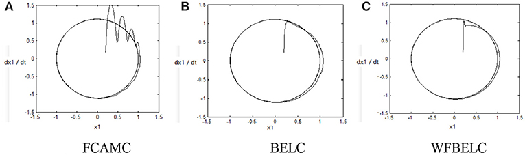
Figure 4. Periodic orbit phase plane plots (q = 0.3) (A) FCAMC, (B) BELC, and (C) WFBELC.
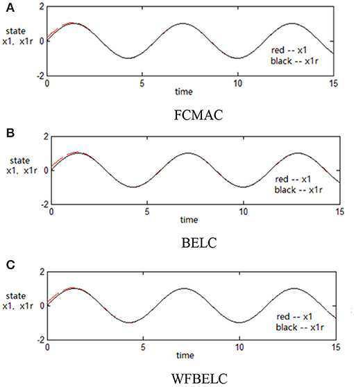
Figure 5. Response tracking curves of state x1 (q = 0.3) (A) FCMAC, (B) BELC, and (C) WFBELC.
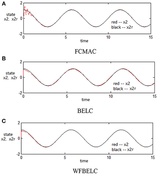
Figure 6. Response tracking curves of state x2 (q = 0.3) (A) FCMAC, (B) BELC, and (C) WFBELC.
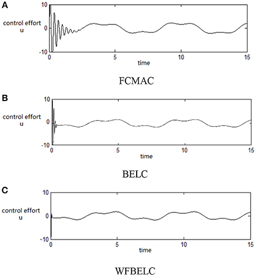
Figure 7. Change trend chart of the control signal u (q = 0.3) (A) FCMAC, (B) BELC, and (C) WFBELC.
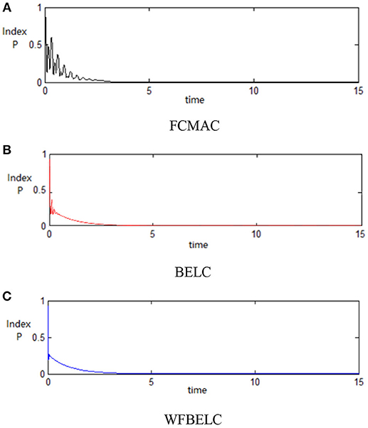
Figure 8. Performance Index P (q = 0.3) (A) FCMAC, (B) BELC, and (C) WFBELC.
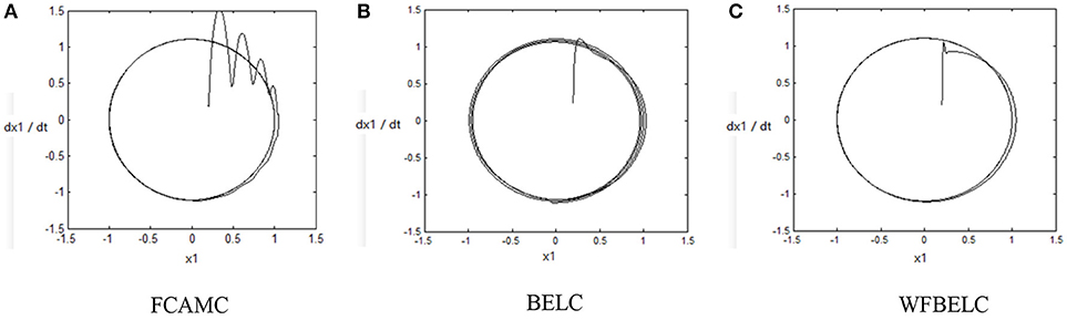
Figure 9. Periodic orbit phase plane plots (q = 8) (A) FCAMC (B) BELC (C) WFBELC.
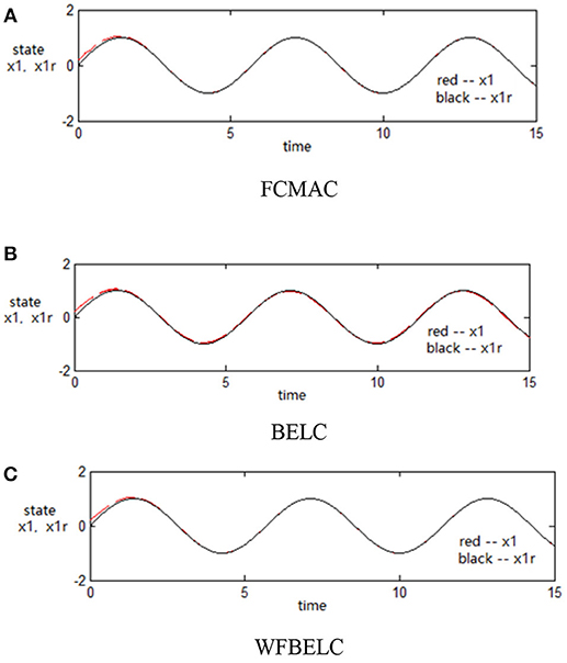
Figure 10. Response tracking curves of state x1 (q = 8) (A) FCMAC, (B) BELC, and (C) WFBELC.

Figure 11. Response tracking curves of state x2 (q = 8) (A) FCMAC, (B) BELC, and (C) WFBELC.
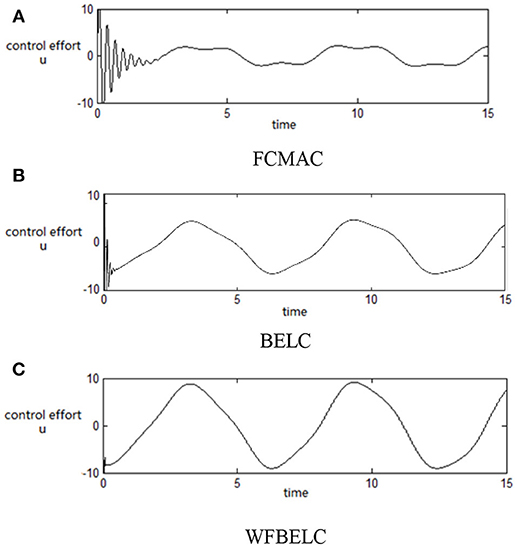
Figure 12. Change trend chart of the control signal u (q = 8) (A) FCMAC, (B) BELC, and (C) WFBELC.
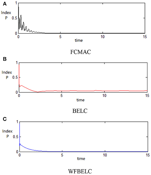
Figure 13. Performance Index P (q = 8) (A) FCMAC, (B) BELC, and (C) WFBELC.
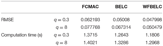
Table 1. Results for Duffing-Holmes chaotic system.
According to the above compared results, for different chaotic trajectories, much more satisfactory control performance can be obtained by using the presented WFBELC than by using the FCMAC or by using the BELC. The more serious the chaos is, the better the tracking performances of the WFBELC are. The control system with WFBELC model structure has smaller tracking error than the control system with other two model structures. Moreover, the convergence speed of the WFBELC model is also the fastest compared with the other two models. From Table 1, it can be seen that there are more parameters to upgrade the effectiveness of WFBELC control system than those of the other two control systems, so it costs a little more time in computation. This increased computation time is still acceptable.
Chua's Chaotic Circuit
A typical kind of the Chua's chaotic circuit structure is shown in Figure 14.
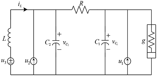
Figure 14. Chua's chaotic circuit.
Then the dynamic equations for this circuit are given as Chang and Robust (2004).
where R, g, C1, C2, and L are the physical parameters, i.e., the linear resistor, the nonlinear resistor, the capacitor and the inductor. The expresses the disturbance signal and expresses the control signal. The vC1(t), vC2(t) and the iL(t) are the state variables of the voltages and the current for this chaotic circuit. Thus, the input state vector of this circuit can be given as . These aforementioned dynamic equations are re-given as
and
The external disturbance is given as
The parameters of the resistance, inductance, and capacitance are formed as R = R0+ΔR, g(vC1) = g0(vC1)+Δg(vC1),L = L0 +ΔL,C1 = C10+ΔC1,C2 = C20+ΔC2, where R0, g0(vC1), L0, C10, and C20 are the nominal values and ΔR, Δg(vC1), ΔL, ΔC1, and ΔC2 represent the unknown nonlinear time-varying perturbations. The nominal values are set as R0 = 5, , L0 = 1, C10 = 1, and C20 = 0.5. The time-varying perturbations are ΔR = sin(0.5t), Δg(vC1) = 0.2 vC1×sin(t), ΔL = 0.15, ΔC1 = 0.1cos(0.5 t) +0.1 and ΔC2 = 0.1. The required trajectories are xr = [xr1, xr2, xr3] T = [1/5 × sin(3t)+sin(t), 1/5 × cos(3t)+cos(t), sin(t)+1] T (Joe et al., 2014). The initial values of state parameters, like the system states and the reference model states, are set as x1(0) = 0, x2(0) = −1, x3(0) = 0; xr1(t) = 0, xr2(t) = 1, xr3(t) = −1. A sliding hyper plane, s(e, t) = e(t), is proposed as for the proposed control case.
For the proposed WFBELC control system, the input signals of WFBELC are e1(t), e2(t), and e3(t), the initial parameters of sliding mode are set as K1 = diag(0.1, 0.1, 0.1) based on Equation (27). The dilation parameter for a wavelet function is set as βi = 1.6 and the translation parameter for a wavelet function is distributed in the interval [−2, 2].The learning rates in the sensory cortex space are selected as ηv = ηw = 0.15. The other parameters are set as same as in Example 1.
For comparison, a FCMAC and a BELC are also applied. The simulation results of this chaotic example are plotted as follows: the trajectory responses [vC1(t), vC2(t), iL(t)] are plotted in Figure 15; the enlarged responses are plotted in Figure 16, the dotted lines represent the reference signals and the red lines represent the responses; the corresponding control inputs [u1(t), u2(t), u3 (t)] are plotted in Figure 17; and the values of tracking error [e1(t), e2(t), e3 (t)] are plotted in Figure 18. The RMSE and the computation cost of these systems are tabulated in Table 2.
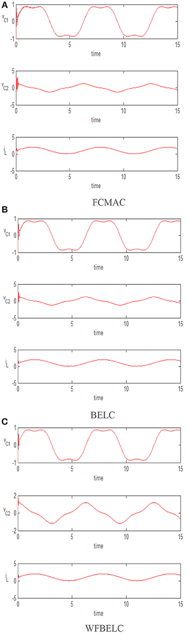
Figure 15. Trajectory responses (A) FCMAC, (B) BELC, and (C) WFBELC.
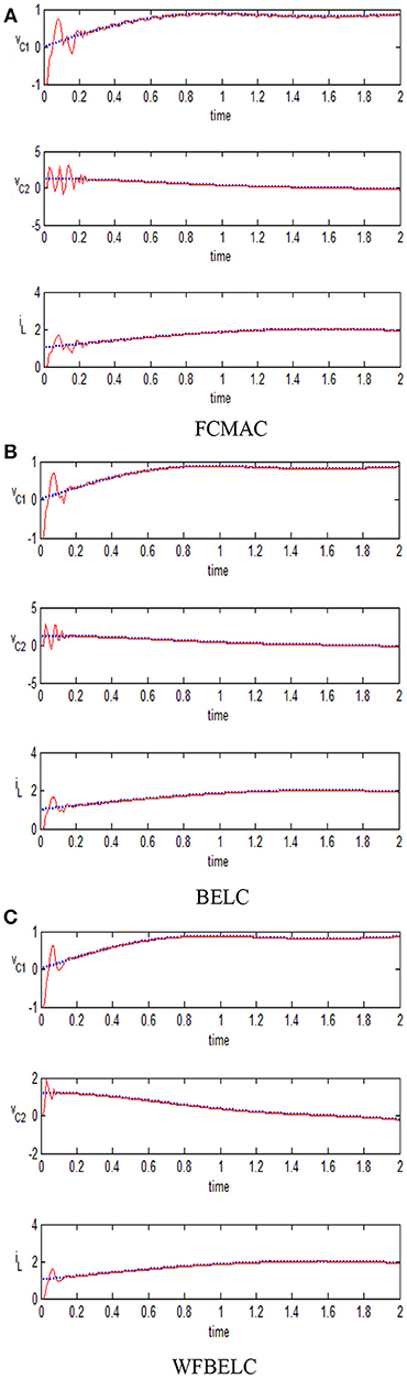
Figure 16. Enlarged responses (A) FCMAC, (B) BELC, and (C) WFBELC.
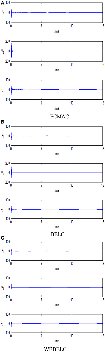
Figure 17. Corresponding control inputs (A) FCMAC, (B) BELC, and (C) WFBELC.
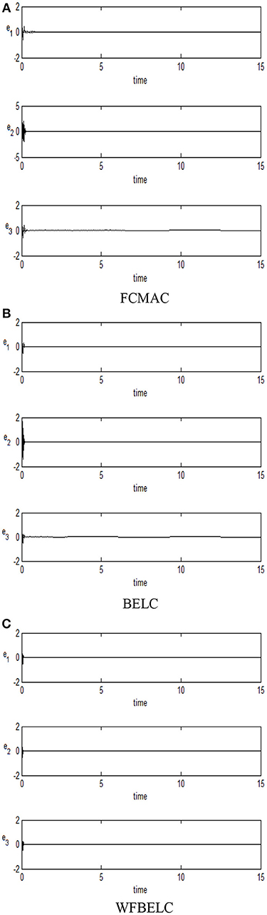
Figure 18. Values of tracking error (A) FCMAC, (B) BELC, and (C) WFBELC.
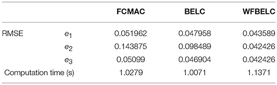
Table 2. Results for Chua's chaotic circuit.
In these simulations, from the Figures 15–18 and Table 2, the WFBELC control system can achieve faster errors convergence and reduce tracking error to get smaller tracking errors than the FCMAC control system and the traditional BELC control system. The tracking error convergence speed of the WFBELC is also faster than that of these two other systems. Moreover, it obtains obviously from Table 2 that for the same chaotic circuit, the RMSE of the WFBELC control system is smaller than the other two control systems. Similar to the previous example, compared with other models, the computation time has increased slightly by using the WFBELC model to improve the effectiveness of WFBELC control system. It is acceptable, as well.
Conclusions
The main contribution of this paper is to design the WFBELC model, which can be applied to much more effectively solve the uncertainty of the MIMO nonlinear systems. It consists of the wavelet theory, the type −1 fuzzy inference and the BEL algorithm. Thus, the WFBELC model has the advantages of them such that it can mimic the expression of the brain's sensations and emotions in one, and can describe the complex uncertain nonstationary signals more detailed. When the WFBELC is used as the main tracking controller for a MIMO uncertain nonlinear system and the robust compensation controller is used as a compensator, the control performances can be improved. Simulation results of two chaotic systems confirm that this proposed WFBELC model can effectively obtain satisfactory control capability with better transient responses and smaller error values comparing to the FCMAC control scheme and the BELC control scheme. Finally, the satisfactory control performance can be obtained much more quickly and effectively than other schemes. These comparisons also show that the proposed model can be more capable to handle the influence of the uncertainty. Moreover, the proposed control method can also be suitable for a large class of unknown nonlinear systems, because it does not need to know the accurate mathematical model of a nonlinear system. Applying the proposed model and the control scheme to real systems will be our future work. The favorable performance of the WFBELC can be further verified through the test results of the hardware platform.
Author Contributions
All authors listed have made a substantial, direct and intellectual contribution to the work, and approved it for publication.
Funding
This work was supported in part by the Research Project of High-level Talents (YKJ18004R) of Xiamen University of Technology, the Open Fund Research Project (201801)of the Fujian Key Lab of Medical Instrument and Pharmaceutical Technology, the Natural Science Foundation (2017J01509) of the Science and Technology Agency, Fujian, China, and Ministry of Science and Technology of Republic of China under grant MOST-103-2221-E-155-066-MY2.
Conflict of Interest Statement
The authors declare that the research was conducted in the absence of any commercial or financial relationships that could be construed as a potential conflict of interest.
Acknowledgments
We are grateful to the Editor-in-Chief, the Associate Editor, and reviewers for their constructive comments, so that the presentation of this paper has been greatly improved.
References
Abiyev, R. H., and Kaynak, O. (2008). Fuzzy wavelet neural networks for identification and control of dynamic plants—A novel structure and a comparative study. IEEE Trans. Ind. Electron. 55, 3133–3140. doi: 10.1109/TIE.2008.924018
Albus, J. S. (1975). A new approach to manipulator control: the cerebellar model articulation controller (CMAC). J. Dyn. Syst. Meas. Control 97, 220–227. doi: 10.1115/1.3426922
Balkenius, C., and MorÉn, Jan (2001). Emotional learning: a computational model of the amygdala. Cybern. Syst. 32, 611–636. doi: 10.1080/01969720118947
Chang, W. D., and Yan, J. J. (2005). Adaptive robust PID controller design based on a sliding mode for uncertain chaotic systems. Chaos Solitons Fractals 26, 167–175. doi: 10.1016/j.chaos.2004.12.013
Chang, Y. C., and Robust, H. (2004). control for a class of uncertain nonlinear time-varying systems and its application. IEE Proc. Control Theory Appl. 151, 601–609. doi: 10.1049/ip-cta:20040905
Chen, L., Liu, M., Huang, X., Fu, S., and Qiu, J. (2018). Adaptive fuzzy sliding mode control for network-based nonlinear systems with actuator failures. IEEE Trans. Fuzzy Syst. 26, 1311–1323. doi: 10.1109/TFUZZ.2017.2718968
Chung, C. C., and Lin, C. M. (2014). Brain emotional learning control system design for nonlinear systems. Int. J. Innovat. Res. Adv. Eng. 1, 70–74.
Chung, C. C., and Lin, C. M. (2015). Fuzzy brain emotional learning control system design for nonlinear systems. Int. J. Fuzzy Syst. 17, 117–128. doi: 10.1007/s40815-015-0020-9
Cui, R., Chen, L., Yang, C., and Chen, M. (2017). Extended state observer-based integral sliding mode control for an underwater robot with unknown disturbances and uncertain nonlinearities. IEEE Trans. Ind. Electron. 64, 6785–6795. doi: 10.1109/TIE.2017.2694410
Davanipoor, M., Zekri, M., and Sheikholeslam, F. (2012). Fuzzy wavelet neural network with an accelerated hybrid learning algorithm. IEEE Trans. Fuzzy Syst. 20, 463–470. doi: 10.1109/TFUZZ.2011.2175932
Dehkordi, B. M., Parsapoor, A., Moallem, M., and Lucas, C. (2011). Sensorless speed control of switched reluctance motor using brain emotional learning based intelligent controller. Energy Convers. Manag. 52, 85–96. doi: 10.1016/j.enconman.2010.06.046
El-Sousy, F. F. M., and Abuhasel, K. A. (2016). Self-organizing recurrent fuzzy wavelet neural network-based mixed H2/H∞ adaptive tracking control for uncertain two-axis motion control system. IEEE Trans. Ind. Applications 52, 5139–5155. doi: 10.1109/TIA.2016.2591901
Fatourechi, M., Lucas, C., and Khaki Sedigh, A. (2001). “Reduction of maximum overshoot by means of emotional learning,” Proceedings of 6th Annual CSI Computer Conference (Isfahan), 460–467.
Fu, S., Qiu, J., Chen, L., and Mou, S. (2018). Adaptive fuzzy observer design for a class of switched nonlinear systems with actuator and sensor faults. IEEE Trans. Fuzzy Syst. 26, 3730–3742. doi: 10.1109/TFUZZ.2018.2848253
Gosztolya, G., and Szilagyi, L. (2015). Application of fuzzy and possibilistic c-means clustering models in blind speaker clustering. Acta Polytechn. Hung. 12, 41–56. doi: 10.12700/aph.12.7.2015.7.3
Hsu, C. F., Su, C. T., and Lee, T. T. (2016). “Chaos synchronization using brain-emotional-learning-based fuzzy control,” in International Conference on Soft Computing and Intelligent Systems (Sapporo), 811–816.
Joe, H., Kim, M., and Yu, S.-C. (2014). Second-order sliding-mode controller for autonomous underwater vehicle in the presence of unknown disturbances. Nonlinear Dyn. 78, 183–196. doi: 10.1007/s11071-014-1431-0
Lahmiri, S., Boukadoum, M., and Chartier, S. (2013). A supervised classification system of financial data based on wavelet packet and neural networks. Int. J. Strateg. Decis. Sci. 4, 72–84. doi: 10.4018/ijsds.2013100105
Le Doux, J. E. (1992). The Amygdala: Neurobiological Aspects of Emotion. New York, NY: Wiley-Liss, 339–351.
Lin, C. M., Hou, Y. L., Chen, T. Y., and Chen, K. H. (2014). Breast nodules computer-aided diagnostic system design using fuzzy cerebellar model neural networks. IEEE Trans. Fuzzy Syst. 22, 693–699. doi: 10.1109/TFUZZ.2013.2269149
Lin, C. M., and Li, H. Y. (2014). Intelligent control using the wavelet fuzzy CMAC backstepping control system for two-axis linear piezoelectric ceramic motor drive systems. IEEE Trans. Fuzzy Syst. 22, 791–802. doi: 10.1109/TFUZZ.2013.2272648
Liu, Z., Chen, C. L. P., Zhang, Y., Li, H. X., and Wang, Y. (2013). A three-domain fuzzy wavelet system for simultaneous processing of time-frequency information and fuzziness. IEEE Trans. Fuzzy Syst. 21, 176–183. doi: 10.1109/TFUZZ.2012.2204265
Lu, C. H. (2011). Wavelet fuzzy neural networks for identification and predictive control of dynamic systems. IEEE Trans. Ind. Electron. 58, 3046–3058. doi: 10.1109/TIE.2010.2076415
Lucas, C., Shahmirzadi, D., and Sheikholeslami, N. (2004). Introducing BELBIC: brain emotional learning based intelligent controller. Intell. Autom. Soft Comput. 10, 11–21. doi: 10.1080/10798587.2004.10642862
Nikolić, M., Jovanović, D. P., Lim, Y. L., Bertling, K., Taimre, T., and Rakić, A. D. (2013). Approach to frequency estimation in self-mixing interferometry: multiple signal classification. Appl. Opt. 52, 3345. doi: 10.1364/AO.52.003345
Rolls, E. T. (1986). “A theory of emotion, and its application to understanding the neural basis of emotion,” in Emotions: Neural and Chemical Control, ed Y. Oomura (Tokyo: Japan Scientific Societies Press), 325–344.
Rolls, E. T. (1995). “A theory of emotion and consciousness, and its application to understanding the neural basis of emotion,” in The Cognitive Neurosciences, ed M. S. Gazzaniga (Cambridge, MA: MIT Press), 1091–1106.
Roshanaei, M., Vahedi, E., and Lucas, C. (2010). Adaptive antenna applications by brain emotional learning based on intelligent controller. IET Microwaves Antennas Propagat. 4, 2247–2255. doi: 10.1049/iet-map.2009.0101
Schultz, W., Romo, R., Ljungberg, T., Mirenowicz, J., Jollerman, J. R., and Dickinson, A. (1995). “Reward-related signals carried by dopamine neurons,” in Models of Information Processing in the Basal Ganglia (Cambridge, MA: MIT Press), 233–248.
Sharbafi, M. A., Lucas, C., and Daneshvar, R. (2010). Motion control of omni-directional three-wheel robots by brain-emotional-learning-based intelligent controller. IEEE Trans. Sys. Man Cybern. Part C 40, 630–638. doi: 10.1109/TSMCC.2010.2049104
Slotine, J. J. E., and Li, W. P. (1991). Applied Nonlinear Control, Englewood. Cliffs, NJ: Prentice-Hall.
Su, X., Liu, X., Shi, P., and Yang, R. (2017). Sliding mode control of discrete-time switched systems with repeated scalar nonlinearities. IEEE Trans. Autom. Control 62, 4604–4610. doi: 10.1109/TAC.2016.2626398
Thompson, R. F. (1998). The neural basis of basic associative learning of discrete behavioral responses. Trends Neurosci. 11, 152–155. doi: 10.1016/0166-2236(88)90141-5
Wang, L. X. (1994). Adaptive Fuzzy Systems and Control: Design and Stability Analysis, Englewood. Cliffs, NJ: Prentice-Hall.
Wen, S., Chen, M. Z., Zeng, Z., Huang, T., and Li, C. (2017). Adaptive neural-fuzzy sliding-mode fault-tolerant control for uncertain nonlinear systems. IEEE Trans. Syst. Man Cybern. Syst. 47, 2268–2278. doi: 10.1109/TSMC.2017.2648826
Yan, J. J., Shyu, K. K., and Lin, J. S. (2005). Adaptive variable structure control for uncertain chaotic systems containing dead-zone nonlinearity. Chaos Solitons Fractals 25, 347–355. doi: 10.1016/j.chaos.2004.11.013
Yeo, C. H., and Hesslow, G. (1998). Cerebellum and conditioned reflexes. Trends Cogn. Sci. 2, 322–331. doi: 10.1016/S1364-6613(98)01219-4
Yu, W., Wang, H., Cheng, F., Yu, X., and Wen, G. (2017). Second-order consensus in multiagent systems via distributed sliding mode control. IEEE Trans. Cybern. 47, 1872–1881. doi: 10.1109/TCYB.2016.2623901
Zarchi, H. A., Daryabeigi, E., Markadeh, G. R. A., and Soltani, J. (2011). “Emotional controller (BELBIC) based DTC for encoderless synchronous reluctance motor drives,” in 2011 2nd Power Electronics, Drive Systems and Technologies Conference (Tehran), 478–483.
Zhang, S., Wang, J., Wang, Z., Gong, Y., and Liu, Y. (2015). Multi-target tracking by learning local-to-global trajectory models. Pattern Recognit. 48, 580–590. doi: 10.1016/j.patcog.2014.08.013
Zhao, J., and Lin, C. M. (2017). An interval-valued fuzzy cerebellar model neural network based on intuitionistic fuzzy sets. Int. J. Fuzzy Syst. 19, 881–894. doi: 10.1007/s40815-017-0321-2
Zhao, J., and Lin, C. M (in press). Wavelet-TSK-type fuzzy cerebellar model neural network for uncertain nonlinear systems. IEEE Trans. Fuzzy Syst. doi: 10.1109/TFUZZ.2018.2863650
Zheng, E. H., Xiong, J. J., and Luo, J. L. (2014). Second order sliding mode control for a quadrotor UAV. ISA Trans. 53, 1350–1356. doi: 10.1016/j.isatra.2014.03.010
Zhong, Z., Zhu, Y., and Ahn, C. K. (2018b). Reachable set estimation for Takagi-Sugeno fuzzy systems against unknown output delays with application to tracking control of AUVs. ISA Trans. 78, 31–38. doi: 10.1016/j.isatra.2018.03.001
Zhong, Z. X., and Zhu, Y. Z. (2017). Observer-based output-feedback control of large-scale networked fuzzy systems with two-channel event-triggering. J. Franklin Inst. 354, 5398–5420. doi: 10.1016/j.jfranklin.2017.05.036
Zhong, Z. X., Zhu, Y. Z., and Lam, H. K. (2018a). Asynchronous piecewise output-feedback control for large-scale fuzzy systems via distributed event-triggering schemes. IEEE Trans. Fuzzy Syst. 26, 1688–1703. doi: 10.1109/TFUZZ.2017.2744599
Zhou, Q., Chao, F., and Lin, C. M. (2017). A functional-link-based fuzzy brain emotional learning network for breast tumor classification and chaotic system synchronization. Int. J. Fuzzy Syst. 20, 349. doi: 10.1007/s40815-017-0326-x
Keywords: wavelet function, brain emotional neural network, fuzzy system, uncertainty, compensator controller
Citation: Zhao J, Lin C-M and Chao F (2019) Wavelet Fuzzy Brain Emotional Learning Control System Design for MIMO Uncertain Nonlinear Systems. Front. Neurosci. 12:918. doi: 10.3389/fnins.2018.00918
Received: 30 July 2018; Accepted: 22 November 2018;
Published: 04 January 2019.
Edited by:
Yanzheng Zhu, Western Sydney University, AustraliaReviewed by:
Yu Chen, University of Maryland, United StatesLiheng Chen, Harbin Engineering University, China
Jinlong Ma, Hebei University of Science and Technology, China
Copyright © 2019 Zhao, Lin and Chao. This is an open-access article distributed under the terms of the Creative Commons Attribution License (CC BY). The use, distribution or reproduction in other forums is permitted, provided the original author(s) and the copyright owner(s) are credited and that the original publication in this journal is cited, in accordance with accepted academic practice. No use, distribution or reproduction is permitted which does not comply with these terms.
*Correspondence: Jing Zhao, enR1bGlwd29ya0AxMzkuY29t
Chih-Min Lin, Y21sQHNhdHVybi55enUuZWR1LnR3