 Zhengshi Yang1
 Xiaowei Zhuang1
 Christopher Bird1
 Karthik Sreenivasan1
 Virendra Mishra1
 Sarah Banks1
 Dietmar Cordes1,2* and the Alzheimer's Disease Neuroimaging Initiative†
- 1Cleveland Clinic Lou Ruvo Center for Brain Health, Las Vegas, NV, United States
- 2Departments of Psychology and Neuroscience, University of Colorado, Boulder, CO, United States
Collecting multiple modalities of neuroimaging data on the same subject is increasingly becoming the norm in clinical practice and research. Fusing multiple modalities to find related patterns is a challenge in neuroimaging analysis. Canonical correlation analysis (CCA) is commonly used as a symmetric data fusion technique to find related patterns among multiple modalities. In CCA-based data fusion, principal component analysis (PCA) is frequently applied as a preprocessing step to reduce data dimension followed by CCA on dimension-reduced data. PCA, however, does not differentiate between informative voxels from non-informative voxels in the dimension reduction step. Sparse PCA (sPCA) extends traditional PCA by adding sparse regularization that assigns zero weights to non-informative voxels. In this study, sPCA is incorporated into CCA-based fusion analysis and applied on neuroimaging data. A cross-validation method is developed and validated to optimize the parameters in sPCA. Different simulations are carried out to evaluate the improvement by introducing sparsity constraint to PCA. Four fusion methods including sPCA+CCA, PCA+CCA, parallel ICA and sparse CCA were applied on structural and functional magnetic resonance imaging data of mild cognitive impairment subjects and normal controls. Our results indicate that sPCA significantly can reduce the impact of non-informative voxels and lead to improved statistical power in uncovering disease-related patterns by a fusion analysis.
Introduction
Collecting multiple modalities of neuroimaging data on the same subject is increasingly becoming the norm in clinical practice and research. Neuroimaging multi-modality data were traditionally analyzed and interpreted separately to find disease-related or task-related patterns in the brain. However, analyzing each modality independently does not necessarily find related patterns in both modalities. A single pattern in one modality might be related with a mixture of patterns in another modality. Fusing multiple modalities to find related patterns is a challenge in neuroimaging analysis. In the last decade, several techniques were proposed to utilize multiple imaging modalities, including data integration (Savopol and Armenakis, 2002; Calhoun and Adal, 2009), asymmetric data fusion (Filippi et al., 2001; Kim et al., 2003; Henson et al., 2010) and symmetric data fusion techniques (Correa et al., 2008; Groves et al., 2011; Sui et al., 2011; Le Floch et al., 2012; Lin et al., 2014; Mohammadi-Nejad et al., 2017). A detailed review about these techniques can be found in Calhoun and Sui (2016). In the data integration technique, each dataset is analyzed independently, and, then, one dataset is overlaid on another without considering the interaction among datasets. Asymmetric data fusion utilizes one dataset to improve the analysis of another dataset. For example, Kim et al. (2003) used the foci of functional magnetic resonance imaging (fMRI) activation as seed points for Diffusion Tensor Imaging fiber reconstruction algorithms. Filippi et al. (2001) integrated conventional magnetic resonance imaging (MRI) and diffusion tensor MRI to better locate white matter lesions in multiple sclerosis subjects. Henson et al. (2010) constrained the electromagnetic sources of Magnetoencephalography and Electroencephalography (MEG, EEG) data with fMRI as empirical priors. Along with advantages of asymmetric data fusion techniques, asymmetric fusion omits the fact that each imaging modality has an essentially unique nature (Calhoun and Sui, 2016). In the symmetric data fusion method, multiple imaging modalities are analyzed conjointly to optimize the information contributed by each modality. Multiple imaging modalities are combined to extract complementary information regarding the integrity of the underlying neural structures and networks (Calhoun and Sui, 2016). In this study, we focus on symmetric data fusion using two modalities. Unless explicitly stated, data fusion refers to symmetric data fusion.
Canonical correlation analysis (CCA) is a multivariate method of finding linear combinations of two multidimensional random variables to maximize their correlation (Hotelling, 1936). CCA and its extensions have been extensively utilized in data fusion to associate related patterns across multiple data. A few CCA-based fusion methods were proposed in the last decade, such as multimodal CCA (Correa et al., 2008), source CCA + joint ICA (Sui et al., 2010) and multimodal CCA + joint ICA (Sui et al., 2011). The variant of CCA with more than two datasets, multiset CCA, was also applied in data fusion (Correa et al., 2010). When CCA is directly applied to the original data in a fusion analysis, some of the canonical variables are perfectly correlated regardless of the association among data, since the feature space is usually high-dimensional and only relatively few observations (subjects) are available (Pezeshki et al., 2004). In the CCA-based fusion methods mentioned above, principal component analysis (PCA) was used to reduce the data dimension. More specifically, a set of principal components with the largest possible variances are found by PCA and then the projections of original data (scores) on the space spanned by principal components are the dimension-reduced input data for the fusion CCA algorithm.
PCA solves the singularity problem in these fusion methods but does not take into account that in many cases only a small proportion of voxels (features), called informative voxels (features), have contribution to the variance, and a large proportion are non-informative. If principal components were obtained with non-informative voxels (features) assigned to zero, the projections of original data on the space spanned by the major principal components are more robust to non-informative voxels and thus helps CCA to better match related patterns across modalities. For example, when fusion analysis is applied to the data acquired from mild cognitive impairment (MCI) subjects and normal controls (NC), brain regions engaged in memory, language, and judgment (e.g., hippocampus, medial temporal lobe, frontal lobe) should be significant in the disease-related patterns (Forsberg et al., 2008; Bai et al., 2009). Specifying non-informative voxels to have zero weight could be beneficial for matching disease-related patterns by a fusion analysis. In general, properly suppressing non-informative voxels will further improve the statistical power of fusion techniques. Even though imaging data can be masked with predetermined regions of interest (ROIs) to address the feature selection process and avoid problems arising from non-informative voxels, ROI selection requires typically unavailable prior knowledge about the disease and patient cohort.
Selection and suppression of non-informative features in principal components can be automated by implementing sparsity in the PCA algorithm, called sparse PCA (sPCA) (Zou et al., 2006; Witten et al., 2009). The sPCA method and its extensions have been applied in multiple fields, such as machine learning, pattern recognition, and bioinformatics (Zou et al., 2006; Shen and Huang, 2008; Witten et al., 2009; Jenatton et al., 2010). A brief review of sPCA can be found in Feng et al. (2016). When comparing sPCA+CCA with PCA+CCA, sPCA produces different scores because of the reoriented space spanned by the principal components and, thus, sPCA influences the subsequent CCA step in associating multiple modalities.
Unlike sPCA+CCA having feature selection prior to fusing datasets, sparse CCA (sCCA) (Parkhomenko et al., 2009; Witten and Tibshirani, 2009; Lê Cao et al., 2011; Abdel-Rahman et al., 2014; Avants et al., 2014) has feature selection and data fusion applied at the same time. In this study, the sPCA+CCA method is compared with the sCCA method.
In the following, we first describe the theory behind sPCA and outline how to implement the sPCA algorithm. Then, we develop a cross-validation algorithm to optimally specify the sparsity parameter and the number of major principal components in sPCA. Then, we evaluate the improvement by introducing sparsity constraint to PCA using simulated data. Considering mild cognitive impairment (MCI) impacts both the function and structure in certain regions of the brain (Chetelat et al., 2002; Rombouts et al., 2005), we apply four fusion methods including sPCA+CCA, PCA+CCA [called multimodal CCA in Correa et al. (2008)], sCCA (Witten et al., 2009) and parallel ICA (Liu et al., 2009) on structural and functional MRI data of mild cognitive impairment (MCI) subjects and normal controls (NC), with the hypothesis to find disease-related association between these two modalities. Since disease-related features are visible in all modalities to varying degrees (Groves et al., 2011), fusion methods can match disease-related patterns in a two-group setting. Hence, the group discrimination and the correlation with β-amyloid measurement can be used to evaluate how well fusion methods match disease-related patterns across modalities.
Theory
Sparse Principal Component Analysis (sPCA)
Derivation of sPCA
Let X denote an n × m feature matrix with rank(X) ≤ min(n, m), where n is the number of observations and m is the number of features in each observation. If X is a brain map, as in our case, n is the number of subjects and m is the number of voxels. PCA transforms a set of observations of correlated variables into a set of uncorrelated orthogonal variables called principal components that can be ordered according to the magnitude of their eigenvalues. The first K principal components can be determined by minimizing the least square problem (Eckart and Young, 1936), expressed as
where M(K) is a set of matrices with rank(M) = K and means the squared Frobenius norm (see Appendix A in Supplementary Material for more detail). PCA is closely related to singular value decomposition (SVD). Using SVD, X can be decomposed into
where U ∈ ℝn×K and V ∈ ℝm×K are the left and right singular vectors of X satisfying the orthonormality condition, and D =diag(d1, …, dK) ∈ ℝK×Kis the diagonal matrix of ordered singular values of X with d1 ≥ d2 ≥ … ≥dK > 0. The optimal in M(K) can be written as
where and denote the i-th column vector of U and V, respectively. Following the notation in SVD, the objective function fobj for only one component can be written as
Considering that there are many voxels but few subjects, namely, m ≫ n, the sparsity in our study is only implemented to set non-informative voxels to be zero. Because V is a set of voxel-wise spatial maps, sparsity was incorporated into the projection vector vi but not the score vector ui, which is different than the sPCA method in Witten et al. (2009), who applied sparsity constraint on both singular vectors u and v. For this reason, we derived the sPCA formula with an L1 penalty on variable v added to the fobj(d, u, v) in Equation (4):
where the parameter c is the sparsity tuning parameter. A smaller c means that more elements in the principal component v are set to zero and the principal component becomes sparser. We would like to emphasize that sPCA has the elastic penalty consisting of the L1 and L2 penalty as shown in Appendix B in Supplementary Material, and, thus, the principal components from sPCA are well-defined and unique even when m ≫ n (Zou et al., 2006). Following the derivation in Appendix A in Supplementary Material, Equation (5) can be rewritten as:
As shown by Witten et al. (2009), if u or v is fixed, the criterion in Equation (6) is a convex problem in v or u.Thus, Equation (6) represents a biconvex problem. Because a convex problem can be solved reliably and efficiently, we solve Equation (6) by converting the equation into two convex sub-problems with u and v alternatingly fixed.
Iterative Algorithm for sPCA
Equation (6) is solved by an iterative algorithm modified based on the sPCA algorithm in Witten et al. (2009). We start with an initial value and then update v to maximize uTXv as expressed below
Appendix C in Supplementary Material shows that the optimal solution in Equation (7) is . The function S is the (vector-valued) soft threshold function given by S(a, μ) = sign(a)max(0, |a|−μ), where the sign (.) and |.| operation act on each element of vector a. If μ = 0 satisfies ||v||1 ≤ c, then . Otherwise, μ is determined efficiently by a binary search algorithm to have ||v||1 = c. At a fixed v, Equation (6) becomes
The optimal u is simply the unit vector along direction b, namely, . The alternating iteration stops when a convergence criterion is satisfied. Then X is updated by removing the variance contained in the previous principal component by X←X−duvT, and the next pair of u and v is computed by the same iterative algorithm until K principal components are found.
Parameters Selection in sPCA by Split-Sample Cross Validation
A ten-fold cross validation method is used to estimate the parameters in sPCA, including the optimal sparsity tuning parameter c* and the best number of principal components K*. The flow chart for the split-sample cross validation method is shown in Figure 1. For data matrix X, each subject is randomly assigned to one fold. Let X(f) denote the data from the subjects assigned in the f-fold dataset and denote the data except the data in the f-fold dataset. Principal components are computed from matrix , and then these principal components are applied on X(f) to estimate parameters based on a selection criterion, and, finally, the mean value of the estimated parameters in each fold of the data is used for fusion analysis. Mathematically, K-factor sPCA is applied on matrix by where and . Then, the principal components are used as regressors in a linear regression model to fit each sample in the untouched data X(f), namely, and . The Akaike Information Criterion (AIC) (Akaike, 1974; Shumway et al., 2000) is used to evaluate how close the reconstructed matrix is to X(f). The AIC provides a tradeoff between goodness-of-fit (minimum log-likelihood) and complexity of the model (Sui et al., 2010). Witten et al. (2009) used the mean-square-error (MSE) as the criterion in a cross-validation method that is based on an imputation algorithm (Troyanskaya et al., 2001). The optimal sparsity tuning parameter c* was selected by minimizing MSE with only the first principal component (K = 1) considered. This method cannot estimate the number of principal components K* since MSE always decreases with increasing K. We have revised the cross-validation method in Witten et al. (2009) with AIC as the criterion and compared AIC with the split-sample cross-validation method. We found that the split-sample method is more reliable and accurate in estimating parameters. Appendix D in Supplementary Material describes the calculation of AIC and the comparison of these two cross-validation methods in more detail. Let {c(f), K(f)} denote the parameters having minimum AIC for the f-fold cross-validation, the optimal sparsity tuning parameter c* is defined as the average over c(f), and the optimal number of principal components K* is the rounded integer of the average over K(f). The estimated parameter set {c*, K*} is used in the sPCA+CCA fusion analysis.
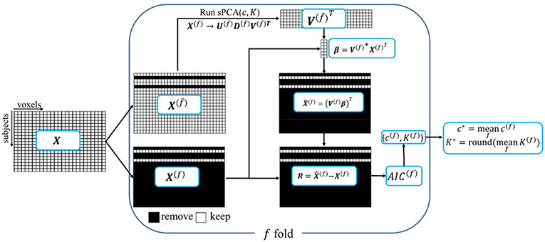
Figure 1. A schematic diagram of the split-sample cross-validation method in sPCA. X is the data matrix. Each subject is randomly assigned to one fold, X(f) denotes the data from the subjects assigned in f-fold data and X(f) denotes the data with X(f) excluded. The “+” superscript indicates the Moore-Penrose pseudoinverse.
sPCA+CCA
In sPCA+CCA, PCA is replaced by sPCA for dimension-reduction. The sPCA method is applied to reduce the data dimension for each modality separately, i.e., . In this step, the sparsity tuning parameter , r = 1,2, and the number of principal components , r = 1,2, are optimized for each modality by using the split-sample cross-validation method described in section Parameters Selection in sPCA by Split-Sample Cross Validation. The dimension-reduced dataset is the principal component score given by
Then, CCA is applied to link the data Y1 and Y2 by maximizing the canonical correlation between Y1Z1 and Y2Z2, where Zr, r = 1, 2, denote the canonical transformation matrices. The resulting canonical variates Ar = YrZr are called modulation profiles. Only the matched modulation profiles between datasets are correlated, and all other modulation profiles are uncorrelated, i.e.,
where ρd is the canonical correlation between A1d and A2d. Finally, the spatial maps C1 and C2 corresponding to A1 and A2, respectively, are calculated by least square estimation according to
where the “+” superscript indicates the Moore-Penrose pseudoinverse. In Equations (9) and (11) we could have used the original data matrix Xr instead of . A schematic flowchart of sPCA+CCA is shown in Figure 2.
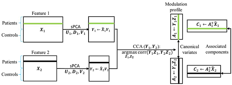
Figure 2. Flow chart of sPCA+CCA. sPCA was carried out reduce data dimensions and to suppress irrelevant features. Then, CCA was carried out for fusion analysis to obtain modulation profiles and associated components. In the flow chart , is the data matrix of the two modalities obtained from sPCA.
Materials and Methods
Simulation 1: sPCA vs. PCA
The simulation was carried out to evaluate whether sPCA is sensitive to the noise in the data at different sparsity levels. The simulated data X was generated based on the form X = YVT, where Y = […,yn, …] is the intrinsic principal component scores and V = […,vn, …] is a set of orthogonal maps. The simulation consists of 80 samples and 3 intrinsic principal components, hence Y has a dimension of 80 ×3. To analyze whether the improvement made by introducing sparsity to PCA relates to the spatial sparsity level of the signal, we have simulated the data with sparsity levels of 30, 50, and 70%. Here, the sparsity level is defined as the percentage of zero elements in the map. Figure 3 shows the principal component scores Y in Figure 3A and their corresponding spatial maps V at 70% sparsity level in Figure 3B without threshold. The images have a dimension of 91 ×109 ×3, and only the second slice of the spatial maps is shown.
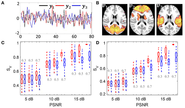
Figure 3. Simulation 1: Comparison of sPCA and PCA. (A) Simulated principal component scores Y = [y1, y2, y3]. (B) The spatial maps V = [v1, v2, v3] corresponding to the scores with 70% voxels having zero values. Simulated data were generated 100 times with PSNR as 5 dB, 10 dB and 15 dB and sparsity level as 0.3, 0.5, and 0.7. (C) Boxplot for the similarity value with true principal component scores SY. (D) Boxplot for the similarity value with true spatial maps SV. The boxplot for sPCA is shown in red and for PCA in blue.
Gaussian noise N was added to create noisy images and Gaussian smoothing with Full-Width-At-Half-Maximum (FWHM) of 8 mm was applied to introduce spatial correlation. The simulated data were generated with Peak Signal-to-Noise Ratio (PSNR) of 5, 10, and 15 dB, which are similar to the PSNRs used in Sui et al. (2010). PSNR is defined as
Here, maxval is the maximum possible pixel value and MSE is the mean squared error between noisy and noise-free images. A higher PSNR indicates a higher image quality. The simulation was carried out 100 times using the same Y and V, but with different noise realizations.
Simulation 2: Comparison of Fusion Methods
The simulation was carried out with sparsity level 70% at moderate signal-to-noise ratio with PSNR = 10 dB. The sparsity level used in the simulation is close to the estimated sparsity level in the real data as mentioned below in Parameter Selection section. Two simulated modalities were generated by following the steps described in section Simulation 1: sPCA vs. PCA except we replace the intrinsic principal component scores by modulation profile A1 and A2, respectively, for the first and second modality. The modulation profiles {A1, A2} satisfy the orthogonality condition in Equation (10). The canonical correlations ρ between A1 (red curve) and A2 (black curve) are [0.70, 0.45, 0.22] as shown in Figure 4A. The three corresponding pairs of sparse spatial maps are shown in Figure 4B. The first pair of canonical variables in {A1, A2} were simulated to be group-distinct using 40 subjects for each group. The simulation was carried out fifty times using the same modulation profiles and spatial maps, but with different noise realizations. The average performance is reported in the Result section.
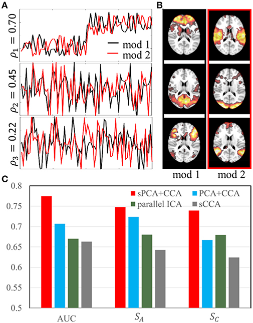
Figure 4. Simulation 2: Comparison of fusion methods. (A). Three pairs of simulated modulation profiles satisfying the orthogonality condition. (B). Simulated spatial maps at sparsity level 70%. (C) Bar plot of the AUC measurement, similarities (SA) between estimated and true modulation profiles, and their corresponding spatial maps (SC).
MRI/fMRI Data and PET Analysis
Structural MRI and resting-state fMRI data used in this study were downloaded from the publicly available ADNI database. The ADNI was launched in 2003 as a public-private partnership, led by Principal Investigator Michael W. Weiner, MD. The primary goal of ADNI has been to test whether serial MRI, positron emission tomography (PET), other biological markers, and clinical and neuropsychological assessment can be combined to measure the progression of mild cognitive impairment (MCI) and early Alzheimer's disease (AD).
The resting-state fMRI data, T1 structural data, and corresponding clinical data were downloaded from the ADNI 2 database before September 18, 2016. All subjects used in this study had florbetapir (18F) PET scans within 6 months of MRI scans. All MCI subjects had an absence of dementia (clinical dementia rating of 0.5), a memory complaint and objective memory loss measured by education adjusted scores on the Wechsler Logical Memory Scale II, an absence of significant levels of impairment in other cognitive domains and essentially had preserved activities of daily living. All subjects were scanned on a 3.0-Tesla Philips MRI scanner. The magnetization prepared rapid acquisition gradient echo (MP-RAGE) sequence was used to acquire T1-weighted structural images by the investigators of the ADNI consortium. The structural MRI scans were collected with a 24 cm field of view and a resolution of 256 ×256 ×170, to yield a voxel size of 1 ×1 ×1.2 mm. Resting-state fMRI data were acquired from an echo-planar imaging sequence with parameters: 140 time points; TR/TE = 3000/30 ms; flip angle = 80 degrees; 48 slices; spatial resolution = 3.3 mm ×3.3 mm ×3.3 mm and imaging matrix = 64 ×64. Details of the ADNI MRI protocol can be found on ADNI website (http://adni.loni.usc.edu/). If one subject had multiple MRI/fMRI scans satisfying the requirements specified above, the first available MRI/fMRI data set was used for analysis. The Standard Uptake Value Ratio (SUVR) analysis was carried out to measure ß-amyloid on ADNI florbetapir PET scans by site investigators and the SUVR data using a composite reference regions were downloaded from the ADNI website. The correlation between SUVR measurement and the result of fusion methods was used to evaluate the performance of different fusion methods. In total, 37 MCI subjects (age = 73.7 ± 6.7 years; gender = 19 female/18 male) and 42 NC subjects (age = 75.0 ± 7.3 years; gender = 24 female/18 male) were selected.
FMRI Data
Preprocessing
The first 5 volumes were excluded from the analysis. The fMRI time series were slice-timing corrected and realigned to the first volume using SPM12, co-registered to the individual T1 images and then normalized to the MNI152 2 mm template using Advanced Normalization Tools (ANTs) (http://stnava.github.io/ANTs/). Nuisance regression was carried out with six head motion parameters along with signals extracted from white matter and CSF [3-mm radius spheres centered at MNI coordinates (26, −12, 35) and (19, −33, 18)] (Chen et al., 2015). The resulting time series were smoothed further with a 10-mm Gaussian kernel and band-pass filtered to be in the frequency range 0.01–0.1 Hz. These steps were computed with MATLAB (The Mathworks, Inc., version R2015a).
Eigenvector Centrality Mapping (ECM)
Many studies have shown that graph-theoretical analysis methods can help elucidate the disruption of brain network structure in patients compared to normal controls (He and Evans, 2010; Power et al., 2011). In graph theory and network analysis, centrality is a measure of importance of a node in the graph (Bavelas, 1948). We used eigenvector centrality mapping (ECM) to analyze functional networks. ECM is an assumption-free non-parametric method that can efficiently carry out voxel-wise whole brain nodal analysis. A variant of eigenvector centrality that has been applied successfully is Google's PageRank algorithm (Bryan and Leise, 2006), which is used as the Google search engine.
In the ECM algorithm, a m × m similarity matrix (for example a correlation map between voxel-wise time series) is constructed and the eigenvector centrality map is the eigenvector corresponding to the largest eigenvalue of the similarity matrix. Here, the value at node (voxel) i is defined as the i-th entry in the normalized eigenvector. Because the normalization step in ECM reduces the centrality value in a map with more nodes, a group mask with the same nodes is used for all subjects when applying ECM on fMRI data. Individual masks were first calculated by thresholding the mean fMRI signal intensity at 10% of the maximal mean signal intensity for each individual subject, and then the group mask was chosen to be the intersection of all individual masks and the MNI152 gray matter mask. The ECM maps of resting-state fMRI time series for all subjects were calculated using the Fast ECM algorithm (Wink et al., 2012). Unlike the basic ECM algorithm, the Fast ECM algorithm can estimate voxel-wise eigenvector centralities computationally more efficiently because the Fast ECM computes matrix-vector products directly from the data without explicitly storing the correlation matrix. The 3D ECM map of each subject was masked and reshaped to a one-dimensional vector with 128257 non-zero voxels and the ECM maps of all subjects were represented as a two-dimensional array of dimension 79 ×128257. The ECM maps were corrected by regressing out the effects of age, gender and handedness. The corrected ECM matrix, denoted as XECM, was used for fusion analysis.
T1 Images
Voxel-Based Morphometry (VBM)
VBM is a common automated brain segmentation technique that is used to investigate structural brain difference (volume differences) among different populations (Ashburner and Friston, 2000). A standard VBM processing routine was created with the SPM12-DARTEL toolbox (Ashburner, 2007). The following processing steps were carried out for VBM: (a) the raw T1 structural images were bias-corrected for inhomogeneities, brain-extracted and segmented (“Native+DARTEL imported” is selected in “Native Tissue” option) into gray mater, white mater and cerebrospinal fluid probability maps; (b) a customized template was created using the SPM12-DARTEL “create template” module; (c) gray mater volumes for all subjects were normalized and registered to the MNI152 2 mm template using the final DARTEL template in “create template” module and finally smoothed using an 8 mm FWHM Gaussian filter. The 3D VBM map of each subject was masked and reshaped to a one-dimensional vector of 171705 non-zero voxels and the VBM maps of all subjects were represented as a two-dimensional array of dimension 79 x 171705. The VBM maps were corrected by regressing out the effects of age, gender and handedness. The corrected VBM matrix, denoted as XVBM, constitute the other modality used for fusion analysis.
sPCA+CCA, PCA+CCA, sCCA, and Parallel ICA
To see the improvement achieved by replacing PCA with sPCA, both sPCA+CCA and PCA+CCA were performed on simulated and real imaging data. In addition, sPCA+CCA was also compared with parallel ICA using the Fusion ICA Toolbox (FIT, http://mialab.mrn.org/software/fit/). Furthermore, a comparison with sparse CCA (sCCA) was carried out.
Parallel ICA
Similar to ICA computing maximally independent components in one dataset, parallel ICA finds the hidden independent components from two datasets simultaneously with the association between modalities considered (Liu et al., 2009). Parallel ICA is realized by jointly maximizing the independence among components in each modality and the correlations between modalities in a single algorithm. The maximal number of correlated components ncc are pre-defined and only the correlation above threshold ρthre is considered. More detailed description can be found in Liu et al. (2009) and the fusion ICA toolbox (Fulop and Fitz, 2006) (http://mialab.mrn.org/software/fit/) documentation. Parallel ICA was carried out with standard PCA and the default “AA” parallel ICA algorithm using the FIT toolbox. Parallel ICA was repeated ten times for consistency. The default ICA options were used in the analysis. The maximally allowed descending trend of entropy was −0.001, the maximum number of steps was 512 and the default learning rates (0.0063, 0.0065) were used. Since the performance of parallel ICA depends on the hyperparameters including the maximal number of correlated components ncc and the correlation threshold ρthre, we have used five pairs of hyperparameters, {ncc, ρthre} = {1, 0.2}, {1, 0.4}, {3, 0.3}, {5, 0.2}, and {5, 0.4} for both simulated and real data. The best performance was used to compare with other fusion methods.
Sparse CCA (sCCA)
Unlike the sPCA+CCA method that enforces sparsity during the dimension reduction step, sCCA associates the original data X1 and X2 directly with a sparsity constraint applied on the canonical transformation matrices. The obtained transformation matrices and the canonical variates present the spatial maps Cr and the modulation profiles Ar, respectively. The iterative algorithm for sCCA is described in detail in Witten et al. (2009).
Parameter Selection
To avoid overfitting, we carried out parameter selection for all fusion methods. The number of sparse principal components used in sPCA+CCA was determined by the AIC-based split-sample cross-validation method described in section Parameters Selection in sPCA by Split-Sample Cross Validation. For the ECM and VBM modalities, the optimal numbers of principal components were 10 and 7, respectively, and the optimal sparsity levels were 70 and 80%, respectively. The same cross-validation method was also used to determine the number of conventional principal components in PCA+CCA and in parallel ICA by simply replacing sPCA with the standard PCA algorithm. 7 ECM principal components and 6 VBM principal components were found for these two fusion methods. While minimizing MSE based on CCA potentially can be used to select the parameters in sPCA+CCA or PCA+CCA as suggested by Lameiro and Schreier (2016), the high dimensionality of the data and the SVD over a large cross-covariance matrix makes this parameter selection method infeasible for our study because of computational time and memory. The optimal sparsity tuning parameter in sCCA was estimated by the cross-validation method presented in Witten and Tibshirani (2009). With this method, the optimal sparsity level is 73% for the ECM dataset and 79% for the VBM dataset.
To compare how well the sPCA and PCA methods extract the intrinsic principal component scores Ytrue and the spatial maps Vtrue in simulation 1, the similarity between the estimated and the true scores and maps were computed at different noise levels by following equation
The similarity value SY close to 1 indicates that the estimated Yest agrees well with the true scores Ytrue. Similarly, the similarity value SV close to 1 indicates that the estimated Vest agrees well with the true spatial maps Vtrue.
When comparing the fusion methods in simulation 2, the evaluation is focused on how well these methods distinguish two groups and uncover the modulation profiles and their corresponding spatial maps. The receiver operating characteristic (ROC) was used to evaluate group classification and the area under ROC curves (AUC) were calculated. The similarity between true modulation profiles and the estimated one, , was computed, namely,
The similarity for spatial maps as defined in Equation (11) was also computed. Furthermore, we used the correlation error to measure how close the estimated correlation ρest and intrinsic (true) correlation ρtrue are. A positive sign of Δρ indicates that overall the correlation is underestimated and a negative sign indicates the correlation is overestimated.
For the real imaging data, the ECM array XECM and VBM array XVBM were used for fusion analysis. Two sample t-tests with unequal variances were applied on modulation profiles AECM and AVBM. ROC analysis was carried out on modulation profiles AECM and AVBM to determine how well fusion methods extract disease-related modulation profiles and corresponding patterns, and the AUC for each modality also was calculated.
Results
Simulations
Conventional PCA and sPCA were carried out 100 times on a series of simulated data with PSNR as 5 dB, 10 and 15 dB and the sparsity level as 30, 50, and 70%. The boxplot for similarity values SY and SV of sPCA (red color) and PCA (blue color) were shown in Figure 3C and Figure 3D. When the sparsity level and PSNR is low (e.g., sparsity level = 30% and PSNR = 5 dB), the improvement by introducing sparsity constraint is negligible. With increasing PSNR or sparsity level, sPCA outperforms PCA in uncovering the true principal component scores and corresponding spatial maps.
In simulation 2, fusion analysis was carried out fifty times on the simulated data with PSNR 10 dB and sparsity level 70%. Figure 4C shows the mean value of AUC, SA and SC for these four fusion methods including sPCA+CCA, PCA+CCA, parallel ICA and sCCA. The sPCA+CCA has the best performance among these fusion methods. Compared to PCA+CCA, sPCA+CCA has improved measurements of AUC and SC by approximately 10%. The correlation error Δρ for sPCA+CCA, PCA+CCA, parallel ICA and sCCA are 0.11, 0.16, 0.17, and −0.35, respectively. Results indicate that sPCA+CCA achieves correlations closest to the simulated correlations, and sCCA significantly overestimates the correlation while all other fusion methods underestimate the correlation.
Real fMRI Data
sPCA vs. PCA
The principal components having largest variance from sPCA and PCA are shown in Figure 5 without threshold for the ECM maps (Figure 5A) and VBM maps (Figure 5B). The color bars are different for these spatial maps to better visually represent the principal components. The ECM principal component obtained from sPCA shows a clear default mode network (DMN) pattern and the VBM principal component have non-zero voxels centered at the hippocampus. Compared to the spatial maps of PCA, sPCA has similar principal component maps but with a large proportion of voxels removed. A group comparison of the principal component scores from sPCA and PCA on ECM and VBM modality is applied. The sPCA method has achieved the most significant group difference with uncorrected p-value 0.01 and 0.008 on ECM and VBM modality, respectively. In contrast, PCA has obtained less significant group difference with uncorrected p-value 0.03 and 0.02 on ECM and VBM modality, respectively.
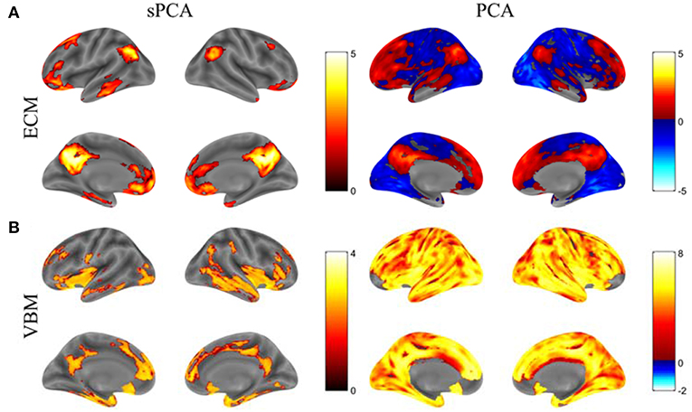
Figure 5. The standardized principal component maps having largest variance from sPCA and PCA. (A) ECM principal component, (B) VBM principal component.
Fusion Analysis
For each fusion method, the modulation profiles AECM and AVBM were calculated and two-sample t-tests with unequal variance were carried out to assess group difference. The ROC technique was applied on modulation profiles AECM and AVBM, and the AUC was calculated. Group classification accuracy was also calculated by running ten-fold quadratic discriminant analysis (QDA) on modulation profiles from both ECM and VBM modalities. The most significant component of AECM or AVBM from two-sample t-tests always had the largest AUC value. The AUC and Bonferroni-corrected p value for multiple comparisons, denoted as pcorr, of the most significant components are shown in Table 1. The correlation between the most significant components is also listed in this table. sPCA+CCA found one significant component in both ECM and VBM data (ECM: ; VBM: ). sPCA+CCA associated these two significant components at the 1st pair of canonical variates with canonical correlation ρ = 0.78. PCA+CCA found one significant component in both ECM and VBM data (; VBM: ). PCA+CCA associated these two significant components at the 1st pair of canonical variates with canonical correlation ρ = 0.48. Parallel ICA found one significant component in VBM but not in the ECM data (ECM: pcorr = 0.10, AUC = 0.68; VBM: ). The correlation between the most significant component in ECM and VBM was ρ = 0.27. sCCA found two significant ECM components and one VBM component (ECM: and ; VBM: ). The correlation between the most significant component in ECM and VBM was ρ = 0.80. Among these four fusion methods, sPCA+CCA achieved the highest group classification accuracy 0.68, which was more than 99-percentile of the null distribution. The classification accuracy with concatenated ECM and VBM principal component scores without fusion as input features to QDA was 0.57.
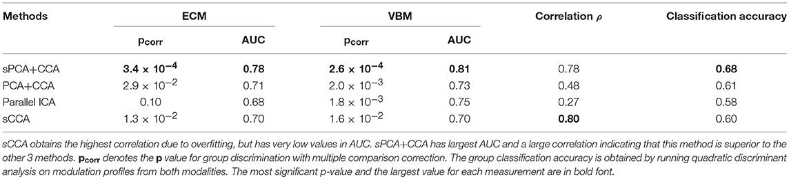
Table 1. Measurements of the modulation profiles in sPCA+CCA, PCA+CCA, parallel ICA and sCCA.
The spatial patterns for these four fusion methods were also computed for sPCA+CCA and PCA+CCA by using Equation (11). ECM z-score spatial patterns corresponding to the most significant components in AECM are shown in Figure 6. All spatial maps were thresholded at z ≥ 1.5 except the one from parallel ICA. The ECM spatial map from parallel ICA only showed an artifact on the brain boundary if thresholded at z ≥ 1.5, hence the threshold was lowered to z ≥ 1 for better interpretation. Anterior cingulate cortex (Bianciardi et al., 2009) was shown in the spatial patterns for all fusion methods. Both PCA+CCA and parallel ICA show some artifacts at the boundary of the brain. Bilateral superior temporal gyrus and bilateral amygdala were found in the ECM spatial pattern from sPCA+CCA.
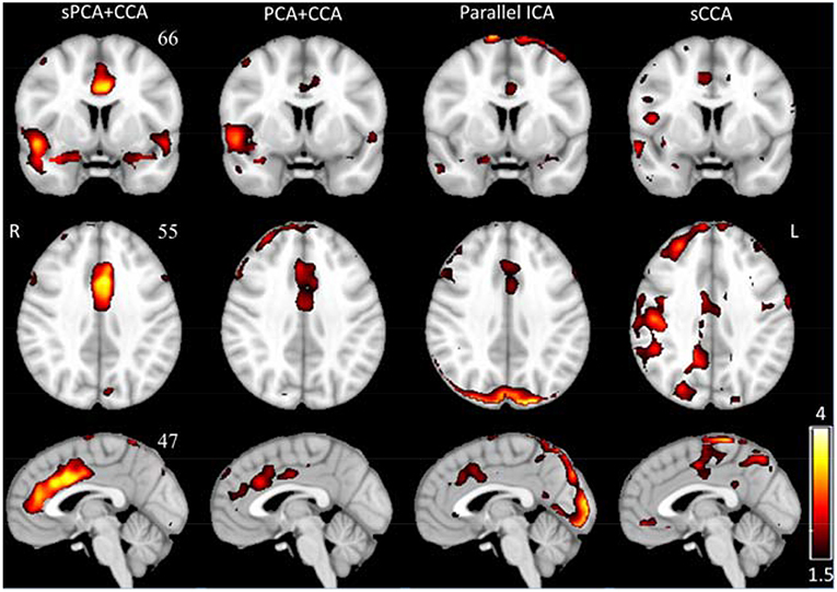
Figure 6. The most significant disease-related ECM z-score maps from sPCA+CCA, PCA+CCA, parallel ICA and sCCA. Maps are displayed in radiological convention (right is left and vice versa). All spatial maps are thresholded at z ≥ 1.5 except the map from parallel ICA that is thresholded at z ≥ 1. Parallel ICA would not show the anterior cingulate cortex if the map is thresholded at z ≥ 1.5.
VBM z-score maps corresponding to the most significant components in AVBM are shown in Figure 7. The spatial maps were thresholded at z ≥ 2. The VBM spatial maps are very similar except the one from PCA+CCA. In the VBM spatial maps, all fusion methods show gray matter atrophy in bilateral hippocampus and inferior temporal gyrus.
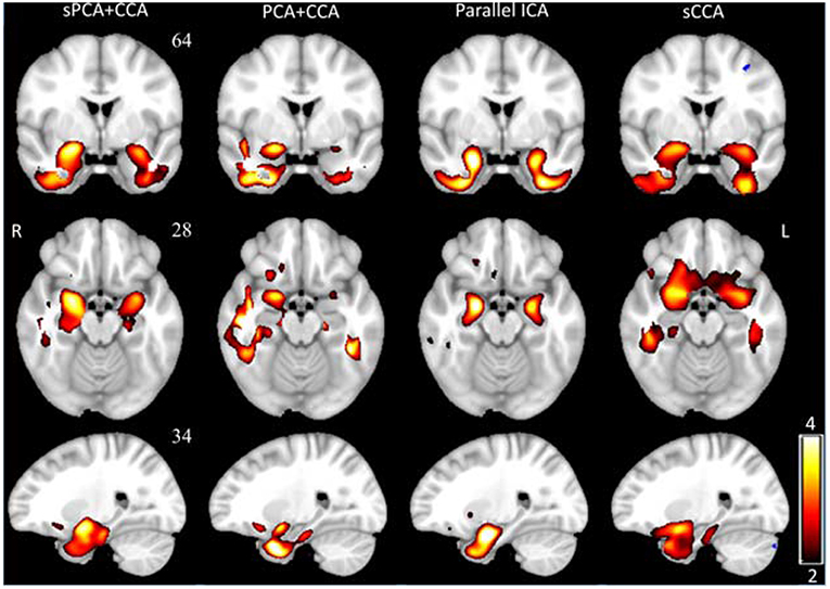
Figure 7. The most significant disease-related VBM z-score maps from sPCA+CCA, PCA+CCA, parallel ICA and sCCA. Maps are displayed in radiological convention (right is left and vice versa). All spatial maps were thresholded at z > 2. Note that PCA+CCA does not give a bilateral disease-related pattern.
Since the performance difference among these fusion methods shown in Figure 6 and Figure 7 may be affected by the number of remaining principal components, we have run sPCA+CCA, PCA+CCA and parallel ICA with the number of principal components ranging from 4 to 20 for both ECM and VBM datasets. For each fusion method, the most significant p-values for group discrimination with the number of principal components varying from 4 to 20 were recorded and the distribution of p-values is shown in Figure 8. The VBM datasets overall has more significant group difference than ECM datasets. Compared to PCA+CCA and parallel ICA, sPCA+CCA tends to have p-value more significant.
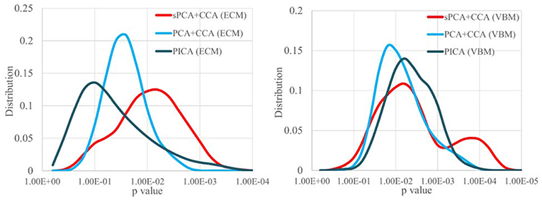
Figure 8. The distribution of p-values for group discrimination with the number of principal components ranging from 4 to 20. VBM dataset has more significant p-value than ECM dataset. The sPCA+CCA method has more significant group discrimination than PCA+CCA and parallel ICA.
Correlation Between Disease-Related Modulation Profiles and β-Amyloid Measurement
The most disease-related modulation profile in AECM and AVBM were correlated with SUVR, a measure of β-amyloid content calculated from the PET scans within 6 months of MRI scans. The correlation plots are shown in Figure 9. Each value in the ECM modulation profile measures the strength of functional connectivity for one subject, and a more negative value indicates lower functional connectivity. Similarly, each value in the VBM modulation profile measures the amount of atrophy for one subject, and a more negative value indicates more severe atrophy. Among these plots, only the VBM modulation profile in sPCA had a significant negative correlation with SUVR (p <0.05) and the other correlations were not significant. sPCA+CCA had the strongest correlation with SUVR in both ECM and VBM data.
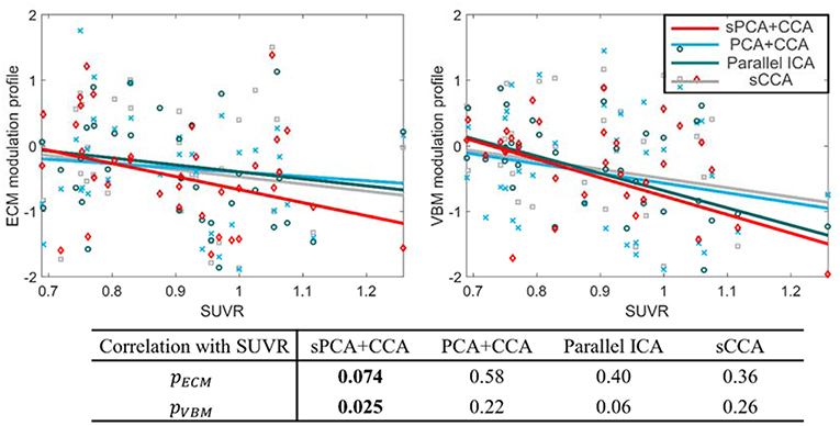
Figure 9. Correlation between the most significant modulation profiles in ECM and VBM modalities with SUVR. The significance p-values for ECM (pECM) and VBM data (pVBM) in sPCA+CCA, PCA+CCA, parallel ICA and sCCA are also shown. The SUVR measures the content of ß-amyloid using PET scanning. The ECM modulation profile of the disease-related pattern measures the strength of functional connectivity. A more negative value indicates lower functional connectivity. The VBM modulation profile of the disease-related pattern relates to the amount of atrophy. More atrophy is present for negative values of the VBM modulation profile. Note that sPCA+CCA has the most significant negative correlation with SUVR.
Discussion
To the best of our knowledge, our study is the first study proposing the sPCA+CCA method and comparing it with other methods for fusion analysis of multimodal brain imaging data. A novel split-sample cross-validation algorithm with AIC as selection criterion was validated for sPCA to determine the sparsity tuning parameter and the number of principal components. The sPCA+CCA fusion method extracts disease-related modulation profiles with the highest statistical power in real data. While sPCA and its variants were applied for noise elimination and functional segmentation in neuroimaging research (Ulfarsson and Solo, 2007; Ng et al., 2009; Khanna et al., 2015), to the best of our knowledge, this is the first study to implement and validate sPCA in fusion analysis.
Properties of sPCA
Since sPCA is a sparse version of PCA, naturally they have some common properties. Both are linear techniques for dimensionality reduction. High-dimensional data is projected to a subspace spanned by the dominant principal component scores so that most of the variance in the original data is kept in a low-dimensional feature space. However, sPCA is different from PCA in terms of robustness, implementation, orthogonality, and computation.
1) Robustness: sPCA not only searches for the direction to maximize variance but also discriminates informative voxels from non-informative voxels as a data-driven approach. In other words, sPCA is useful when the number of features is large, while only a small proportion of them are informative. In many cases the salient features such as age- and disease-related features in the modalities are limited to only a few regions but not the entire brain. The sPCA method adjusts principal components by setting non-informative voxels to zero and hence obtains more robust scores (projection of original data on principal components) as the input to the following CCA analysis. In the sPCA+CCA fusion method, sPCA itself does not have discriminatory power. However, it was shown that sPCA is more robust against noise than conventional PCA. The similarity values SY and SV in Figure 3 indicate that sPCA outperforms PCA in uncovering the true principal component scores and spatial maps, especially when the sparsity level is high. The robust scores from sPCA improve the subsequent CCA analysis to better link related modulation profiles and extract the corresponding spatial patterns in the data.
2) Implementation: Unlike PCA, which represents a standard eigenvalue problem, sPCA is a constrained optimization problem and optimized by an iterative algorithm. The objective function in sPCA is a biconvex function and is solved by optimizing two convex subproblems, both of which can be solved reliably and efficiently.
3) Orthogonality: The orthogonality no longer strictly holds when the L1 norm penalty term is added in sPCA. However, at the optimal sparsity tuning parameter, the mean absolute correlation with sign ignored between different principal components is 0.054, indicating that the principal components from sPCA are nearly orthogonal.
4) Computation: sPCA is more computationally intensive than standard PCA. Along with choosing the number of principal components as in PCA, sPCA also needs to specify the sparsity tuning parameter. Overestimated sparsity would be detrimental since informative voxels are also removed, and underestimated sparsity may not significantly improve the analysis. A grid search in PCA is carried out over the number of principal components, and a grid search in sPCA is carried out over a sparsity tuning parameter and the number of principal components. The grid search process exponentially increases computational time of sPCA because more parameters need to be optimized.
Comparison of Fusion Analysis
Fusion analysis was carried out with simulated and real data. In the simulations, the sPCA+CCA method has improved performance over PCA+CCA by about 10% at sparsity level 70%. We have tested these two fusion methods at different sparsity levels and found that the improvement decreases with lower sparsity level until the performance difference becomes negligible when the sparsity level is about 30%. We would like to point out that parallel ICA does not lead to orthogonal components because orthogonality is not strictly enforced unlike CCA-based fusion methods. Thus, the simulation generated with an orthogonality condition is biased toward CCA-based fusion methods and explains why parallel ICA does not perform well in our simulation. In contrast, generating data without the assumption of orthogonality would make the simulation more biased toward parallel ICA. Among the four fusion methods considered, sCCA overestimates the correlation between modalities and also has low similarity. Unlike sCCA having original voxel-wise input features, sPCA+CCA along with PCA+CCA and parallel ICA reduces the data dimension before fusing modalities and thus possibly may discard some correlated features that have low variance. The voxel-wise input features to sCCA, however, are much larger than the number of samples. For example, the number of non-zero features in sCCA is at the order of a thousand, while the number of input features to CCA in sPCA+CCA is of the order of ten. The elastic-net penalty as a sparsity constraint may not be sufficient to alleviate an overestimated canonical correlation relationship and thus sPCA+CCA still outperforms sCCA in both simulated and real data.
In real data, the proposed sPCA+CCA method has the most significant disease-related modulation profiles in both modalities and the highest group classification accuracy. Compared to the accuracy obtained with principal component scores as input, using the modulation profiles as input have improved classification accuracy for all considered fusion methods. ACC is found to be disease-related by all fusion methods in ECM data. A decreased functional connectivity of ACC was consistent with the findings in previous resting-state fMRI studies (Rombouts et al., 2005; Sheline et al., 2009) and ACC was also found to be affected in MCI subjects by other imaging techniques, such as single photon emission computed tomography (SPECT) and structural MRI studies (Huang et al., 2002; Karas et al., 2004). sPCA+CCA found that the amygdala and the superior temporal gyrus bilaterally, in addition to ACC, are important disease-related regions in the ECM data. Decreased functional connectivity of the amygdala and superior temporal gyrus in MCI or Alzheimer's disease subjects were also found in previous fMRI studies (Celone and Calhoun, 2006; Liu and Zhang, 2012; Yao et al., 2013), and are consistent with our results. In the VBM disease-related spatial maps, hippocampus and inferior temporal gyrus are found to have more atrophy in all fusion methods. The hippocampus is a critical region in the limbic system that is involved in motivation, emotion, learning and memory. Atrophy in the hippocampus is closely related to early symptoms in AD patients, such as short-term memory loss and disorientation. Early hippocampal atrophy is an established biomarker of AD (Jack et al., 1999). We also found that the inferior temporal gyrus is affected in MCI. This region is essential in face, pattern, and object recognition, and may already be affected in early-stage MCI subjects (Whitwell et al., 2008).
The disease-related modulation profiles from sPCA+CCA, PCA+CCA, parallel ICA and sCCA were correlated with the measure of β-amyloid, i.e., SUVR (Figure 9). Only sPCA+CCA found significant correlation with SUVR in VBM data but not in ECM data. The ECM modulation profile from sPCA+CCA, however, had strongest correlation with SUVR among all of ECM modulation profiles. A more negative value in the ECM modulation profile indicates lower functional connectivity, and a more negative value in the VBM modulation profile indicates more severe atrophy in the disease-related patterns. Since SUVR is used for longitudinal analyses in MCI (Landau et al., 2014), the disease-related spatial pattern and corresponding modulation profile from our fusion method potentially can be used to monitor disease severity.
Similar to other fusion methods, sPCA+CCA has its own assumptions and limitations. From the simulation and the formulation of sPCA+CCA, we illustrate that the CCA step enforces orthogonality on the modulation profile for each modality. In addition, implementing sparsity assumes that the associated effect between modalities is distributed locally instead of globally across the brain. This assumption is realistic because in amnestic MCI or early AD not the entire brain shows atrophy or loss of functional connectivity, but the disease state is limited to sparse brain regions such as the inferior temporal lobes and the posterior cingulate cortex. Enforcing sparsity in fusion analysis is applicable to many neurological diseases in their early stages. On a computational level, enforcing sparsity significantly increases computational time. Computations were run on a Dell workstation with 2 Intel Xeon E5-2643 processors. This is different from parallel ICA and PCA+CCA, where the computation takes only minutes to carry out a fusion analysis. In contrast, sPCA+CCA needs approximately 12 h to complete the analysis, and sCCA needs ~21 h.
Extension of sPCA+CCA
We would like to emphasize that sPCA also can be applied to other CCA-based fusion methods such as multiset CCA (Correa et al., 2010) and CCA+jICA (Sui et al., 2010, 2011). Unlike CCA that associates only two modalities, multiset CCA is applied when more than two modalities are considered for fusion analysis. In the CCA+jICA method, joint ICA is carried out after CCA to maximize the independence among joint components and to prevent CCA from failing to separate sources. Since PCA is also required in these two methods for dimensionality reduction, sPCA can be incorporated into these methods as well. If the structural information in the brain map is pre-specified, more sophisticated sparse constraints such as structural lasso (Simon et al., 2013; Lin et al., 2014) can potentially be used in sparse fusion methods including sPCA+CCA and sCCA. However, more advanced methods are beyond the scope of the current study.
Limitations and Future Study
The proposed sPCA method has two limitations. First, as in PCA, sPCA preserves the global structure of the data but ignores the Euclidean structure of image space and hence may lead to discrete non-zero voxels in sparse principal components. Second, the property of orthogonality between principal components does not strictly hold because of the lasso penalty used in sPCA. Furthermore, the issue of missing data is not addressed in this study. Some subjects may only have one imaging modality available or have data with partial brain coverage, while some fusion methods have been developed to address this issue (Xiang et al., 2014; Pan et al., 2018), current sPCA+CCA framework cannot use subjects with missing data.
Other dimension reduction methods, such as the locality preserving projection method (He and Niyogi, 2003), were studied extensively in pattern recognition. However, the performance of more sophisticated dimension reduction techniques for neuroimaging studies is unknown. The auto encoder related methods (Bengio, 2009) are currently of high interest in the deep learning research community. This method is appealing for handling non-linear systems and could replace the linear PCA algorithm. One critical reason for requiring dimension reduction in CCA-based fusion analysis is that the number of features in standard CCA algorithm cannot be more than the number of observations. If CCA itself can be revised to select features adaptively and avoid the singularity problem arising from too many features, then the dimension reduction preprocessing step may not be required.
Conclusion
We have proposed a sPCA algorithm for data fusion and compared sPCA with three different state-of-the-art fusion methods. We evaluated how well these fusion methods associate related patterns in different modalities and correlated the result from fusion analysis with ß-amyloid measurement (SUVR). We found that sPCA can significantly reduce the impact of non-informative voxels and improve statistical power for uncovering disease-related patterns. The sPCA+CCA method not only achieves the best group discrimination but also has the strongest correlation with the SUVR measurement. In summary, sPCA is a powerful method for sparse regularization and dimensionality reduction, completely data-driven, and self-adaptive without experts' intervention.
Author Contributions
ZY and DC: conception and design of the study. ZY, XZ, KS, VM, SB, and DC: analysis and interpretation of data. CB: data management and quality control. DC and ZY: drafting the article. ZY, XZ, CB, KS, VM, SB, and DC: revising it critically for important intellectual content and final approval of the version to be submitted.
Funding
This research project was supported by the NIH (grant 1R01EB014284 and COBRE grant 5P20GM109025), a private grant from Angela and Peter Dal Pezzo, and a private grant from Lynn and William Weidner. Data collection and sharing for this project was funded by the ADNI (National Institutes of Health Grant U01 AG024904) and DOD ADNI (Department of Defense award number W81XWH-12-2-0012).
Conflict of Interest Statement
The authors declare that the research was conducted in the absence of any commercial or financial relationships that could be construed as a potential conflict of interest.
Supplementary Material
The Supplementary Material for this article can be found online at: https://www.frontiersin.org/articles/10.3389/fnins.2019.00642/full#supplementary-material
References
Abdel-Rahman, E. M., Mutanga, O., Odindi, J., Adam, E., Odindo, A., and Ismail, R. (2014). A comparison of partial least squares (PLS) and sparse PLS regressions for predicting yield of Swiss chard grown under different irrigation water sources using hyperspectral data. Comput. Electron. Agric. 106, 11–19. doi: 10.1016/j.compag.2014.05.001
Akaike, H. (1974). A new look at the statistical model identification. IEEE Trans. Automat. Control 19, 716–723. doi: 10.1109/TAC.1974.1100705
Ashburner, J. (2007). A fast diffeomorphic image registration algorithm. Neuroimage 38, 95–113. doi: 10.1016/j.neuroimage.2007.07.007
Ashburner, J., and Friston, K. J. (2000). Voxel-based morphometry—the methods. Neuroimage 11, 805–821. doi: 10.1006/nimg.2000.0582
Avants, B. B., Libon, D. J., Rascovsky, K., Boller, A., McMillan, C. T., Massimo, L., et al. (2014). Sparse canonical correlation analysis relates network-level atrophy to multivariate cognitive measures in a neurodegenerative population. Neuroimage 84, 698-711. doi: 10.1016/j.neuroimage.2013.09.048
Bai, F., Watson, D. R., Yu, H., Shi, Y., Yuan, Y., and Zhang, Z. (2009). Abnormal resting-state functional connectivity of posterior cingulate cortex in amnestic type mild cognitive impairment. Brain Res. 1302, 167–174. doi: 10.1016/j.brainres.2009.09.028
Bavelas, A. (1948). A mathematical model for group structures. Hum. Org. 7, 16–30. doi: 10.17730/humo.7.3.f4033344851gl053
Bengio, Y. (2009). Learning deep architectures for AI. Found. Trends® Mach. Learn. 2, 1–127. doi: 10.1561/2200000006
Bianciardi, M., Fukunaga, M., van Gelderen, P., Horovitz, S. G., de Zwart, J. A., Shmueli, K., et al. (2009). Sources of functional magnetic resonance imaging signal fluctuations in the human brain at rest: a 7 T study. Magnet. Reson. Imag. 27, 1019–1029. doi: 10.1016/j.mri.2009.02.004
Bryan, K., and Leise, T. (2006). The $25,000,000,000 eigenvector: The linear algebra behind Google. Siam Rev. 48, 569–581. doi: 10.1137/050623280
Calhoun, V. D., and Adal, T. (2009). Feature-based fusion of medical imaging data. IEEE Trans. Info. Technol. Biomed. 13, 711–720. doi: 10.1109/TITB.2008.923773
Calhoun, V. D., and Sui, J. (2016). Multimodal fusion of brain imaging data: a key to finding the missing link (s) in complex mental illness. Biol. Psychiatry Cogn. Neurosci. Neuroimaging 1, 230–244. doi: 10.1016/j.bpsc.2015.12.005
Celone, K. A.Calhoun, V. D., et al. (2006). Alterations in memory networks in mild cognitive impairment and Alzheimer's Disease: an independent component analysis. J. Neurosci. 26 10222–10231. doi: 10.1523/JNEUROSCI.2250-06.2006
Chen, J. E., Chang, C., Greicius, M. D., and Glover, G. H. (2015). Introducing co-activation pattern metrics to quantify spontaneous brain network dynamics. Neuroimage 111, 476–488. doi: 10.1016/j.neuroimage.2015.01.057
Chetelat, G., Desgranges, B., De La Sayette, V., Viader, F., Eustache, F., and Baron, J.-C. (2002). Mapping gray matter loss with voxel-based morphometry in mild cognitive impairment. Neuroreport 13, 1939–1943. doi: 10.1097/00001756-200210280-00022
Correa, N. M., Adali, T., Li, Y. O., and Calhoun, V. D. (2010). Canonical correlation analysis for data fusion and group inferences: examining applications of medical imaging data. IEEE Sig. Process Mag. 27, 39–50. doi: 10.1109/MSP.2010.936725
Correa, N. M., Li, Y. O., Adali, T., and Calhoun, V. D. (2008). Canonical correlation analysis for feature-based fusion of biomedical imaging modalities and its application to detection of associative networks in Schizophrenia. IEEE J Sel Top Signal Proc. 2, 998–1007. doi: 10.1109/JSTSP.2008.2008265
Eckart, C., and Young, G. (1936). The approximation of one matrix by another of lower rank. Psychometrika 1, 211–218. doi: 10.1007/BF02288367
Feng, C. M., Gao, Y. L., Liu, J. X., Zheng, C. H., Li, S. J., and Wang, D. (2016). “A simple review of sparse principal components analysis,” in International Conference on Intelligent Computing (Springer), 374–383.
Filippi, M., Cercignani, M., Inglese, M., Horsfield, M., and Comi, G. (2001). Diffusion tensor magnetic resonance imaging in multiple sclerosis. Neurology 56, 304–311. doi: 10.1212/WNL.56.3.304
Forsberg, A., Engler, H., Almkvist, O., Blomquist, G., Hagman, G., Wall, A., et al. (2008). PET imaging of β-amyloid deposition in patients with mild cognitive impairment. Neurobiol. Aging 29, 1456–1465. doi: 10.1016/j.neurobiolaging.2007.03.029
Fulop, S. A., and Fitz, K. (2006). Algorithms for computing the time-corrected instantaneous frequency (reassigned) spectrogram, with applications. J. Acoust. Soc. Am. 119, 360–371. doi: 10.1121/1.2133000
Groves, A. R., Beckmann, C. F., Smith, S. M., and Woolrich, M. W. (2011). Linked independent component analysis for multimodal data fusion. Neuroimage 54, 2198–2217. doi: 10.1016/j.neuroimage.2010.09.073
He, X., and Niyogi, P. (2003). “Locality preserving projections,” in Advances in Neural Information Processing Systems 16 (Vancouver, BC).
He, Y., and Evans, A. (2010). Graph theoretical modeling of brain connectivity. Curr. Opin. Neurol. 23, 341–350. doi: 10.1097/WCO.0b013e32833aa567
Henson, R. N., Flandin, G., Friston, K. J., and Mattout, J. (2010). A Parametric empirical bayesian framework for fMRI-constrained MEG/EEG source reconstruction. Hum. Brain Mapp. 31, 1512–1531. doi: 10.1002/hbm.20956
Hotelling, H. (1936). Relations between two sets of variates. Biometrika 28, 321–377. doi: 10.1093/biomet/28.3-4.321
Huang, C., Wahlund, L. O., Svensson, L., Winblad, B., and Julin, P. (2002). Cingulate cortex hypoperfusion predicts Alzheimer's disease in mild cognitive impairment. BMC Neurol. 2:9. doi: 10.1186/1471-2377-2-9
Jack, C. R., Petersen, R. C., Xu, Y. C., O'Brien, P. C., Smith, G. E., Ivnik, R. J., et al. (1999). Prediction of AD with MRI-based hippocampal volume in mild cognitive impairment. Neurology 52, 1397–1397. doi: 10.1212/WNL.52.7.1397
Jenatton, R., Obozinski, G., and Bach, F. (2010). “Structured sparse principal component analysis,” in Proceedings of the Thirteenth International Conference on Artificial Intelligence and Statistics (Paris), 366–373.
Karas, G. B., Scheltens, P., Rombouts, S. A. R. B., Visser, P. J., van Schijindel, R. A., Fox, N. C., et al. (2004). Global and local gray matter loss in mild cognitive impairment and Alzheimer's disease. Neuroimage 23, 708–716. doi: 10.1016/j.neuroimage.2004.07.006
Khanna, R., Ghosh, J., Poldrack, R., and Koyejo, O. (2015). Sparse submodular probabilistic PCA. Art. Intell. Statist. 38, 453–461.
Kim, D., Ronen, I., Formisano, E., Kim, K., Kim, M., van Zijl, P., et al. (2003). Simultaneous Mapping of Functional Maps and Axonal Connectivity in Cat Visual Cortex. Sendai: HBM.
Lê Cao, K.-A., Boitard, S., and Besse, P. (2011). Sparse PLS discriminant analysis: biologically relevant feature selection and graphical displays for multiclass problems. BMC Bioinformatics 12:253. doi: 10.1186/1471-2105-12-253
Lameiro, C., and Schreier, P. J. (2016). Cross-Validation Techniques for Determing the Number of Correlated Components Between Two Data When the Number of Sampls is Very Small. Pacific Grove, CA: ICASSP.
Landau, S. M., Baker, S. L., and Jagust, W. J. (2014). “Amyloid change early in disease is related to increased glucose metabolism and episodic memory declinein,” in Human Amyloid Imaging Meeting (Miami, FL).
Le Floch, E., Guillemot, V., Frouin, V., Pinel, P., Lalanne, C., Trinchera, L., et al. (2012). Significant correlation between a set of genetic polymorphisms and a functional brain network revealed by feature selection and sparse partial least squares. Neuroimage 63, 11–24. doi: 10.1016/j.neuroimage.2012.06.061
Lin, D., Calhoun, V. D., and Wang, Y. (2014). Correspondence between fMRI and SNP data by group sparse canonical correlation analysis. Med. Image Anal. 18, 891–902. doi: 10.1016/j.media.2013.10.010
Liu, J., Pearlson, G., Windemuth, A., Ruano, G., Perrone-Bizzozero, N. I., and Calhoun, V. (2009). Combining fMRI and SNP data to investigate connections between brain function and genetics using parallel ICA. Hum. Brain Mapp. 30, 241–255. doi: 10.1002/hbm.20508
Liu, Z.Zhang, Y., et al. (2012). Altered topological patterns of brain networks in mild cognitive impairment and Alzheimer's disease: a resting-state fMRI study. Psychiatr. Res. Neuroimaging. 202, 118–125. doi: 10.1016/j.pscychresns.2012.03.002
Mohammadi-Nejad, A. R., Hossein-Zadeh, G. A., and Soltanian-Zadeh, H. (2017). Structured and sparse canonical correlation analysis as a brain-wide multi-modal data fusion approach. IEEE. Trans. Med. Imag. 11, 1–11. doi: 10.1109/TMI.2017.2681966
Ng, B., Abugharbieh, R., and McKeown, M. (2009). Functional segmentation of fMRI data using adaptive non-negative sparse PCA (ANSPCA). Med. Image Comput. Comp. Assis. Interven. 2009, 490–497. doi: 10.1007/978-3-642-04271-3_60
Pan, Y., Liu, M., Lian, C., Zhou, T., Xia, Y., and Shen, D. (2018). “Synthesizing missing PET from MRI with cycle-consistent generative adversarial networks for Alzheimer's disease diagnosis,” in International Conference on Medical Image Computing and Computer-Assisted Intervention (Granada: Springer), 455–463. doi: 10.1007/978-3-030-00931-1_52
Parkhomenko, E., Tritchler, D., and Beyene, J. (2009). Sparse canonical correlation analysis with application to genomic data integration. Stat. Appl. Genet. Mol. Biol. 8, 1–34. doi: 10.2202/1544-6115.1406
Pezeshki, A., Scharf, L. L., Azimi-Sadjadi, M. R., and Lundberg, M. (2004). “Empirical canonical correlation analysis in subspaces,” in Signals, Systems and Computers, (2004). Conference Record of the Thirty-Eighth Asilomar Conference on (Pacific Grove, CA: IEEE), 994–997.
Power, J. D., Cohen, A. L., Nelson, S. M., Wig, G. S., Barnes, K. A., Church, J. A., et al. (2011). Functional network organization of the human brain. Neuron 72, 665–678. doi: 10.1016/j.neuron.2011.09.006
Rombouts, S. A. R. B., Barkhof, F., Goekoop, R., Stam, C. J., and Scheltens, P. (2005). Altered resting state networks in mild cognitive impairment and mild Alzheimer's disease: An fMRI study. Hum. Brain Mapp. 26, 231–239. doi: 10.1002/hbm.20160
Savopol, F., and Armenakis, C. (2002). Merging of heterogeneous data for emergency mapping: data integration or data fusion? Int. Arch. Photogramm. Remote Sens. Spatial Info. Sci. 34, 668–674.
Sheline, Y. I., Raichle, M. E., Snyder, A. Z., Morris, J. C., Head, D., Wang, S., et al. (2009). Amyloid plaques disrupt resting state default mode network connectivity in cognitively normal elderly. Biol. Psychiatr. 67:584–587. doi: 10.1016/j.biopsych.2009.08.024
Shen, H., and Huang, J. Z. (2008). Sparse principal component analysis via regularized low rank matrix approximation. J. Multivar. Anal. 99, 1015–1034. doi: 10.1016/j.jmva.2007.06.007
Shumway, R. H., Stoffer, D. S., and Stoffer, D. S. (2000). Time Series Analysis and Its Applications. New York, NY: Springer.
Simon, N., Friedman, J., Hastie, T., and Tibshirani, R. (2013). A sparse-group lasso. J. Comput. Graph. Stat. 22, 231–245. doi: 10.1080/10618600.2012.681250
Sui, J., Adali, T., Pearlson, G., Yang, H., Sponheim, S. R., White, T., et al. (2010). A CCA+ICA based model for multi-task brain imaging data fusion and its application to schizophrenia. Neuroimage 51, 123–134. doi: 10.1016/j.neuroimage.2010.01.069
Sui, J., Pearlson, G., Caprihan, A., Adali, T., Kiehl, K. A., Liu, J., et al. (2011). Discriminating schizophrenia and bipolar disorder by fusing fMRI and DTI in a multimodal CCA+ joint ICA model. Neuroimage 57, 839–855. doi: 10.1016/j.neuroimage.2011.05.055
Troyanskaya, O., Cantor, M., Sherlock, G., Brown, P., Hastie, T., Tibshirani, R., et al. (2001). Missing value estimation methods for DNA microarrays. Bioinformatics 17, 520–525. doi: 10.1093/bioinformatics/17.6.520
Ulfarsson, M. O., and Solo, V. (2007). “Sparse variable principal component analysis with application to fMRI. Biomedical Imaging: From Nano to Macro, 2007,” in 4th IEEE International Symposium on IEEE, ISBI 2007 (Arlington, VA), 460–463.
Whitwell, J. L., Shiung, M. M., Przybelski, S., Weigand, S. D., Knopman, D. S., Boeve, B. F., et al. (2008). MRI patterns of atrophy associated with progression to AD in amnestic mild cognitive impairment. Neurology 70, 512–520. doi: 10.1212/01.wnl.0000280575.77437.a2
Wink, A. M., de Munck, J. C., van der Werf, Y. D., van den Heuvel, O. A., and Barkhof, F. (2012). Fast eigenvector centrality mapping of voxel-wise connectivity in functional magnetic resonance imaging: implementation, validation, and interpretation. Brain connectivity 2, 265–274. doi: 10.1089/brain.2012.0087
Witten, D. M., Tibshirani, R., and Hastie, T. (2009). A penalized matrix decomposition, with applications to sparse principal components and canonical correlation analysis. Biostatistics 10, 515–534. doi: 10.1093/biostatistics/kxp008
Witten, D. M., and Tibshirani, R. J. (2009). Extensions of sparse canonical correlation analysis with applications to genomic data. Stat. Appl. Genet. Mol. Biol. 8, 1–27. doi: 10.2202/1544-6115.1470
Xiang, S., Yuan, L., Fan, W., Wang, Y., Thompson, P. M., Ye, J., et al. (2014). Bi-level multi-source learning for heterogeneous block-wise missing data. Neuroimage 102, 192–206. doi: 10.1016/j.neuroimage.2013.08.015
Yao, H., Liu, Y., Zhou, B., Zhang, Z., An, N., Wang, P., et al. (2013). Decreased functional connectivity of the amygdala in Alzheimer's disease revealed by resting-state fMRI. Eur J Radiol. 82, 1531–1538. doi: 10.1016/j.ejrad.2013.03.019
Keywords: sparse principal component analysis, PCA, canonical correlation analysis, CCA, data fusion, mild cognitive impairment, MCI
Citation: Yang Z, Zhuang X, Bird C, Sreenivasan K, Mishra V, Banks S, Cordes D and the Alzheimer's Disease Neuroimaging Initiative (2019) Performing Sparse Regularization and Dimension Reduction Simultaneously in Multimodal Data Fusion. Front. Neurosci. 13:642. doi: 10.3389/fnins.2019.00642
Received: 14 January 2019; Accepted: 04 June 2019;
Published: 03 July 2019.
Edited by:
Daoqiang Zhang, Nanjing University of Aeronautics and Astronautics, ChinaReviewed by:
Babak A. Ardekani, Nathan Kline Institute for Psychiatric Research, United StatesMingxia Liu, University of North Carolina at Chapel Hill, United States
Copyright © 2019 Yang, Zhuang, Bird, Sreenivasan, Mishra, Banks, Cordes and the Alzheimer's Disease Neuroimaging Initiative. This is an open-access article distributed under the terms of the Creative Commons Attribution License (CC BY). The use, distribution or reproduction in other forums is permitted, provided the original author(s) and the copyright owner(s) are credited and that the original publication in this journal is cited, in accordance with accepted academic practice. No use, distribution or reproduction is permitted which does not comply with these terms.
*Correspondence: Dietmar Cordes, Y29yZGVzZEBjY2Yub3Jn
†Data used in preparation of this article were obtained from the Alzheimer's Disease Neuroimaging Initiative (ADNI) database (http://adni.loni.usc.edu/). As such, the investigators within the ADNI contributed to the design and implementation of ADNI and/or provided data but did not participate in analysis or writing of this report. A complete listing of ADNI investigators can be found at https://adni.loni.usc.edu/wp-content/uploads/how_to_apply/ADNI_Acknowledgement_List.pdf