 Nicole H. Yuen
 Nathaniel Osachoff
 J. Jean Chen
- 1Rotman Research Institute at Baycrest, Toronto, ON, Canada
- 2Department of Medical Biophysics, University of Toronto, Toronto, ON, Canada
The frequency characteristics of the resting-state BOLD fMRI (rs-fMRI) signal are of increasing scientific interest, as we discover more frequency-specific biological interpretations. In this work, we use variational mode decomposition (VMD) to precisely decompose the rs-fMRI time series into its intrinsic mode functions (IMFs) in a data-driven manner. The accuracy of the VMD decomposition of constituent IMFs is verified through simulations, with higher reconstruction accuracy and much-reduced mode mixing relative to previous methods. Furthermore, we examine the relative contribution of the VMD-derived modes (frequencies) to the rs-fMRI signal as well as functional connectivity measurements. Our primary findings are: (1) The rs-fMRI signal within the 0.01–0.25 Hz range can be consistently characterized by four intrinsic frequency clusters, centered at 0.028 Hz (IMF4), 0.080 Hz (IMF3), 0.15 Hz (IMF2) and 0.22 Hz (IMF1); (2) these frequency clusters were highly reproducible, and independent of rs-fMRI data sampling rate; (3) not all frequencies were associated with equivalent network topology, in contrast to previous findings. In fact, while IMF4 is most likely associated with physiological fluctuations due to respiration and pulse, IMF3 is most likely associated with metabolic processes, and IMF2 with vasomotor activity. Both IMF3 and IMF4 could produce the brain-network topology typically observed in fMRI, whereas IMF1 and IMF2 could not. These findings provide initial evidence of feasibility in decomposing the rs-fMRI signal into its intrinsic oscillatory frequencies in a reproducible manner.
Introduction
The frequency characteristics of the resting-state BOLD fMRI (rs-fMRI) signal are of increasing scientific interest (Salvador et al., 2005; Niazy et al., 2011; Kalcher et al., 2014), as we discover more frequency-specific biological interpretations within the conventional data-acquisition bandwidth of 0–0.25 Hz (Golestani et al., 2015; Hocke et al., 2016). In particular, specific spectral content have been associated with physiological and vascular processes (Birn et al., 2008; Golestani et al., 2015; Mark et al., 2015; Hocke et al., 2016) and with the resulting brain-network measures (Nikolaou et al., 2016). Thus, spectral analysis of the rs-fMRI signal appears to be a compelling approach to achieving a better appreciation of how much neurally relevant information is conveyed by rs-fMRI. To that end, band-pass filtering has been used in the initial efforts (Kalcher et al., 2014). However, in theory, the rs-fMRI signal does not lend itself to conventional band-pass filtering approaches, as it is not stationary and cannot be defined by a few frequencies in Fourier domain. The band-pass filtering approach is inadequate for studying non-stationary signals, as the frequency content of such signals changes with time, while a filter bank is limited by assumptions regarding frequency, bandwidths and the type of filter design.
Previous studies examining the frequency characteristics of the resting-state BOLD fMRI (rs-fMRI) signal were largely based on the decomposition of the rs-fMRI signal into its intrinsic mode functions (IMFs). Existing studies (Niazy et al., 2011; Song et al., 2014) have used empirical mode decomposition (EMD) (Huang et al., 1998) and later used complementary ensemble empirical mode decomposition (CEEMD) (Wu and Huang, 2009; Yeh et al., 2012; Qian et al., 2015). At the core of EMD and CEEMD is a simple workflow. Signal local minima and maxima are recursively detected, based on which an upper and lower envelope are obtained through interpolation; subsequently, the midline of the resultant envelope is removed and the high-frequency component becomes the IMF. The same process is then performed on the signal composed of the low-frequency midline. Thus, each IMF can be expressed as a combination of a low-frequency amplitude-modulated and a high-frequency frequency-modulated signal Eq. (1),
Where ∅(t) modulates the carrier frequency. The total bandwidth of this signal is described by Eq. (2),
where Δf is the total deviation from the instantaneous frequency of the IMF, while fFM represents the maximum rate of the change of the instantaneous frequency, and fAM represent the highest frequency of the envelope modulating the frequency-modulated signal. The IMF frequency estimate could be dominated by either of these, depending on noise conditions.
Previous works using EMD and CEEMD have both found that the rs-fMRI can be approximated by 4 to 5 IMFs covering the entire sampling bandwidth (Niazy et al., 2011; Qian et al., 2015), and that all IMFs can be used to reproduce similar network topologies. A fundamental assumption of EMD and its derivatives is that each IMF occupies a well-defined frequency range (Huang et al., 1998). In theory, the IMF-based representation is insensitive to non-stationarity and non-linearity in the original signal. EMD-type approaches are known to have difficulty separating tones of similar frequencies. Moreover, high levels of non-white noise can interfere with the accurate identification of the instantaneous frequency, and cause the frequency to appear to shift in a non-linear fashion, leading to mode mixing between IMFs (Wu and Huang, 2009) as well as the same mode to be spread across multiple IMFs. In addition, EMD-derived methods have a tendency to attribute wider bandwidths to IMFs occupying higher frequencies. This is likely a result of the recursions, which present the highest degree of uncertainty to the first (highest-frequency) IMFs, and not allowing for backward error correction after subsequent IMFs have been extracted. Indeed, when applied to rs-fMRI data, CEEMD resulted in visible modal widening as frequency increased (Qian et al., 2015).
Our study incorporates the usage of the recently proposed variational mode decomposition (VMD) method (Dragomiretskiy and Zosso, 2014) to decompose the BOLD rs-fMRI time series into its IMFs. Recently, the VMD method has recently found application in the analysis of geological signals (Liu et al., 2016; Xiao et al., 2016) and electrocardiographic data (Lahmiri, 2014; Mert, 2016; Tripathy et al., 2016). The theory of VMD has been described in detail elsewhere (Dragomiretskiy and Zosso, 2014), and will not be repeated here. We will simply point out that unlike its predecessors, VMD is non-recursive, and can reconstruct all modes simultaneously, controlled by a convergence criterion. The variational model assesses the bandwidth of the modes by minimizing the Gaussian-regularized mean-square error between the signal and its representation as a series of Wiener filters, with the modal instantaneous frequency being determined as the center of mass of the power-spectral density function of each IMF. This approach increases the robustness of the model to estimation uncertainties. VMD provides error checking, as the VMD solution is be updated by minimizing the mean-squared residual of all IMFs against the estimate of any given IMF. Lastly, the VMD convergence depends on a series of iterative optimizations, during which the balance between overfitting and signal-estimation accuracy can be adjusted, for instance, based on a priori knowledge about the signal.
In this work, we hypothesize that VMD is able to more precisely extract frequency bands from the rs-fMRI signal, reducing the issue of mode mixing and mode spreading demonstrated in the previous work. To verify this hypothesis, we tested the EMD, CEEMD, and VMD techniques through a Monte Carlo simulation. Furthermore, although prior work (using EMD and CEEMD) have suggested that resting-state networks (RSNs) measured through rs-fMRI are frequency independent, we hypothesize that existing results are affected by modal mixing and limited frequency precision as described herein. To address this hypothesis, we re-examine the frequency dependence of functional connectivity of RSNs using VMD.
Materials and Methods
VMD Optimization
As documented in the original paper, the VMD technique follows three steps: (1) estimate individual IMFs by computing the Hilbert transform of the original signal f; (2) shift each mode to its base frequency using heterodyne demodulation; (3) estimate the bandwidth of each mode as the H1 Gaussian smoothness of the demodulated signal. The target for the decomposition should be that
where k is the number of IMFs. If the signal f is smooth, the solution could be obtained through Tikhonov regularized minimization,
where f0 is the measured signal, f is the original (clean) signal, and α is the regularization parameter. From this, we obtained the Euler-Lagrange equation:
where (δtt is the partial derivative with respect to time and is the frequency in radians.
The minimization target of the VMD algorithm can be summarized by Eq. 6, which describes the inverse of the Gaussian smoothness of the demodulated signal,
where (δ(t) is Dirac’s delta function, is the Euclidean norm squared, and j (=(v−1. This is solved using the augmented Lagrangian:
where
where (λ is the Langragian multiplier, b is the quadratic penalty term (squared residual) and c is the inner product of and the residual. The solution to the original variational problem is solved as the saddle point of the augmented Lagrangian. Each IMF is updated iteratively (by solving the VMD problem with respect to u and to ω until convergence is reached. In this way, all modes are extracted and optimized concurrently instead of sequentially.
In this study, we explicitly optimized the value of the regularization parameter α to balance the bandwidths of the spectral bands and the reconstruction error between the sum of the bands and the original signal. This parameter was chosen to minimize the overlap between the spectral bands in the Fourier domain while keeping the parameter as low as possible to retain reconstruction fidelity.
Simulated Data
To compare the performance of the VMD method in relation to EMD and CEEMD methods, we performed a Monte Carlo simulation involving a known, “ground-truth” signal. First, we generated a signal composed of equal power contributions from four frequencies (0.03, 0.08, 0.15, and 0.23 Hz). This signal was sampled at 0. 25 Hz to emulate the typical sampling rate of rs-fMRI data (TR = 2 s), and the constituent frequencies were informed in part by those previously reported (Niazy et al., 2011; Qian et al., 2015). We then generated 200 variants of signal-noise mixtures, in which 200 different realizations of white noise time series were added to the signal to achieve a signal-to-noise ratio (SNR) of ∼1.2. This is representative of the lower end of the realistic SNR range in rs-fMRI data, particularly to accommodate the fact that the spectral signature of noise in real rs-fMRI data is imprecise and non-stationary. All three decomposition methods were then applied to extract the original frequencies. To quantify the performances of the different algorithms, we computed the fractional inter-modal overlap (mode mixing) for each, defined as the amount of spectral power in the neighboring IMFs as a fraction of the total spectral power of each “ground-truth” IMF.
MRI Data Acquisition
MRI data were collected from 8 healthy adults (mean age 30 ± 6.7 years) on a 3T Siemens TIM Trio scanner and a 32-channel head coil. Specifically, whole-brain resting-state fMRI (rs-fMRI) data were acquired using single-shot gradient-echo EPI. The conventional-TR scans are later referred as “long-TR” scans: 26 slices, TR = 2 s, flip angle = 70°, FOV = 220 mm × 200 mm, voxel size = 3.4 mm × 3.4 mm × 4.6 mm in 240 frames. To enable assessment of reproducibility of our methods, the rs-fMRI scan was performed twice for each subject (two trials per subject) within the same session. On a subset of seven subjects, we also acquired rs-fMRI data using simultaneous multi-slice (SMS) acceleration on the gradient-echo EPI (Feinberg et al., 2010) (TR = 323 ms, TE = 30 ms, flip angle = 40°, 15 slices, 3.44 mm × 3.44 mm × mm, 2230 time points, acceleration factor = 3, phase encoding shift factor = 2, slices ascending). The brain coverage of these “short-TR” scans was matched to that of the “long-TR” scans, and we only used 1486 frames of the short-TR scans for comparison with the long-TR scan results. This would permit us to assess the dependence of our results to fMRI sampling rate. A 3D T1-weighted anatomical scan was acquired using MPRAGE, with resolution 1 × 1 × 1 mm, repetition time (TR) = 2400 ms, inversion time (TI) = 1000 ms, echo time (TE) = 2.43 ms, flip angle = 8, field of view × 256 × 256 mm (sagittal), matrix size = 256 × 256, 192 slices (ascending order), bandwidth = 180 Hz/pixel, and GRAPPA acceleration factor = 2.
Image Preprocessing
The rs-fMRI data were preprocessed using FSL FEAT version 5.0.8 (Jenkinson et al., 2002). Functional data had the first 10 volumes removed and skull stripped using the Brain Extraction Tool (BET). Data were corrected for motion (reference being the middle frame of each data set) and slice time then band-pass filtered to be between 0.01 and 0.25 Hz (using fslmaths, which implements a Gaussian filter). The cut-off of 0.25 Hz was chosen to represent the maximum detectable frequency in typical rs-fMRI acquisitions (i.e., TR = 2 s). Similar to prior work of a similar nature (Niazy et al., 2011; Tong et al., 2011), we did not actively correct physiological artifacts. The VMD technique was then used to decompose the preprocessed BOLD signal, and the results were compared to those obtained using the EMD and CEEMD methods.
The T1 anatomical scans were used in defining noise regions of interest (ROIs) for further analysis. Specifically, we used FMRIB Automated Segmentation Tool (FAST) for segmentation of gray matter, white matter, and cerebrospinal fluid ROIs. The FSL-FAST segmentation routine is based on a Hidden Markov Random Field model that is optimized using the expectation-maximization algorithm (Zhang et al., 2001). The ROI masks are then aligned with the fMRI data using anatomical-to-fMRI transformation matrices determined using FSL Flirt (Jenkinson and Smith, 2001; Jenkinson et al., 2002).
Furthermore, we performed cortical-surface reconstruction using FreeSurfer1. The procedure includes removal of non-brain tissue using a hybrid watershed/surface deformation procedure (Segonne et al., 2004), automated transformation into the MNI152 standard space, intensity normalization (Sled et al., 1998), tessellation of the gray matter white matter boundary, automated topology correction (Segonne et al., 2007), and surface deformation following intensity gradients to optimally place the gray/white and gray/CSF borders at the location where the greatest shift in intensity defines the transition to the other tissue class (Fischl and Dale, 2000). The subsequent segmentation of the cortex and subcortical gray matter volumetric structures were performed for each subject based on probabilistic models of tissue magnetic resonance parameters and of anatomical locations (Fischl et al., 2004). The resultant cortical models permitted surface inflation (Fischl et al., 1999) and registration to a spherical atlas, whereby individual cortical folding patterns were used to match cortical geometry across subjects (Fischl et al., 1999).
IMF Clustering and Spectral Analysis
VMD was used decompose each voxel in the rs-fMRI data into a specified number of IMFs. For each IMF in each voxel, the frequency associated with the center of mass of the power spectral density function of each IMF was used to define the dominant frequency of said IMF. After this procedure was repeated for each voxel, one challenge remained – as each voxel is associated with a slightly different set of IMF frequencies, it was difficult to identify any generalizable findings regarding frequency content. To overcome this, we identified the existence of whole brain “IMF frequency clusters” by plotting the histograms of IMF frequencies including all IMFs of all voxels of each tissue type. In plotting the histogram, each IMF is weighted by its normalized power contribution (normalized by total spectral power at each voxel).
We then modeled the peaks in the histograms as Gaussian functions (Qian et al., 2015) and identified the widths of the IMF frequency clusters as including 95% of the areas of the fitted Gaussians. Using these cluster definitions, we classified each IMF from each voxel as belonging to an IMF cluster (named IMF 1–4), each associated with a distinct frequency range. We repeated this for all eight subjects, and assessed the reproducibility of these frequency ranges in gray and white matter using the intra-class correlation coefficient (ICC). For this purpose, each IMF map was further masked to include only white or only gray matter (FSL 5.0.8).
In this work, in order to arrive at the best number of IMFs to use, we compared IMF- frequency clusters resulting from assuming 2 IMFs, 4 IMFs, 5 IMFs and 8 IMFs. Sample IMF histograms are shown in Appendix Figure A1. The comparison metrics are precision and reproducibility. The precision metrics include: (1) the group-wise standard deviation of the frequency-cluster locations; (2) the group-wise standard deviation of the frequency-cluster widths. The reproducibility metrics include: (1) the percentage of subjects manifesting a particular frequency cluster; (2) the correlation between frequency-cluster locations estimated from 2 runs of each subject. The results are detailed in the (Appendix Figure A2), and indicate the choice of 4 IMFs produced the most precise and reproducible frequency-cluster estimates. Note that there was no direct link between the number of IMFs targeted for at the VMD stage and the number of IMF frequency clusters detected at the clustering stage.
Note that for the short-TR data set, we first low-pass filtered the data at 0.25 Hz in order to emulate the sampling rate of conventional rs-fMRI. The main difference between the data acquired at 0.25 Hz and the filtered short-TR data is that the latter is associated with reduced aliasing in the 0–0.25 Hz range.
Amplitude Analysis
For both long- and short-TR data sets, we also computed the fractional IMF amplitude. This is computed at each voxel as the fractional contribution of the spectral power of each IMF (as defined by its associated IMF cluster) to the total spectral power of all IMFs (as defined by the remaining IMF clusters). This parameter was defined to overcome the limitation that the raw spectral powers of IMFs from different subjects and different acquisitions are not directly comparable (Zou et al., 2008), given variability in factors such as scanner tuning and analog-to-digital conversion range. To demonstrate the spatial distribution of the fractional IMF amplitude, we transformed each subject’s fractional amplitude map into MNI152 space using FSL flirt (Jenkinson et al., 2002). The reference image for the registration was the middle frame of the original fMRI data, and the resulting transformation matrix was applied to the IMF amplitude and frequency maps. Subsequently, we overlaid the group-mean fractional amplitude map onto a cortical-surface model using FreeSurfer (Fischl et al., 1999).
Functional Connectivity Matrices
As the fMRI data were registered with MNI152 space, we used the automated anatomical labeling (AAL) (Tzourio-Mazoyer et al., 2002)to divide the brain into 116 anatomical regions of interest (ROIs), including both the cortex and the cerebellum. These ROIs are listed in Table 1. For each subject, we averaged all IMFs within each IMF-cluster frequency range in each ROI. We then generated matrices of Pearson correlation coefficients between the IMF time series of all pairs of ROIs. These were then averaged across subjects to provide an overview of RSN organization.
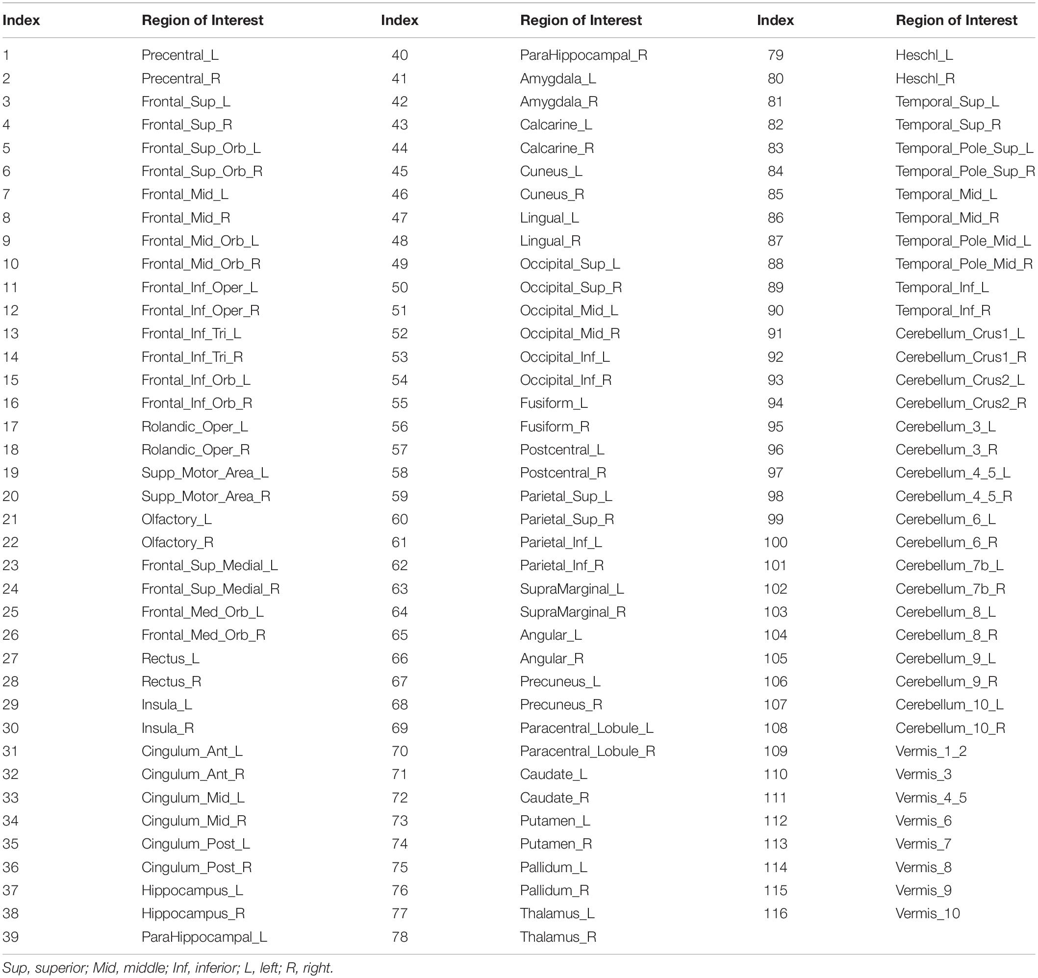
Table 1. List of regions of interest (ROIs) used when computing correlation matrices.
For comparison with the literature, we created an additional set of correlation matrices using the band-pass filtered data (at 0.01–0.08 Hz) for each subject. This is the frequency range typical of rs-fMRI analyses. Furthermore, to help explain the spectral makeup of this reference correlation matrix, we also generated correlation matrices using signals band-pass filtered into the frequency ranges corresponding to the IMFs. These were also averaged across subjects.
Statistical Comparisons
In this work, comparison between IMF clusters and tissue types is performed using the Student’s t-test, and linear correlation is used as the similarity index.
Results
The average results of the Monte Carlo simulation are shown in Figure 1. While the noiseless signal was successfully reconstructed using all three algorithms (not shown), they performed very differently when noise was introduced. It is evident that IMF1 derived using EMD (Figure 1B) contains two distinct modes that would ideally have been attributed to two different IMFs. This is the manifestation of modal spreading, which is also seen in the CEEMD results (Figure 1C). Due to the existence of substantial modal spreading, inter-modal mixing (overlapping between IMFs in the frequency domain) is also found. Compared to EMD and CEEMD, VMD was able to identify the 4 IMFs of the original simulated signal with the least mode spreading and mode mixing (Figure 1D), with the noise component being split across the 4 IMFs. These simulation results confirm the theory-based hypothesis of increased IMF-estimation precision using VMD.
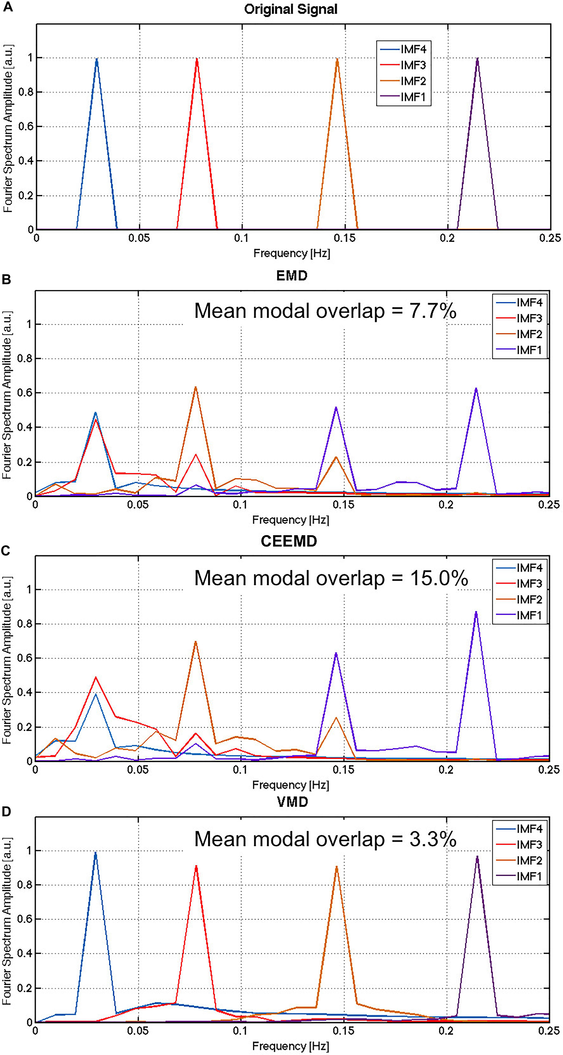
Figure 1. Comparison of performance for EMD, CEEMD and VMD on simulated data: The Fourier spectrum of the original noiseless signal (A) is compared to the average spectra obtained by EMD (B), CEEMD (C) and VMD (D) on the noisy version if the signal, averaged across all iterations of the Monte Carlo simulation. Gaussian noise was simulated in this case, with the SNR of the simulated noisy signals was approximately 1.2, approximated by the total power of the noise over the total power of the signal. In EMD and CEEMD, the 4 IMFs with highest powers are displayed.
Intrinsic Frequencies of the rs-fMRI Signal
Sample results from human rs-fMRI data are shown in Figure 2. VMD was able to extract IMFs from all data sets with high consistency and the lowest reconstruction error compared to both EMD and CEEMD. Based on results similar to these, IMFs were estimated for all voxels for each rs-fMRI data set. The corresponding IMF frequencies were organized into histograms for gray and white matter. A sample histogram of IMF frequencies is shown in Figure 3. Note that not all voxels returned 4 IMFs. Yet, when aggregated, the histograms revealed 4 clusters of IMF frequencies. This was common across all subjects, and across tissue types. Based on these clusters, IMF frequency ranges were identified for each subject in the group. We noted regional variability in the location of IMF clusters, with IMF4 being the most stable across brain regions and IMF2 being the least (Appendix Figure A3).
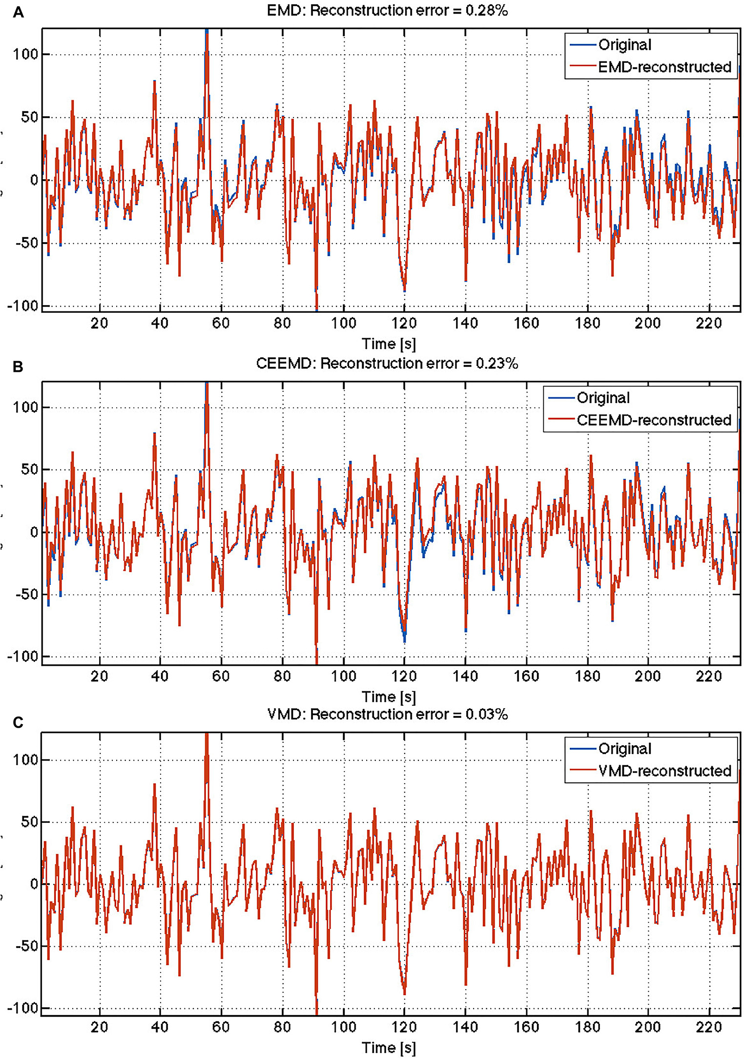
Figure 2. Comparison of reconstruction accuracy of rs-fMRI time series: The reconstruction errors are indicated for each algorithm: (A) EMD; (B) CEEMD; (C) VMD.
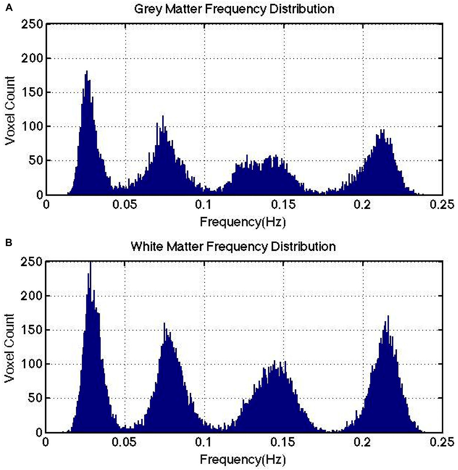
Figure 3. IMF frequency cluster distributions computed for a representative subject. Gray matter (A) and white matter (B) are shown to exhibit similar frequency clusters. Note that there is no direct link between the number of IMFs targeted for at the VMD stage and the number of IMF frequency clusters detected at the clustering stage.
The group-average VMD-decomposed peak frequencies in both gray and white matter are shown in Figure 4. Using the IMF-frequency clustering procedure described earlier, we identified 4 robust IMF-cluster frequency ranges. This was the case for all subjects and common to both gray and white matter. The frequency ranges of the 4 VMD IMF-frequency clusters are (mean frequency ± mean width/2):
• VMD IMF1: 0.20–0.24 Hz
• VMD IMF2: 0.13–0.17 Hz
• VMD IMF3: 0.063–0.098 Hz
• VMD IMF4: 0.021–0.036 Hz
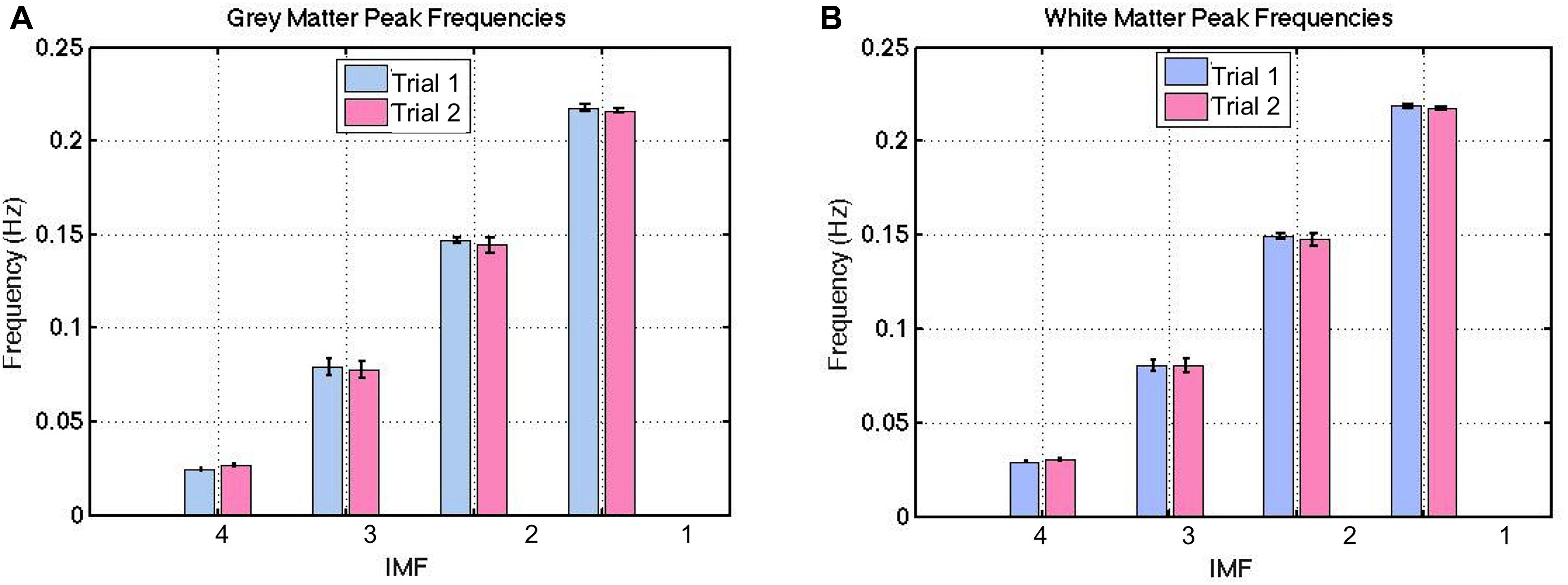
Figure 4. Between-session reproducibility of IMF frequency estimations. These frequencies were highly reproducible, with a ICC of 0.99 for both gray (A) and white matter (B). The error bars indicate the standard deviations across all subjects.
These frequencies were evenly distributed across the majority of voxels (both gray and white matter), with no specific spatial features. Thus, we do not show spatial maps of the frequency distributions. Also, these frequencies were highly reproducible based on the long-TR acquisitions (Figure 4), with an ICC of 0.99 for both gray and white matter. This was confirmed by the absence of significant difference between IMF peak frequencies across each trial in either tissue type (p > 0.21). Henceforth, all IMFs associated with actual rs-fMRI data will be identified by their cluster numbers (i.e., IMF1-4 refer to IMF cluster 1–4).
The IMF frequency clusters obtained from long-TR and short-TR data acquisitions are highly similar, as shown by the frequency groupings identified in Figures 5A,B – at a group level, there were no significant differences between the two TRs for any of the IMFs. However, the fractional IMF amplitudes are less consistent across different TRs, as shown in Figures 5C,D. In particular, IMF4 (the frequency cluster with the lowest mean frequency) is a consistently greater contributor to total spectral power in short-TR data sets. However, once again, the differences are not statistically significant.
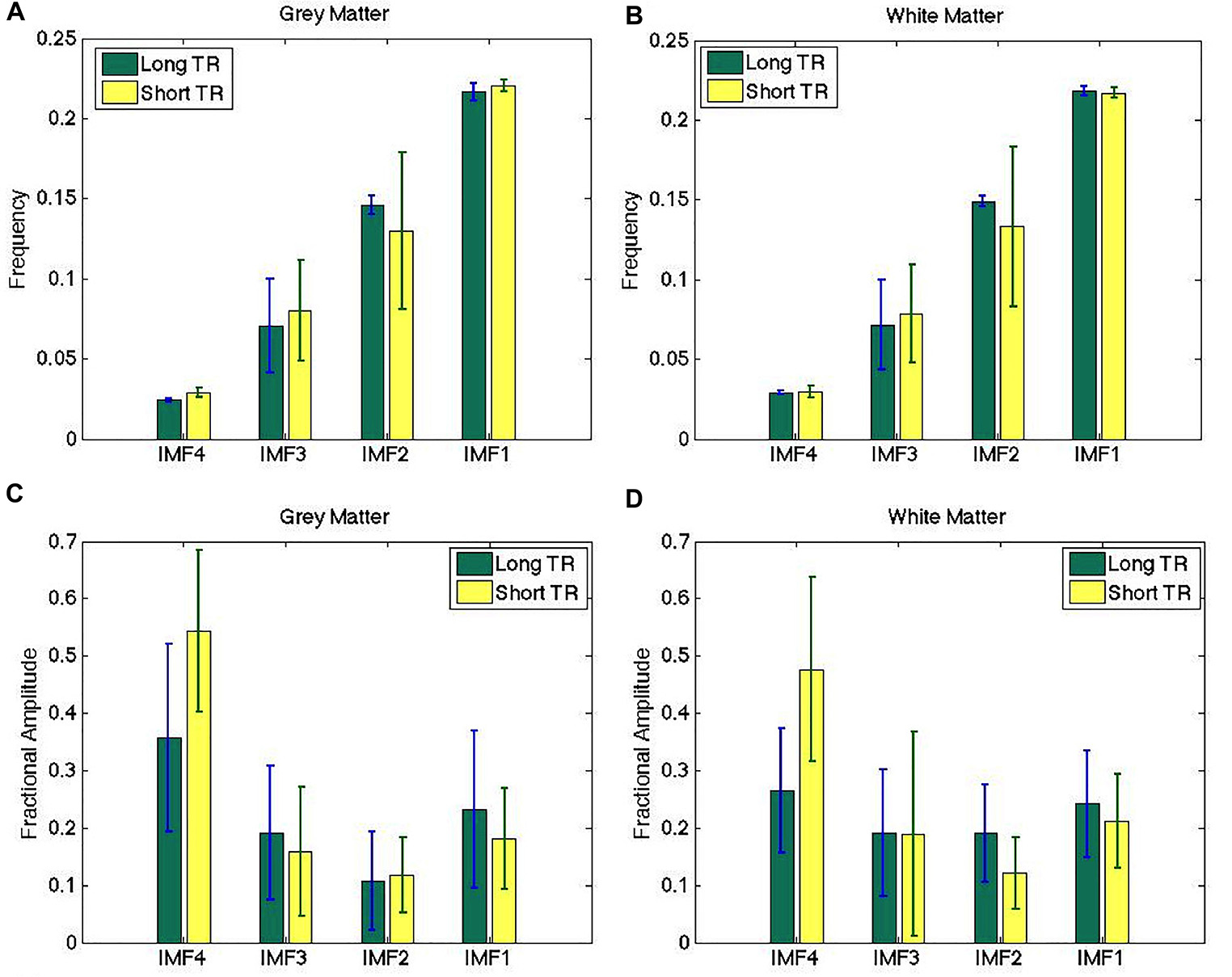
Figure 5. Comparison of IMF frequency (A,B) and fractional amplitude estimates (C,D) across different sampling rates. The IMF frequency groupings obtained from long-TR and short-TR data acquisitions are highly similar, although the fractional IMF amplitudes are less consistent across different TRs. There are no significant differences between the estimates obtained from the two data sets. The error bars indicate the standard deviations across all subjects.
In Figure 6, we show the spatial distribution of the fractional contributions of each VMD-derived IMF to the total spectral power of the rs-fMRI signal. The equivalent maps are shown for CEEMD-based IMFs as well. Note that for CEEMD as well, 4 IMF clusters were identified within the range of 0.01–0.25 Hz, confirming previous findings by Qian et al. (2015). However, due to the aforementioned decreasing spectral resolution with increasing IMF frequency exhibited by CEEMD, the frequency ranges of the CEEMD IMF clusters, listed below, are not directly comparable to those of VMD.
• CEEMD IMF1: 0.12–0.23 Hz
• CEEMD IMF2: 0.05–0.12 Hz
• CEEMD IMF3: 0.025–0.05 Hz
• CEEMD IMF4: 0.01–0.025 Hz
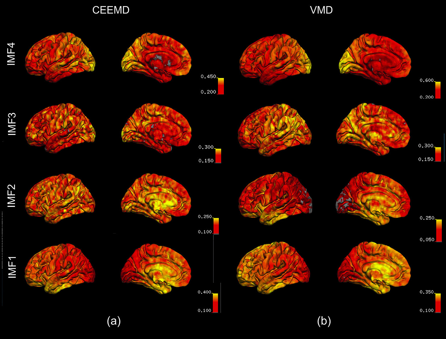
Figure 6. Spatial distribution of the fractional contributions of each IMF to the total spectral power of the rs-fMRI signal. The maps were averaged across all subjects for each IMF, and overlaid on a cortical surface. IMF4, which is associated with the lowest frequency, is markedly elevated in the occipital lobe, as reflected by VMD results (b). This is consistent with the CEEMD results (a). IMF1 and 2, associated with the highest frequencies, are elevated in the temporal lobe and the frontal/limbic cortices, respectively. These are not clearly seen in CEEMD-derived IMFs.
For both VMD and CEEMD results, maps of fractional spectral power were averaged across all subjects for each IMF, and overlaid on a cortical surface. IMF4, which is associated with the lowest frequency, is markedly elevated in the occipital lobe, as reflected by VMD results (Figure 6b). This is consistent with the CEEMD results (Figure 6a). IMF1 and 2, associated with the highest frequencies, were elevated in the temporal lobe and the frontal/limbic cortices, respectively. These are not clearly seen in CEEMD-derived IMFs. It is important to note that the CEEMD-derived IMF frequency ranges were as follows: IMF1: 0.12–0.23 Hz, IMF2: 0.05–0.10 Hz, IMF3: 0.025–0.05 Hz, IMF4: 0.01–0.025 Hz. These 4 IMF groupings were chosen to best match those of the VMD groupings.
Frequency Dependence of Network Organization
In Figure 7, we show strong RSN correlation patterns in areas that are part of the motor and control networks (indices 1–20), visual network (indices 43–60) and the medial-temporal network (indices 80–90). These results, based on the conventionally band-pass filtered rs-fMRI signal (to 0.01–0.08 Hz), are consistent with existing literature (Zhang and Li, 2014; Qian et al., 2015).
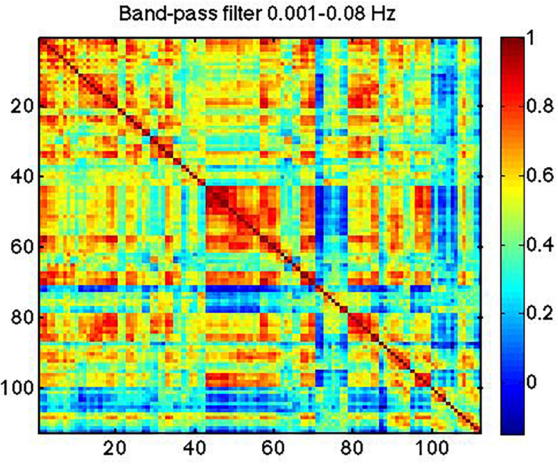
Figure 7. Typical correlation matrix based on the rs-fMRI signal within 0.001–0.08 Hz.
In Figure 8, we compare the RSN topology derived from VMD with those based on the 4 IMFs in comparable frequency ranges obtained using CEEMD. We can see that the highest correlations are found using IMF4, followed by IMF3, while no strong patterns were seen for IMFs 1 and 2. Moreover, IMFs 3 and 4 were associated with correlation matrices that most resemble that of the conventionally band-pass filtered signal (Figure 7), but not in IMF 1 and 2. Even in IMFs 3 and 4, the values of the correlations are much lower than those from band-pass filtering. However, the values are comparable to those obtained based on CEEMD. In fact, we note that the highest agreement between VMD and CEEMD results can be seen in IMF 4 (Figure 8B, r = 0.79), and secondarily in IMF 1 (Figure 8H, r = 0.58), the lowest and highest frequencies, respectively.
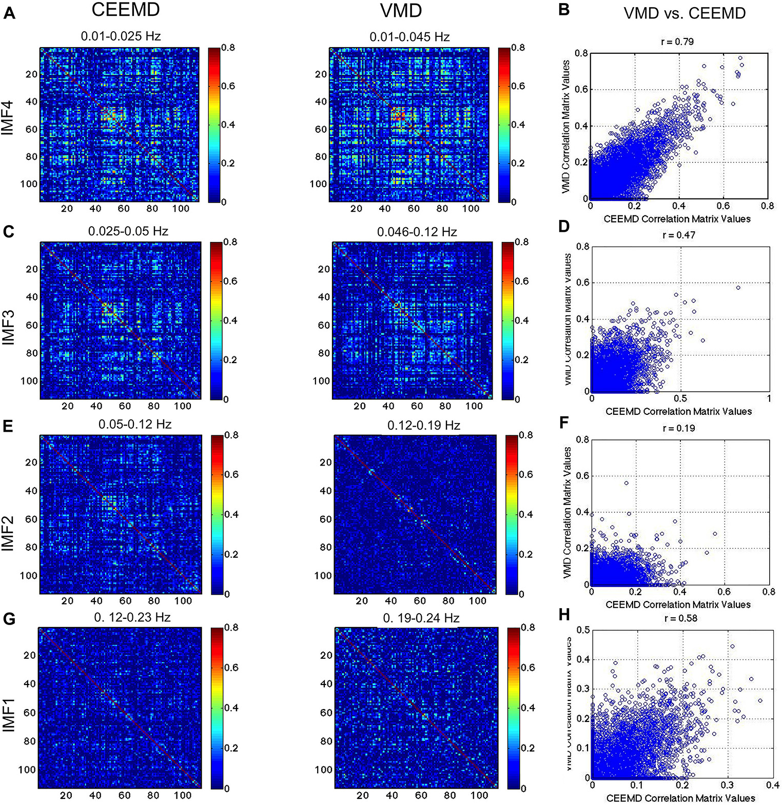
Figure 8. Comparison of VMD with CEEMD RSN-matrix topology. IMFs 4, 3, 2, and 1 are represented in (A), (B), (C), and (D), respectively. The VMD and CEEMD IMFs are in comparable frequency ranges. The highest agreement between VMD and CEEMD results are seen in IMF 4 (r = 0.79), and secondarily in IMF 1 (r = 0.58), the lowest and highest frequencies, respectively. Note that the maximum displayed correlations value has been reduced from 1 to 0.8 for display purposes.
In Figure 9, we repeat the comparison, substituting CEEMD with band-pass filtered versions of the rs-fMRI data, with each band-pass filter range determined based on VMD derivations of IMF frequency ranges. The conventional RSN topology can be observed across all band-passed frequencies (the top-left, middle and bottom-right areas of the matrix corresponding to the sensorimotor, visual and default-mode network, respectively), although it is most prominent at the lowest frequency. While this trend of decreasing correlation with increasing frequency is consistent with findings from VMD, the strengths of the correlations in VMD are markedly lower than those found using band-pass filtering. We also notice that the similarities (Figures 9B,D,F,H) are lower than observed between VMD and CEEMD results.
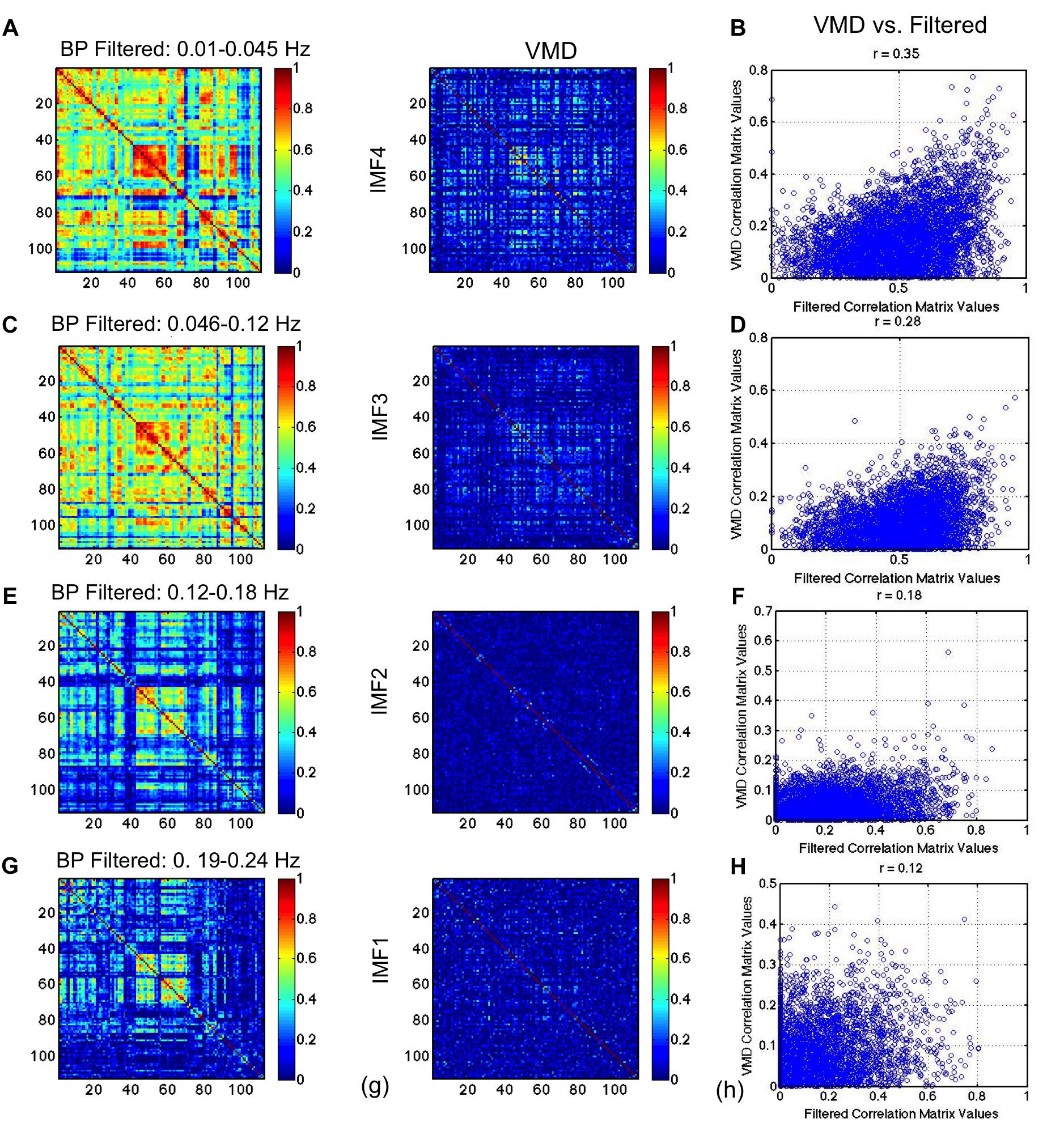
Figure 9. Comparison of VMD RSN-matrix topology with results of band-pass filtering. IMFs 4, 3, 2, and 1 are represented in (A), (B), (C), and (D), respectively. Each band-pass filter range determined based on VMD derivations of IMF frequency ranges. The conventional RSN topology can be observed across all band-passed frequencies, although it is most prominent at the lowest frequency. While this trend of decreasing correlation with increasing frequency is consistent with findings from VMD, the strengths of the correlations in VMD are markedly lower than those found using band-pass filtering.
Discussion
In studying the spectral properties of the rs-fMRI signal, there is an increasing desire to use data-driven methods rather than band-pass filtering to decipher frequency content (Niazy et al., 2011; Qian et al., 2015). The main differences between methods based intrinsic-modal decomposition and those based on band-pass filtering are: (1) results and interpretations of band-pass filtering are sensitive to the shape of the band-pass filter; (2) band-pass filtering is sensitive to non-linearity in the signal, such as introduced when the signal is non-stationary. The latter is particularly the case in rs-fMRI, affecting the oscillatory validity of band-pass filtered rs-fMRI signal components.
Our work is novel in the following aspects: (1) instead of relying on the assumption that our data-driven method accurately decomposes the modes of the signal, we test this accuracy using rs-fMRI-informed simulations; (2) we not only compared the findings from short-TR acquisitions with those based on conventional acquisitions (TR = 2 s), but also assessed the reproducibility of these results for both scenarios; (3) instead of defining the rs-fMRI spectral information by broad frequency ranges (up to >1 Hz), we specifically target the frequency range typically used in functional-connectivity analyses (<0.25 Hz).
Our primary findings are: (1) the rs-fMRI signal within the 0.01–0.25 Hz range can be consistently characterized by four intrinsic modal clusters (frequency clusters), centered at 0.028, 0.080, 0.15, and 0.22 Hz, respectively; (2) these frequency clusters were highly reproducible, and independent of rs-fMRI data sampling rate; (3) not all frequencies were associated with equivalent RSN topology, in contrast to previous findings.
Intrinsic Frequencies of the rs-fMRI Signal
In this work, we demonstrate that as expected, compared to the previously used EMD and CEEMD techniques, VMD resulted in less inter-modal mixing as well as minimal modal spreading (Figure 1). When applied to rs-fMRI data, we demonstrate high reconstruction accuracy when using VMD-derived IMFs relative to the alternatives (EMD and CEEMD). We also see that VMD is able to decompose fMRI signals in a reproducible manner, given the small variability associated with each IMF frequency across 8 subjects. Interestingly, we found that both gray and white matter of the healthy brain are characterized by IMF clusters centered at the frequencies of 0.028, 0.080, 0.15, and 0.23 Hz, identifiable in all of our subjects. While all brain voxels exhibited these frequencies, the contribution of each to the total signal power varied spatially (Figure 6). In the literature, a similar clustering of IMF frequencies across brain voxels has been observed previously using EMD (Song et al., 2014) and CEEMD (Qian et al., 2015), although the previously reported center frequencies were 0.02, 0.04, 0.08, and 0.17 Hz, respectively. This difference is likely driven by the higher degree of mode spreading in the higher-frequency IMFs that is inherent in CEEMD, as described in the sections “Introduction” and “Results.”
When we used short-TR acquisitions (TR on the scale of 300 ms) (Niazy et al., 2011; Kalcher et al., 2014) to reduce respiratory and cardiac aliasing in the frequency range of interest, our findings of these IMF cluster frequencies did not change. Moreover, we acquired two trials of rs-fMRI data per subject, within the same scan session. To our best knowledge, no previous study has examined the reproducibility of intrinsic mode functions derived from rs-fMRI data, nor did any study examine the TR sensitivity of the decompositions. The frequency clusters we identified were highly reproducible across fMRI trials, and insensitive to the TR used (Figure 5), strengthening our confidence in the potential biological relevance of our findings.
Possible Interpretations of Intrinsic rs-fMRI Frequencies
Our current data do not permit us to conclusively pinpoint the physiological source(s) of these frequencies, although we may refer to independent evidence of physiological oscillatory signatures.
IMF4, being at the lowest frequency, contributed the most to the overall signal power. This is in general agreement with findings by Kalcher et al. (2014), who nonetheless examined a different set of frequency bands (i.e., < 0.1 Hz, 0.1–0.25 Hz, 0.25–0.75 Hz, and 0.75–1.4 Hz). It has been well established that within the 0.01–0.25 Hz frequency range, low-frequency cardiac-rate variations and respiratory-volume variations are observable near 0.01 Hz and 0.036 Hz in fMRI data, respectively. Therefore, it is probable that IMF4 (range: 0.021–0.031 Hz) is associated with these phenomena. Indeed, the high power contribution of IMF4 to the occipital region (Figure 6) is consistent with previous reports on the amplitude of rs-fMRI BOLD signal modulation by respiratory variability (Chang and Glover, 2009a; Tong et al., 2011; Golestani et al., 2015). Moreover, the contribution of IMF4 to the overall power is the only fraction that is lower in white matter than in gray matter (Figures 5C,D), in agreement with recent findings by Tong et al. (2016), although the difference is not statistically significant. However, the effects of these different physiological variances could not be distinguished from one another, potentially due to oscillatory variations across different tissue locations (Chang and Glover, 2009a; Golestani et al., 2015). Moreover, while we may expect the short-TR data to exhibit lower IMF4 amplitude than long-TR data due to the enhanced ability for physiological nose removal, it is unclear which IMF the physiological signal would be aliased into in the long-TR data. At the maximum sampling frequency of 0.25 Hz, such noise sources could equally alias into IMF3. Indeed, such is the case in the gray matter, albeit the difference between short- and long-TR not statistically significant.
The frequency ranges of IMF3 (0.063–0.098 Hz, peaking at 0.080 Hz) and IMF2 (0.13–0.17 Hz, peaking at 0.15 Hz) have both been associated with low-frequency vascular oscillations (Tong and Frederick, 2014; Hocke et al., 2016; Tong et al., 2016). A major source of these vascular oscillations is vasomotion (Intaglietta, 1990; Rivadulla et al., 2011). Vasomotion has long been observed in the BOLD signal (Kiviniemi et al., 2000; Cordes et al., 2001), and refers to a spontaneous oscillation in the diameter of primarily pre-capillary vessels (Cooper et al., 1966) that propagates through the entire vasculature but does not influence cognitive processes. Vasomotion is associated with oscillations in red blood-cell velocity (Biswal and Hudetz, 1996) and modulates local blood flow (Morita et al., 1994; Biswal and Hudetz, 1996; Aalkjaer et al., 2011). In particular, initially observed in superficial blood vessels at around 0.1 Hz (Mayhew et al., 1996; Meyer et al., 2003; Murphy et al., 2013), vasomotion’s main frequency signature has been consistent between the animal (Mayhew et al., 1996; Bernardi, 1997; Haddock et al., 2002; Meyer et al., 2003) and human subcutaneous endothelium (Kvernmo et al., 1999, 1998).
The origins of vasomotion observed in fMRI could be caused by oscillations in both vascular diameter (Intaglietta, 1990; Biswal and Hudetz, 1996) and blood oxygenation (Biswal and Hudetz, 1996; Nikulin et al., 2014). Until recently, there have not been fMRI-based measurements of vasomotion in the human brain. Rayshubskiy et al. (2014) were able to measure sinusoids at (∼0.1 Hz near using intraoperative optical intrinsic-signal imaging and preoperative fMRI near the same pial veins of awake humans. However, an added challenge of in vivo isolation of vasomotion is that vasomotion frequency may in fact be dependent on vascular size, increasing with decrease vessel size (Intaglietta, 1990; Harrison and Cai, 2003). This, coupled with the fact that frequencies below 0.1 Hz (clusters IMF3 and IMF4) have typically revealed robust brain-network patterns, suggests that the effects of vasomotion may be embodied in IMF2. In support of the closer neuronal relevance of IMF3, we note that the regions of the highest fractional power distribution by IMF3 are the superior parietal, posterior cingulate and precuneus regions (Figure 6), coinciding with regions of high resting neuronal activity determined using positron-emission tomography (Raichle, 2011).
At very high frequencies (IMF1), the fractional spectral power is second only to the contribution of IMF4 (very low frequencies), as shown in Figure 5. This frequency band (0.20–0.24 Hz, peaking at 0.21 Hz) has previously been associated with head motion (Razavi et al., 2008). Although motion was corrected in the preprocessing pipeline, the effect of motion cannot be completely removed (Faraji-Dana et al., 2016a, b). In the case of the long-TR data, this frequency may also be associated with aliased cardiac pulsations, although this theory is refuted by the fact that IMF1 is equally strong in short-TR and long-TR data sets. The functional significance of IMF1 will need to be interpreted in the context of network-related features.
Frequency Dependence of Network Organization
We found that the functional connectivity patterns of RSNs are dependent on frequency and that not all IMFs reveal the same connectivity patterns, contrary to previous reports (Niazy et al., 2011; Qian et al., 2015). The connectivity-matrix patterns found in IMF 3 and 4 (Figure 7) were most similar to those from the 0.01–0.08 Hz band-passed signal (Figure 8), and were not seen in the higher frequency range (IMF 1 and 2). This is expected and is likely to reflect differences in biological significance of high- and low-frequency signals as described earlier.
Our findings echo those of Song et al. (2014), who found cortical RSNs to be best represented in low-frequency oscillations (<0.05 Hz). While both IMF clusters 3 and 4 demonstrated visible RSN connectivity-matrix patterns (Figures 8A,B), IMF4 was associated with the highest signal power and highest correlation. The fact that IMF4 is also most likely to contain low-frequency physiological contributions supports previous findings that physiological processes are stable (Birn, 2012) and can equally generate highly robust connectivity-matrix patterns (Chang and Glover, 2009b). This is an important point to consider in interpreting the quality of RSN results based on strength and reproducibility alone.
However, our findings contrast previous findings that RSNs are a broadband phenomenon (Niazy et al., 2011; Qian et al., 2015). These previous findings are in line with band-pass filtering results (Figure 9), whereby similar connectivity patterns are observed across all frequency bands. Nonetheless, previous work has also demonstrated the frequency dependence of task-fMRI-based brain networks (Baria et al., 2011). Moreover, our results are also corroborated by near-infrared optical connectivity measures in the resting state (Sasai et al., 2011), whereby long-range and local connections were associated with distinct frequencies within the 0.009–0.1 Hz range.
As, we demonstrated significant mode mixing using EMD and CEEMD (Figure 1), we argue this effect could have resulted in the similarities between IMFs that were previously reported. The same logic may explain why band-pass filtered maps were similar across frequency bands, as IMFs are difficult to isolate using such filtering methods. Notwithstanding, the similarity of the IMF1 connectivity matrices obtained through VMD and CEEMD (Figure 8A) despite their different frequency bands, serves to cross validate previous findings against our findings at low frequencies. Lastly, we are unclear as to the reason the correlations values corresponding to VMD are much lower than those based on band-pass filtering (Figure 9).
On average (across the group), the functional connectivity values found with the VMD and CEEMD are lower than found with conventional bandpass filtering. This is to be expected, signal bands produced by BPF always have the same frequency ranges, but IMFs do not always have the same frequency ranges, and can vary from subject to subject in that regard. This variability can reflect in inter-subject variations in connectivity strength, as exemplified in the Appendix Figure A4.
Limitations
In this work, we focused on the use of the empirical model decomposition (EMD) family of methods, and more specifically, on the use of the VMD method to provide estimates of intrinsic modes while avoiding mode mixing. In general, EMD has long been used for investigating the frequency composition of biological signals that are non-stationary. Compared to prevalent techniques such as independent-component analysis (ICA), EMD has the advantage of being able to operate on individual signals instead relying on multiple measurements. Furthermore, the focus on EMD is “intrinsic frequencies” instead of statistical independence, more directly addressing our main focus. Nevertheless, a combination of EMD and ICA may be investigated in our future work.
In adopting VMD, the main thrust of our work is to reduce the spectral overlapping in previous works. Our choice of IMFs is driven by precision and reproducibility, which may be a strength and a limitation, depending on whether the intrinsic modes are expected to be reproducible. Such assumptions have been used broadly in the rs-fMRI field, but requires further dissection. While the motivation for using VMD (and EMD in general) is the non-stationarity of the rs-fMRI signal, the ground-truth testing was done using simulated stationary signals. As it was unclear what alternative noise model would be appropriate for such a simulation (where the ground truth signal vs. noise distributions are unknown in rs-fMRI data), we used white noise. While this may be a limitation, such an approach provided us with a clear way to evaluate the techniques – if a given technique could not faithfully reconstruct a stationary signal, its performance on a non-stationary signal could be no better than presented. Although we have identified the frequency cluster IMF3 as most representative of neutrally relevant BOLD, both by frequency and by spatial contribution, we are not able, in the current study, to provide direct experimental verification. Likewise, we are unable to determine the amount of physiological contributions to IMF4, which is deemed most representative of respiratory and cardiac effects using the current data. In future studies, we will involve physiological monitoring during the rs-fMRI sessions. This will be augmented by the use of simultaneous EEG-fMRI to capture neural fluctuations as well as blood-oxygenation effects, ideally in the presence of stimuli that can modulate baseline cerebral metabolism. Furthermore, the use phase locking is also an effective tool for estimating the sources of the IMFs and their interplay (Pfurtscheller et al., 2017), given sufficient SNR.
Furthermore, while we determined that the cluster IMF2 is most likely associated with low-frequency vascular oscillations (or vasomotion), the central frequency of IMF2 is 0.15 Hz, deviating from the typically reported to be 0.1 Hz in surface vessels. Furthermore, we did not find any observable vascular networks based on specific frequencies in the fMRI signal. While we have evidence to believe the frequency of vasomotion increases with decreasing diameter (Intaglietta, 1990), our ability to isolate smaller blood vessels is limited by the spatial resolution of the fMRI acquisition and by the BOLD effect itself. One possibility for targeting this issue is to repeat these measurements in conjunction with independent monitoring of subcutaneous vasomotion as well as vascular stimuli that can modulate vasomotion amplitude.
Finally, in this study, we do not examine network properties such as the differences between local and long-range connections in our study of RSN frequency dependence. The intention of our current work is to establish the validity of our decomposition procedure, and a comprehensive examination of the frequency dependence of multiple network metrics will be part of our future work.
Data Availability
The datasets generated for this study are available on request to the corresponding author.
Ethics Statement
This study was approved by the Baycrest Research Ethics Board. All subjects provided informed written consent.
Author Contributions
NY contributed to 90% of the analysis and 30% of the writing. NO contributed to 10% of the analysis. JC contributed to 70% of the analysis and writing.
Funding
This research was supported by the Natural Sciences and Engineering Council of Canada (NSERC FGPIN# 418443 to JC and NSERC Undergraduate Research Awards to NY and NO), the Canadian Institutes of Health Research (CIHR: FRN# 126164 to JC), and the Sandra Rotman Foundation.
Conflict of Interest Statement
The authors declare that the research was conducted in the absence of any commercial or financial relationships that could be construed as a potential conflict of interest.
Acknowledgments
We thank Prof. Stephen Smith (Oxford) for helpful discussions on the manuscript.
Supplementary Material
The Supplementary Material for this article can be found online at: https://www.frontiersin.org/articles/10.3389/fnins.2019.00900/full#supplementary-material
Footnotes
References
Aalkjaer, C., Boedtkjer, D., and Matchkov, V. (2011). Vasomotion - what is currently thought? Acta Physiol. 202, 253–269. doi: 10.1111/j.1748-1716.2011.02320.x
Baria, A. T., Baliki, M. N., Parrish, T., and Apkarian, A. V. (2011). Anatomical and functional assemblies of brain bold oscillations. J. Neurosci. 31, 7910–7919. doi: 10.1523/JNEUROSCI.1296-11.2011
Bernardi, L. (1997). Reduction of 0.1 Hz microcirculatory fluctuations as evidence of sympathetic dysfunction in insulin-dependent diabetes. Cardiovasc. Res. 34, 185–191. doi: 10.1016/s0008-6363(97)00017-5
Birn, R. M. (2012). The role of physiological noise in resting-state functional connectivity. Neuroimage 62, 864–870. doi: 10.1016/j.neuroimage.2012.01.016
Birn, R. M., Smith, M. A., Jones, T. B., and Bandettini, P. A. (2008). The respiration response function: the temporal dynamics of fMRI signal fluctuations related to changes in respiration. Neuroimage 40, 644–654. doi: 10.1016/j.neuroimage.2007.11.059
Biswal, B. B., and Hudetz, A. G. (1996). Synchronous oscillations in cerebrocortical capillary red blood cell velocity after nitric oxide synthase inhibition. Microvasc. Res. 52, 1–12. doi: 10.1006/mvre.1996.0039
Chang, C., and Glover, G. H. (2009a). Effects of model-based physiological noise correction on default mode network anti-correlations and correlations. Neuroimage 47, 1448–1459. doi: 10.1016/j.neuroimage.2009.05.012
Chang, C., and Glover, G. H. (2009b). Relationship between respiration, end-tidal CO2, and bold signals in resting-state fMRI. Neuroimage 47, 1381–1393. doi: 10.1016/j.neuroimage.2009.04.048
Cooper, R., Crow, H. J., Walter, W. G., and Winter, A. L. (1966). Regional control of cerebral vascular reactivity and oxygen supply in man. Brain Res. 3, 174–191. doi: 10.1016/0006-8993(66)90075-8
Cordes, D., Haughton, V. M., Arfanakis, K., Carew, J. D., Turski, P. A., Moritz, C. H., et al. (2001). Frequencies contributing to functional connectivity in the cerebral cortex in “resting-state” data. AJNR Am. J. Neuroradiol. 22, 1326–1333.
Dragomiretskiy, K., and Zosso, D. (2014). Variational mode decomposition. IEEE Trans. Signal Process. 62, 531–544.
Faraji-Dana, Z., Tam, F., Chen, J. J., and Graham, S. J. (2016a). A robust method for suppressing motion-induced coil sensitivity variations during prospective correction of head motion in fMRI. Magn. Reson. Imaging 34, 1206–1219. doi: 10.1016/j.mri.2016.06.005
Faraji-Dana, Z., Tam, F., Chen, J. J., and Graham, S. J. (2016b). Interactions between head motion and coil sensitivity in accelerated fMRI. J. Neurosci. Methods 270, 46–60. doi: 10.1016/j.jneumeth.2016.06.005
Feinberg, D. A., Moeller, S., Smith, S. M., Auerbach, E., Ramanna, S., Glasser, M. F., et al. (2010). Multiplexed echo planar imaging for sub-second whole brain fMRI and fast diffusion imaging. PLoS One 5:e15710. doi: 10.1371/journal.pone.0015710
Fischl, B., and Dale, A. M. (2000). Measuring the thickness of the human cerebral cortex from magnetic resonance images. Proc. Natl. Acad. Sci. U.S.A. 97, 11050–11055. doi: 10.1073/pnas.200033797
Fischl, B., Sereno, M. I., Tootell, R. B., and Dale, A. M. (1999). High-resolution intersubject averaging and a coordinate system for the cortical surface. Hum. Brain Mapp. 8, 272–284. doi: 10.1002/(sici)1097-0193(1999)8:4<272::aid-hbm10>3.0.co;2-4
Fischl, B., van der Kouwe, A., Destrieux, C., Halgren, E., Segonne, F., Salat, D. H., et al. (2004). Automatically parcellating the human cerebral cortex. Cereb. Cortex 14, 11–22. doi: 10.1093/cercor/bhg087
Golestani, A. M., Chang, C., Kwinta, J. B., Khatamian, Y. B., and Chen, J. J. (2015). Mapping the end-tidal CO2 response function in the resting-state BOLD fMRI signal: spatial specificity, test–retest reliability and effect of fMRI sampling rate. Neuroimage 104, 266–277. doi: 10.1016/j.neuroimage.2014.10.031
Haddock, R. E., Hirst, G. D. S., and Hill, C. E. (2002). Voltage independence of vasomotion in isolated irideal arterioles of the rat. J. Physiol. 540, 219–229. doi: 10.1113/jphysiol.2001.013698
Harrison, D. G., and Cai, H. (2003). Endothelial control of vasomotion and nitric oxide production. Cardiol. Clin. 21, 289–302. doi: 10.1016/s0733-8651(03)00073-0
Hocke, L. M., Tong, Y., Lindsey, K. P., de, B., and Frederick, B. (2016). Comparison of peripheral near-infrared spectroscopy low-frequency oscillations to other denoising methods in resting state functional MRI with ultrahigh temporal resolution. Magn. Reson. Med. 76, 1697–1707. doi: 10.1002/mrm.26038
Huang, N. E., Shen, Z., Long, S. R., Wu, M. C., Shih, H. H., Zheng, Q., et al. (1998). The empirical mode decomposition and the hilbert spectrum for nonlinear and non-stationary time series analysis. Proc. R. Soc. Lond. A Math. Phys. Sci. 454, 903–905.
Intaglietta, M. (1990). Vasomotion and flowmotion: physiological mechanisms and clinical evidence. Vasc. Med. 1, 101–112. doi: 10.1177/1358836x9000100202
Jenkinson, M., Bannister, P., Brady, M., and Smith, S. (2002). Improved optimization for the robust and accurate linear registration and motion correction of brain images. Neuroimage 17, 825–841. doi: 10.1006/nimg.2002.1132
Jenkinson, M., and Smith, S. (2001). A global optimisation method for robust affine registration of brain images. Med. Image Anal. 5, 143–156. doi: 10.1016/S1361-8415(01)00036-6
Kalcher, K., Boubela, R. N., Huf, W., Bartova, L., Kronnerwetter, C., Derntl, B., et al. (2014). The spectral diversity of resting-state fluctuations in the human brain. PLoS One 9:e93375. doi: 10.1371/journal.pone.0093375
Kiviniemi, V., Jauhiainen, J., Tervonen, O., Paakko, E., Oikarinen, J., Vainionpaa, V., et al. (2000). Slow vasomotor fluctuation in fMRI of anesthetized child brain. Magn. Reson. Med. 44, 373–378. doi: 10.1002/1522-2594(200009)44:3<373::aid-mrm5>3.3.co;2-g
Kvernmo, H. D., Stefanovska, A., Bracic, M., Kirkeboen, K. A., and Kvernebo, K. (1998). Spectral analysis of the laser doppler perfusion signal in human skin before and after exercise. Microvasc. Res. 56, 173–182. doi: 10.1006/mvre.1998.2108
Kvernmo, H. D., Stefanovska, A., Kirkeboen, K. A., and Kvernebo, K. (1999). Oscillations in the human cutaneous blood perfusion signal modified by endothelium-dependent and endothelium-independent vasodilators. Microvasc. Res. 57, 298–309. doi: 10.1006/mvre.1998.2139
Lahmiri, S. (2014). Comparative study of ECG signal denoising by wavelet thresholding in empirical and variational mode decomposition domains. Healthc. Technol. Lett. 1, 104–109. doi: 10.1049/htl.2014.0073
Liu, W., Cao, S., and Chen, Y. (2016). Applications of variational mode decomposition in seismic time-frequency analysis. Geophysics 81, V365–V378.
Mark, C. I., Mazerolle, E. L., and Chen, J. J. (2015). Metabolic and vascular origins of the BOLD effect: implications for imaging pathology and resting-state brain function. J. Magn. Reson. Imaging 42, 231–246. doi: 10.1002/jmri.24786
Mayhew, J. E., Askew, S., Zheng, Y., Porrill, J., Westby, G. W., Redgrave, P., et al. (1996). Cerebral vasomotion: a 0.1-Hz fluctuation in reflected light imaging of neural activity. Neuroimage 4, 183–193. doi: 10.1006/nimg.1996.0069
Mert, A. (2016). ECG feature extraction based on the bandwidth properties of variational mode decomposition. Physiol. Meas. 37, 530–543. doi: 10.1088/0967-3334/37/4/530
Meyer, M. F., Rose, C. J., Hülsmann, J. O., Schatz, H., and Pfohl, M. (2003). Impaired 0.1-Hz vasomotion assessed by laser doppler anemometry as an early index of peripheral sympathetic neuropathy in diabetes. Microvasc. Res. 65, 88–95. doi: 10.1016/s0026-2862(02)00015-8
Morita, Y., Hardebo, J. E., and Bouskela, E. (1994). Influence of cerebrovascular parasympathetic nerves on resting cerebral blood flow, spontaneous vasomotion, autoregulation, hypercapnic vasodilation and sympathetic vasoconstriction. J. Auton. Nerv. Syst. 49, S9–S14.
Murphy, K., Birn, R. M., and Bandettini, P. A. (2013). Resting-state fMRI confounds and cleanup. Neuroimage 80, 349–359. doi: 10.1016/j.neuroimage.2013.04.001
Niazy, R. K., Xie, J., Miller, K., Beckmann, C. F., and Smith, S. M. (2011). Spectral characteristics of resting state networks. Brain Res. 193, 259–276. doi: 10.1016/b978-0-444-53839-0.00017-x
Nikolaou, F., Orphanidou, C., Papakyriakou, P., Murphy, K., Wise, R. G., and Mitsis, G. D. (2016). Spontaneous physiological variability modulates dynamic functional connectivity in resting-state functional magnetic resonance imaging. Philos. Trans. A Math. Phys. Eng. Sci. 374:20150183. doi: 10.1098/rsta.2015.0183
Nikulin, V. V., Fedele, T., Mehnert, J., Lipp, A., Noack, C., Steinbrink, J., et al. (2014). Monochromatic ultra-slow (~0.1Hz) oscillations in the human electroencephalogram and their relation to hemodynamics. Neuroimage 97, 71–80. doi: 10.1016/j.neuroimage.2014.04.008
Pfurtscheller, G., Schwerdtfeger, A., Brunner, C., Aigner, C., Fink, D., Brito, J., et al. (2017). Distinction between neural and vascular bold oscillations and intertwined heart rate oscillations at 0.1 Hz in the resting state and during movement. PLoS One 12:e0168097. doi: 10.1371/journal.pone.0168097
Qian, L., Zhang, Y., Zheng, L., Shang, Y., Gao, J.-H., and Liu, Y. (2015). Frequency dependent topological patterns of resting-state brain networks. PLoS One 10:e0124681. doi: 10.1371/journal.pone.0124681
Rayshubskiy, A., Wojtasiewicz, T. J., Mikell, C. B., Bouchard, M. B., Timerman, D., Youngerman, B. E., et al. (2014). Direct, intraoperative observation of ~0.1 Hz hemodynamic oscillations in awake human cortex: implications for fMRI. Neuroimage 87, 323–331. doi: 10.1016/j.neuroimage.2013.10.044
Razavi, M., Eaton, B., Paradiso, S., Mina, M., Hudetz, A. G., and Bolinger, L. (2008). Source of low-frequency fluctuations in functional MRI signal. J. Magn. Reson. Imaging 27, 891–897. doi: 10.1002/jmri.21283
Rivadulla, C., Labra, D. C., Grieve, L. K., and Cudeiro, J. (2011). Vasomotion and neurovascular coupling in the visual thalamus in vivo. PLoS One 6:e28746. doi: 10.1371/journal.pone.0028746
Salvador, R., Suckling, J., Schwarzbauer, C., and Bullmore, E. (2005). Undirected graphs of frequency-dependent functional connectivity in whole brain networks. Philos. Trans. R Soc. Lond. B Biol. Sci. 360, 937–946. doi: 10.1098/rstb.2005.1645
Sasai, S., Homae, F., Watanabe, H., and Taga, G. (2011). Frequency-specific functional connectivity in the brain during resting state revealed by NIRS. Neuroimage 56, 252–257. doi: 10.1016/j.neuroimage.2010.12.075
Segonne, F., Dale, A. M., Busa, E., Glessner, M., Salat, D., Hahn, H. K., et al. (2004). A hybrid approach to the skull stripping problem in MRI. Neuroimage 22, 1060–1075. doi: 10.1016/j.neuroimage.2004.03.032
Segonne, F., Pacheco, J., and Fischl, B. (2007). Geometrically accurate topology-correction of cortical surfaces using nonseparating loops. IEEE Trans. Med. Imaging 26, 518–529. doi: 10.1109/TMI.2006.887364
Sled, J. G., Zijdenbos, A. P., and Evans, A. C. (1998). A non-parametric method for automatic correction of intensity non-uniformity in MRI data. IEEE Trans. Med. Imaging 17, 87–97. doi: 10.1109/42.668698
Song, X., Zhang, Y., and Liu, Y. (2014). Frequency specificity of regional homogeneity in the resting-state human brain. PLoS One 9:e86818. doi: 10.1371/journal.pone.0086818
Tong, Y., and Frederick, B. D. (2014). Studying the spatial distribution of physiological effects on bold signals using ultrafast fMRI. Front. Hum. Neurosci. 8:196. doi: 10.3389/fnhum.2014.00196
Tong, Y., Hocke, L. M., Lindsey, K. P., Erdoğan, S. B., Vitaliano, G., Caine, C. E., et al. (2016). Systemic low-frequency oscillations in bold signal vary with tissue type. Front. Neurosci. 10:313. doi: 10.3389/fnins.2016.00313
Tong, Y., Lindsey, K. P., and De, B. F. B. (2011). Partitioning of physiological noise signals in the brain with concurrent near-infrared spectroscopy and fMRI. J. Cereb. Blood Flow Metab. 31, 2352–2362. doi: 10.1038/jcbfm.2011.100
Tripathy, R. K., Sharma, L. N., and Dandapat, S. (2016). Detection of shockable ventricular arrhythmia using variational mode decomposition. J. Med. Syst. 40:79. doi: 10.1007/s10916-016-0441-5
Tzourio-Mazoyer, N., Landeau, B., Papathanassiou, D., Crivello, F., Etard, O., Delcroix, N., et al. (2002). Automated anatomical labeling of activations in SPM using a macroscopic anatomical parcellation of the MNI MRI single-subject brain. Neuroimage 15, 273–289. doi: 10.1006/nimg.2001.0978
Wu, Z., and Huang, N. E. (2009). Ensemble empirical mode decomposition: a noise-assisted data analysis method. Adv. Adapt. Data Anal. 01, 1–41. doi: 10.1142/s1793536909000047
Xiao, Q., Li, J., Bai, Z., Sun, J., Zhou, N., and Zeng, Z. (2016). A small leak detection method based on VMD adaptive de-noising and ambiguity correlation classification intended for natural gas pipelines. Sensors 16:2116. doi: 10.3390/s16122116
Yeh, J.-R., Lin, T.-Y., Chen, Y., Sun, W.-Z., Abbod, M. F., and Shieh, J.-S. (2012). Investigating properties of the cardiovascular system using innovative analysis algorithms based on ensemble empirical mode decomposition. Comput. Math. Methods Med. 2012:943431. doi: 10.1155/2012/943431
Zhang, S., and Li, C. (2014). Functional clustering of the human inferior parietal lobule by whole-brain connectivity mapping of resting-state functional magnetic resonance imaging signals. Brain Connect. 4, 53–69. doi: 10.1089/brain.2013.0191
Zhang, Y., Brady, M., and Smith, S. (2001). Segmentation of brain MR images through a hidden Markov random field model and the expectation-maximization algorithm. IEEE Trans. Med. Imaging 20, 45–57. doi: 10.1109/42.906424
Keywords: resting-state fMRI, resting state functional connectivity, intrinsic mode function, frequency dependence characteristics, variational modal decomposition, empirical mode decomposed, physiological origins
Citation: Yuen NH, Osachoff N and Chen JJ (2019) Intrinsic Frequencies of the Resting-State fMRI Signal: The Frequency Dependence of Functional Connectivity and the Effect of Mode Mixing. Front. Neurosci. 13:900. doi: 10.3389/fnins.2019.00900
Received: 02 April 2019; Accepted: 12 August 2019;
Published: 04 September 2019.
Edited by:
Amir Shmuel, McGill University, CanadaReviewed by:
Lirong Yan, University of Southern California, United StatesPatricia Figueiredo, Instituto Superior Técnico, Portugal
Copyright © 2019 Yuen, Osachoff and Chen. This is an open-access article distributed under the terms of the Creative Commons Attribution License (CC BY). The use, distribution or reproduction in other forums is permitted, provided the original author(s) and the copyright owner(s) are credited and that the original publication in this journal is cited, in accordance with accepted academic practice. No use, distribution or reproduction is permitted which does not comply with these terms.
*Correspondence: J. Jean Chen, amNoZW5AcmVzZWFyY2guYmF5Y3Jlc3Qub3Jn