Identification of the Methanogenesis Inhibition Mechanism Using Comparative Analysis of Mathematical Models

Introduction

Anaerobic membrane bioreactor (AnMBR) is an innovative technology for municipal wastewater treatment (Smith et al., 2012) and an established technology for industrial wastewater treatment with several full-scale AnMBRs already treating wastewater from food processing industries (Dereli et al., 2012). However, the deposition and accumulation of particles on the surface and in the membrane pores, generally designated as “fouling,” causes a reduction in the permeate flux. Lower fluxes translate into higher membrane surface requirements, which leads to increased construction costs, taking into account that membranes represent a significant amount in the total cost of an AnMBR (Lin et al., 2013). Therefore, fouling control is the main challenge in AnMBRs, with the low flux being the main factor limiting economic feasibility and applicability of this technology (Ozgun et al., 2013).

Several papers report the use of adsorbents, coagulants, and flocculants, usually called flux enhancers, to decrease membrane fouling and to increase the operational flux in membrane bioreactors. Cationic polymers, such as commercial synthetic polymers composed of Polydiallyldimethylammonium chloride (polyDADMAC), have been successfully used as flux enhancers in both aerobic and anaerobic membrane bioreactors. Koseoglu et al. (2008) tested three cationic polymers (MPL30, MPE50, KD452), a biopolymer (Chit), a starch (Sta) and two metal salts (FeCl₃, PACl) and concluded that cationic polymers have the most steady and best performance for fouling control. Conclusions were based on results of sludge filterability improvement and flux increase by changes in the mixed liquor characteristics, for example extracellular and soluble polymeric substances removal and particle size increase. However, the effect of flux enhancers on the biological activity in anaerobic conditions needed further study.

Iversen et al. (2008) studied the biological inhibition of different flux enhancers on aerobic sludge. Their results showed no inhibitory effects on the endogenous oxygen uptake rate with the four synthetic cationic polymers tested. However, the effect on the exogenous uptake rate was different for each polymer, namely negative, positive, and no effect. In anaerobic digestion, to the authors' best knowledge, only two reports assessing the impact of cationic polymers on the microbial activity are available. These reports showed no change on the COD removal (Díaz et al., 2014) and on the biogas production (Zhang et al., 2017) after polymer addition. However, in different research fields, polyDADMAC has been reported as an anti-microbial agent (Zhao et al., 2016; Tran et al., 2017; Wang et al., 2017) that can physically disrupt the prokaryotic cell wall. Another possible effect of a cationic polymer on anaerobic sludge is the decrease in substrate availability caused by diffusion limitation inside the formed aggregates (Kooijman et al., 2017). This is, the addition of cationic polymers causes the neutralization of charges promoting the formation of large aggregates (Gregory and Barany, 2011), consequently the surface to volume ratio decreases and a diffusion limitation inside the aggregate could be observed. Pavlostathis and Giraldo-Gomez (1991) suggested that internal mass transfer limitations are significant at aggregate sizes above 0.8 mm for acetate removal. With polymer additions we obtained aggregates with a mean diameter below 0.003 mm for all polymer concentrations used. Therefore, diffusion limitations were not considered in this research. Contradictory reports are published on the effect of cationic polymer on the microbial community. Consequently, prior to the application of a flux enhancer in an AnMBR, the possible effect on biomass activity needs to be studied.

The biochemical conversion processes of anaerobic digestion are hydrolysis, acidogenesis, acetogenesis and methanogenesis. These processes are carried out by complex microbial communities. Methanogenesis is carried out by acetoclastic and hydrogenotrophic methanogens. In a conventional mesophilic digester, the slow-growing acetoclastic methanogens are responsible for approximately 70 % of the methane produced, and are generally considered the most sensitive to the presence of inhibitors (Astals et al., 2015). Therefore, the classical approach to study the inhibitory effect of a specific compound on the biomass activity is by studying its effect on the acetoclastic methanogens.

Since models are a mathematical encoding of a more complex and detailed system or process, they do not exactly capture reality. As such, models can have both structural and parametric uncertainties. Nevertheless, models are a powerful tool to reveal insight into the processes and interactions in a given system. The most common approach to model biological inhibition in anaerobic digestion, including weak acid/base, hydrogen, pH and cation inhibition, is the biostatic inhibition that considers the effect on growth and substrate uptake kinetics, and which is included in the Anaerobic Digestion Model No. 1 (Batstone et al., 2002). Furthermore, the disruption of the cells caused by a substance is considered a reactive irreversible toxicity and it is defined as biocidal inhibition (Batstone et al., 2002). Knowing the underlying inhibition mechanisms allows understanding of the long-term implications in a continuous reactor. For example, if the polymer exerts a biocidal effect on the microorganisms, then cell lysis will likely occur resulting in a release of soluble polymeric substances. The latter compounds are reported to deteriorate the sludge filterability (Krzeminski et al., 2012), leading to the need for more polymer addition to counteract the effect. A biocidal effect is irrecoverable, therefore continuously dosing of polymers can lead to severe biomass death and the need for re-inoculation. However, if the polymer will exert biostatic inhibition, it will not have a direct impact on filterability, and the effect on the biology will immediately recover when the polymer concentration decreases in the system. Additionally, depending on the dosage of the polymer and the microbial growth rate, the overall microbial activity might be recovered by an increase in the biomass content.

In this research, we assessed the effect of a cationic polymer concentration on the biological activity of anaerobic sludge. We used modeling as a tool to study the inhibition mechanism of the polymer on the acetoclastic methanogenesis. We compared biostatic and biocidal inhibition models based on their capacity to predict the dynamic methane production in batch experiments. The models were calibrated to fit the experimental data, namely the specific methanogenic activity (SMA) and the accumulated methane production (AMP) obtained in batch tests at different concentrations of polymer. During the calibration procedure, we used the Monte Carlo (MC) method to identify the parameters subsets composed only of influential parameters and to define the boundaries of these parameters. Additionally, using the MC method we studied the uncertainty in the models' predictions caused by the uncertainty in the estimators.

Materials and Methods

Analytical Methods

We measured chemical oxygen demand (COD) using Hach Lange test kits, the total suspended solids (TSS) and volatile suspended solids (VSS) concentration following Standard Methods for the Examination of Water and Wastewater (American Public Health Association, 1999) and the particle size distribution by using a Microtrac Bluewave diffraction analyzer (Malvern Instruments Ltd., UK). We reported the particle size diameter as 50th percentile (D50), which is the diameter at which 50 % of the sample's mass is comprised of particles with a diameter less than this value. All variables were measured in triplicate, immediately before and after the batch tests experiments. Reported results are averages of the triplicates.

Batch Reactor Tests

We assessed the effect of increasing polymer concentration on the SMA using Adifloc KD451 (Adipap, France), which is a low molecular weight cationic polymer. The polymer was selected based on its capacity to significantly enhance the sludge filterability of municipal and industrial sludge samples when applied at very low concentrations, while no effect on pH was observed (Odriozola et al., 2018).

We performed the inhibition tests in 250 mL Schott glass bottles (200 mL filled with liquid and 50 mL as head-space) under mesophilic conditions using sodium acetate as carbon source. We collected the inoculum at an anaerobic digester of a near-by sewage treatment plant (Harnaschpolder, Den Hoorn, The Netherlands). The characteristics of the inoculum were as follows: 29.3 gTSS L⁻¹, 21.0 gVSS L⁻¹ and D50 of 50 nm. We pre-mixed the polymer with the inoculum, in 1 L jars of a jar-test apparatus by mixing at 90 rpm during 30 min. We filled each SMA bottle with 2.5 gCOD L⁻¹ of sodium acetate, inoculum-polymer mixture, 0.6 mL L⁻¹ micro and 6 mL L⁻¹ macro nutrients solutions (Muñoz Sierra et al., 2018), 10 mM phosphate buffer solution at pH 7.0 (Spanjers and Vanrolleghem, 2016) and demineralized water, and then flushed the bottles with nitrogen gas for 1 min. The inoculum concentration in the bottles was 4 gVSS L⁻¹ (corresponding to 6 gTSS L⁻¹), and we used the following concentrations of polymer: 0, 0.06, 0.11, 0.17, 0.23, 0.28, 0.34, 0.40, and 0.46 gCOD L⁻¹. The maximum concentration of polymer tested was approximately ten times the concentration of KD451 applied to a pilot AnMBR for fouling control (Odriozola et al., 2019), namely 0.05 gCOD L⁻¹. We performed the SMA tests in triplicate and placed the bottles inside an orbital shaker at 130 rpm with temperature control at 35°C and over a 10-day period.

We determined the methane production using an “automated methane potential test system” (AMPTS from Bioprocess Control, Sweden). The AMPTS generates a digital pulse after a fixed volume of gas (~10 mL) has flowed through the gas cells, and measures the temperature and pressure in the water bath containing the gas cells. The AMPTS calculates and records the volume of gas under normal conditions (N-mL, 0°C, 1 bar). We calculated the AMP, expressed in kgCOD kgVSS⁻¹, by dividing the data recorded in the AMPTS by the mass of VSS inoculated and by the stoichiometric methane production per kg COD, i.e., 3.5 × 10⁵ N-mL kgCOD⁻¹. We calculated the SMA following Spanjers and Vanrolleghem (2016).

Mathematical Models Description

In this research, we compared the results from five different models, predicting the methane production from acetate in batch reactors in the presence of an inhibitory compound (the polymer). With the first three models, M1a to M3a, we described the biostatic inhibition of the acetate degradation by the concentration of inhibitor in the bulk liquid. The biostatic models assume that the inhibitor binds to the enzyme or the complex enzyme-substrate and does not allow the product formation. The kinetic models considered were as follows: competitive (M1a) where the inhibitor attaches to the enzyme in the same place as the substrate, non-competitive (M2a) where the inhibitor attaches to the enzyme in a different place changing the structure of the enzyme, and un-competitive (M3a) where the inhibitor attaches to the complex enzyme-substrate (Garcia Orozco, 2008). In the fourth (M4a) and fifth (M5a) models we described the biocidal effect of the inhibitor concentration in the bulk liquid on the microbial decay. In M4a we included a linear model describing the decay rate change with the inhibitor concentration, and M5a an exponential model.

We considered the following soluble components: total acetate (ac), methane gas (ch4), inorganic carbon (IC), carbon dioxide gas (co2), nitrogen gas (n2), and inhibitor (polymer) (I); and particulate components as follows: acetate degraders and adsorbed polymer. The model included the following processes: adsorption of the polymer (inhibitor) into the biomass, uptake of acetate by methanogens, liquid-gas transfer of nitrogen, carbon dioxide and methane, acid-base equilibria for inorganic carbon and biomass decay. The uptake of acetate was assumed to be performed by the dispersed biomass in the bulk liquid.

Polymer Adsorption

In this research we assumed that equilibrium conditions for polymer adsorption were achieved after 30 min mixing the inoculum with the polymer, as shown by other authors for the absorption of PolyDADMAC onto waste activated sludge (Zhao et al., 2016) and onto cellulosic fibers (Horvath et al., 2006). We used the Langmuir adsorption isotherm to describe the equilibrium conditions as follows:

$\begin{array}{ll}{Q}_e=Q_m\frac{K_L{C}_e}{1+K_L{C}_e}& (1)\end{array}$

where C_e (kgCOD m⁻³) is the concentration in the bulk liquid after equilibrium, Q_e (kgCOD kgTSS⁻¹) the adsorbent phase concentration after equilibrium, Q_m (kgCOD kgTSS⁻¹) the maximum adsorption capacity corresponding to monolayer coverage and K_L (m³ kgCOD⁻¹) the Langmuir affinity coefficient.

The mass balance of polymer inside the reactor was as follows:

$\begin{array}{ll}{Q}_e=(C_0-C_e)\frac{V}{M_R}& (2)\end{array}$

where C₀ (kgCOD m⁻³) is the initial concentration in the bulk liquid, V (m³) the volume of liquid in the reactor and M_R (kgTSS) the mass of adsorbent (or total solid content) inside the reactor. Therefore, we estimated the equilibrium concentrations C_e and Q_e by combining Equation (1) and Equation (2). We determined experimentally the values of C₀, V, and M_R, and estimated Q_m and K_L by fitting the model to the experimental data. We assumed the concentration of polymer in the bulk liquid (S_I, kgCOD m⁻³) as equal to the equilibrium concentrations, namely S_I = C_e.

Kinetic Processes

We included the conversion of acetate to methane and inorganic carbon by acetoclastic methanogenic archaea, and the biomass decay processes in the kinetic models, as summarized in Table 1. In models M1a, M2a, and M3a, we considered the biostatic inhibition (competitive, non-competitive and un-competitive) of the acetate degradation rate (ρ₁, kgCOD m⁻³ d⁻¹) by the concentration of inhibitor in the bulk liquid.

TABLE 1

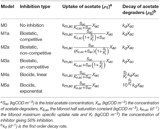
Table 1. Description of kinetic process used in the evaluated models.

We included first order kinetics to describe the biomass decay rate (ρ₅, kgCOD m⁻³ d⁻¹) in all models. Additionally, in models M4a and M5a we described the biocidal inhibition by relating the concentration of inhibitor with the first order decay rate. Therefore, as shown in Table 1, we proposed a simple linear model between the first order decay rate and the concentration of inhibitor in the bulk liquid S_I in M4a, and an exponential term in M5a. The latter was analogous to the microbial inactivation kinetics by chemical compounds (Casolari, 1988).

Liquid-Gas Mass Transfer

We estimated the specific liquid-gas mass transfer rates for methane (ρ₂, kgCOD m⁻³ d⁻¹), carbon dioxide (ρ₃, kmol m⁻³ d⁻¹), and nitrogen (ρ₄, kmol m⁻³ d⁻¹) as follows (Batstone et al., 2002):

$\begin{array}{ll}{\rho }_2=k_{L}a(S_{ch4}-K_{H,ch4}{p}_{gas,ch4})& (3)\end{array}$

$\begin{array}{ll}{\rho }_3=k_{L}a(S_{co2}-K_{H,co2}{p}_{gas,co2})& (4)\end{array}$

$\begin{array}{ll}{\rho }_4=k_{L}a(S_{n2}-K_{H,n2}{p}_{gas,n2})& (5)\end{array}$

where k_La is the dynamic gas–liquid transfer coefficient, K_H,n2 (kmol m⁻³ bar⁻¹), K_H,co2 (kmol m⁻³ bar⁻¹), and K_ch4 (kgCOD m⁻³ bar⁻¹) are the Henry's law coefficients, p_gas,ch4, p_gas,co2 and p_gas,n2 (bar) the partial pressures of gases, and S_ch4 (kgCOD m⁻³), S_co2 (kmol m⁻³), and S_n2 (kmol m⁻³) the concentrations of methane, carbon dioxide and nitrogen in the liquid phase, respectively. We assumed the same value for k_La for all gaseous components.

We estimated the composition of the gas phase assuming that gas-liquid equilibrium was reached for all gaseous components in accordance to Henry's law, and that the total gas pressure p_gas (bar) was the sum of the partial pressures of all the gaseous components inside the reactor. Consequently, we estimated the partial pressure p_gas,i as follows:

$\begin{array}{ll}{p}_{gas,i}=p_{gas}\frac{\frac{S_i}{K_{H,i}}}{\frac{S_{n2}}{K_{H,n2}}+\frac{S_{ch4}}{K_{H,ch4}}+\frac{S_{co2}}{K_{H,co2}}}& (6)\end{array}$

We used the acid-base equilibrium equation for inorganic carbon (CO_2,ac/HCO${}_3^{-}$) to estimate the S_co2 from the concentration of inorganic carbon in the liquid phase (S_IC, kmol m⁻³), as follows:

$\begin{array}{ll}{S}_{c{o}_2}=S_{IC}\left(1-\frac{K_{a,c{o}_2}}{K_{a,c{o}_2}+10^{-pH}}\right)& (7)\end{array}$

where K_{a, CO2} (-) is the acid-base equilibrium coefficient and pH (-) is the pH of the solution. In this research, we considered a constant pH, because we added a pH-buffer into the bottles in the batch-tests experiments.

Mass Balances

We estimated the AMP (P_ch4, kgCOD kgVSS⁻¹) from the specific liquid-gas mass transfer rates (ρ₂), as follows:

$\begin{array}{ll}\frac{\partial P_{ch4}}{\partial t}=\frac{{\rho }_2}{t_{c}X(0)}& (8)\end{array}$

where X(0) (kgVSS m⁻³) is the initial concentration of VSS in the reactor, experimentally determined, and t_c (86,400 s d⁻¹) is a time conversion factor.

We used the following mass balance equation for component i in the bulk liquid:

$\begin{array}{ll}\frac{\partial C_{B,i}}{\partial t}=\frac{1}{t_c}{\displaystyle \sum _{j=\left[1-6\right]}}{\nu }_{ij}{\rho }_j& (9)\end{array}$

where C_B,i is the concentration of the soluble (S_i) or particulate (X_i) component i in the bulk liquid, t (s) the time, ν_ij the stoichiometric coefficients of component i on process j and ρ_j (kgCOD m⁻³ d⁻¹ or kmol m⁻³ d⁻¹) the rate of process j. The ν_ij are presented in Table 2.

TABLE 2

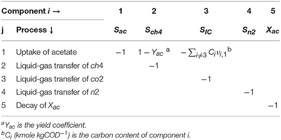
Table 2. Stoichiometric coefficients (υ_{i, j}).

Model Implementation

Computational Implementation

We performed all computations in Matlab^® R2018a and used the built in ordinary differential equations (ODE) solver ode15s to integrate the ordinary differential equations system. The initial conditions and parameters of the experiments needed for model resolution were: p_gas, pH, V, M_R, C₀, S_i(0) and X_ac(0). We calculated the SMA simulations (kgCOD kgVSS⁻¹ d⁻¹) as the maximum methane production rate, as follows:

$\begin{array}{ll}\text{SMA prediction}=\text{max}(\frac{\Delta P_{ch4}}{\Delta t}{t}_c)& (10)\end{array}$

We estimated the goodness of fit based on the sum of squared errors (SSE), as follows:

$\begin{array}{ll}\text{SSE}={\sum }_i{(y_{e,i}-y_{m,i})}^2& (11)\end{array}$

where y_e,i is the experimental observation i and y_m,i the corresponding model prediction. We estimated the SSE both using SMA as the output variable (SSE-SMA, kgCOD² kgVSS⁻² d⁻²) and using the AMP as output variable (SSE-AMP, kgCOD² kgVSS⁻²). We used different polymer concentrations C₀ in each SMA tests (see section Batch Reactor Tests); thus, we solved the models (M1a to M5a) individually for each C₀ tested to estimate the SSE.

As described in section Batch Reactor Tests, the AMPTS generates a digital pulse after a fixed volume of gas has flowed through the gas cells; consequently, the time at which each data point was measured was different for each bottle, even for the triplicates of the same SMA test. Therefore, to estimate the SSE-AMP, the models needed to predict the methane production at the exact experimental time instant. To achieve this, the models were solved with a sufficiently small time step (that is t = 1000 s), and the AMP prediction values were linearly interpolated at the exact experimental time instants for each SMA bottle.

Nominal Values of Parameters

The values of most parameters were obtained from literature, and are summarized in Table 3. The values of parameters related to the polymer characteristics, namely Q_m, K_L, and K_I, were selected based on specific assumptions, and the most influential ones estimated to fit the experimental data. There are several commercial cationic polymers with similar compositions but each of them with different charges and molecular weights. To our best knowledge, there are no specific values for the parameters related to the polymer characteristics reported in literature. The parameters for the Langmuir adsorption model, Q_m and K_L, are conditioned to the type of adsorbent and adsorbate. We used experimental data for the adsorption of polyDADMAC onto different adsorbents from previous reports and estimated the values of Q_m and K_L. The estimated values of Q_m were 0.032, 0.450, and 0.035 kg kg⁻¹ for adsorption onto silica gel of 6 nm pore size (Hubbe et al., 2011), activated sludge (Zhao et al., 2016), and cellulosic fibers (Horvath et al., 2006), respectively, and those for K_L were 2.0, 7.6 and 1,960 m³ kg⁻¹, respectively. Q_m and K_L results were highly dispersed, therefore we used the values proposed for adsorption onto activated sludge as an initial guess. We assumed the K_I equal to the C_e calculated using Equation (1) and Equation (2) by substituting for the values for Q_m and K_L from activated sludge and for the value for C₀ equal to the experimental concentration of polymer at which the SMA value was 50% smaller than the SMA without polymer. Therefore, the K_I was set equal to 0.014 kgCOD m⁻³.

TABLE 3

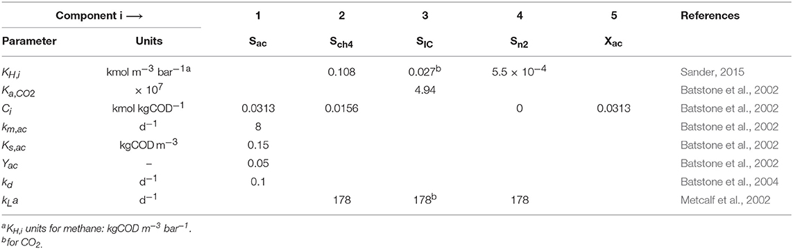
Table 3. Nominal parameter values at 35°C.

Initial Conditions and Experimental Parameters

We estimated the total solids content inside the reactor (M_R, kgTSS) as the initial concentration of TSS in the reactor, which was experimentally determined, times the liquid volume of the reactor (V). The initial concentration C₀ in Equation (2) represents the concentration of polymer added to the SMA bottles. We assumed a constant total gas pressure p_gas equal to the mean experimentally measured pressure, which was 1.01 bar. We introduced the ratio between partial pressure and total gas pressure at time zero as an initial condition in each model and estimated the soluble components concentrations [S_ch4(0), S_IC(0) and S_co2(0)] using Equations (6) and (7), assuming that the system starts at gas-liquid equilibrium. Since the bottles were initially flushed with nitrogen gas, we assumed that the initial $\frac{p_{gas,i}}{p_{gas}}$ were 0, 0 and 1 for methane, carbon dioxide and nitrogen, respectively.

We calculated the initial concentration of acetate degraders as X_ac(0) = f_Xac,0 VSS(0), where f_Xac,0 (kgCOD kgVSS⁻¹) is the initial fraction of acetate degraders of the VSS. We estimated the f_Xac,0 value to fit the model M0 (Table 1) to the experimental AMP when no polymer was added to the SMA bottles. We did not include the adsorption model since no polymer was present in the reactor. We estimated the initial guess assuming that all the methane produced from acetate left the bottles and considering S_ac≫K_s,ac. Consequently, the initial guess for f_Xac,0 was estimated as follows:

$\begin{array}{ll}{f}_{Xac,0}=\frac{\text{SMA}}{k_{m,ac}(1-Y_{ac})}& (12)\end{array}$

where the SMA (kgCOD kgVSS⁻¹ d⁻¹) was experimentally measured.

Models Calibration

As described in sections Nominal Values of Parameters and Initial Conditions and Experimental Parameters, we estimated the parameters f_Xac,0, Q_m, K_L and K_I to fit the experimental data. We used the AMP without polymer addition as the model output (y) to estimate f_Xac,0, and for the remaining parameters we used SMA for different initial polymer concentrations C₀ as the model output.

We carried out the model calibration in five steps, namely: (1) identification of a parameter subset (θ) containing only the influential parameters based on the standardized regression coefficients (β_i) from the linear regression model built using the MC simulations; (2) definition of the boundaries for the parameters based on the behavior of the SSE with respect to uncertain model parameters; (3) parameter estimation (PE) with θ and evaluation of the quality of the estimators; (4) (when needed) identification of the θ that can be reliably estimated from the given experimental data, by modification of the model structure and/or identifiability analysis; and (5) PE with new θ and/or model. Additionally, we performed a model prediction uncertainty analysis using the MC method with the parameter uncertainty obtained from PE.

Monte Carlo and Linear Regression

We performed a global sensitivity analysis to identify the effect of the parameters on the model output. We executed the analysis based on linear regression models built from MC simulations. We defined the input uncertainty as a uniform distribution with 99.9 % variability, we used 99.9 % instead of 100 % to avoid null values; zero values for some parameters would cause numerical problems, for example, if K_H,i is zero (for any i) then there is a division by zero in Equation (6). Consequently, the minimum and maximum value of the distributions were 0.001θ° and 1.999θ°, respectively, where θ° is the initial/nominal parameter vector. The notation θ ~ U(0.001θ°, 1.999θ°) is further used in this document. The θ included all parameters in each model. We used Latin hypercube sampling (Iman and Conover, 1982) with 500 samples (Sin et al., 2009); computed the β_i using the mean-centered sigma-scaling (Helton and Davis, 2003), and estimated the β_i using the constrained linear least square minimization function lsqlin with −1 and 1 as lower and upper bound, respectively. The estimation of the β_i requires a scalar input; therefore we computed the β_i individually for each C₀ in M1a to M5a and for each time (t) in M0. We used the coefficient of determination (R²) to evaluate the quality of the regression model, that is: the model was considered sufficiently linear when R² ≥ 0.7 (Sin et al., 2011). We calculated the mean, minimum and maximum R² with the β_i obtained for each parameter in the range of C₀ or t were R² ≥ 0.7. The parameters with a mean abs(β_i) ≥ 0.10 were considered influential (Sin et al., 2011).

Parameter Estimation

We studied the behavior of the SSE with the parameter values in the subset θ varying in a wide range to research the existence of local minimums and determine the boundaries and initial guess for the PE. We performed MC simulations with Latin hypercube sampling with 500 samples, using a uniform distribution with 99.9% variability for the parameter subset defined in section Monte Carlo and Linear Regression and calculated the SSE for each simulation. We defined the range of the parameters based on the behavior of the SSE with respect to uncertain model parameters.

Subsequently, we estimated the parameters using the non-linear least squares solver lsqnonlin in Matlab^® R2018a, using the trust region reflective algorithm and with the lower and upper bounds previously identified. The input function for the lsqnonlin solver was an array with the residuals, where Residuals = y_e−y_m. Afterwards, the solver found the optimal value ($\widehat{\theta }$) that minimizes the sum of squares of the input function, consequently, it minimizes the SSE in Equation (11). We calculated the standard deviation (σ_θ) and 95 % confidence interval (CI) of the estimators in accordance to Sin and Gernaey (2016).

The normality of the residuals needs to be evaluated since it is an underlying hypothesis for the implementation of least square method for parameter estimation. We assessed the distribution of the residuals graphically and used Shapiro-Wilk test to test the hypothesis of normality using the function swtest ^© (BenSaïda, 2009). When the null hypothesis of normality was rejected at a significance level 0.05, we estimated the parameters using bootstrap method, implemented as described in Sin and Gernaey (2016).

We assessed the quality of the estimators based on the uncertainty of the estimators and the pairwise linear correlation between the parameters and considered a good estimation when the relative error, namely $\frac{{\sigma }_{\theta }}{\widehat{\theta }}$, was below 10 % and a poor estimation when it was above 50 % (Sin and Gernaey, 2016). Additionally, if the correlation coefficient between any pair of parameters was above 0.5, we assumed that the PE problem was ill conditioned. Then, we performed an identifiability analysis to select the parameter subset that can be identified uniquely from the experimental data. Therefore, we computed the collinearity index of the parameter subset k (γ^k) (Sin and Gernaey, 2016). The threshold to select a uniquely parameter subset is reported between 5 and 15 (Sin and Gernaey, 2016). We selected the parameter subset with γ^k below 10 for the PE.

Modeling Scenarios

Two different scenarios were studied. The first scenario (models a: M1a, M2a, M3a, M4a, and M5a), considered that the inhibition is caused by the polymer (inhibitor) present in the bulk liquid. As described in section Polymer Adsorption, when a polymer is added to a sludge sample a fraction of the polymer is adsorbed onto the sludge and a fraction remains in the bulk liquid. The concentration of polymer in the bulk liquid after the adsorption reaching equilibrium is C_e, and C_e was considered as the concentration of polymer responsible for the inhibition in the first scenario, namely S_I = C_e.

In the second scenario (models b: M1b, M2b, M3b, M4b, and M5b), the inhibition was assumed to be caused by the total amount of polymer added to the SMA bottles. The inhibition is caused by both the fraction of polymer adsorbed onto the sludge and the fraction remaining in the bulk liquid. Consequently, the adsorption model was not needed to describe the inhibition and it was removed from the model structure in models b and the S_I was set equal to the total concentration of polymer added to the SMA bottles (C₀), namely S_I = C₀.

Model Prediction Uncertainty

We selected the most suitable models based on the model capacity to predict the experimental data (goodness of fit), which was assessed graphically and with the SSE-SMA and SSE-AMP. For the selected models, we studied the model prediction uncertainty caused by the uncertainty in the estimators, using the MC method with Latin hypercube sampling. We defined the uncertainty in the parameters using the results from the PE, as a normal distribution with mean $\widehat{\theta }$ and standard deviation σ_θ, namely $\theta ~N(\widehat{\theta },{{\sigma }_{\theta }}^2)$, and represented the uncertainty propagation graphically.

Results

Experimental Results

The polymer presented an inhibitory effect on the SMA. The SMA of the sludge without polymer was 0.219 gCOD gVSS⁻¹ d⁻¹. A 50 % SMA inhibition was obtained at 0.27 gCOD L⁻¹ of polymer, the value was obtained by linear interpolation (see Supplementary Material). No significant effect was observed in the AMP achieved at the end of the tests, for further information see the Supplementary Material.

Modeling AMP Without Polymer Addition (M0)

The linear regression models built using the MC simulations of M0 resulted in R² above 0.7 between 2 and 79 h. The mean, minimum and maximum β_i values for the range with R² > 0.70 are presented in Table 4. The SSE-AMP was calculated for each MC simulation and the results are presented in Figure 1. The behavior of the SSE-AMP with f_Xac,0, for uncertainty only in f_Xac,0, is shown in Figure 1C.

TABLE 4

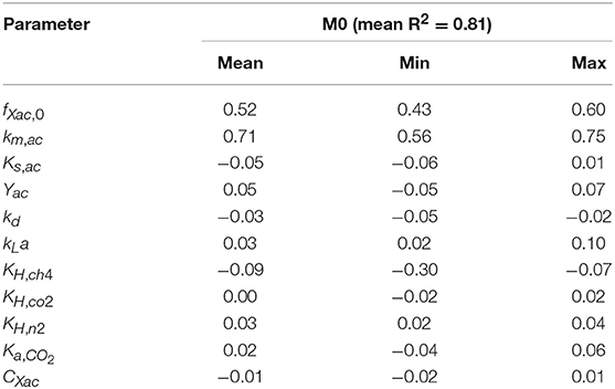
Table 4. Sensitivity analysis results for M0: mean, minimum (min) and maximum (max) of the standardized regression coefficients (β_i) of linear models with R² > 0.7 of AMP as a function of time.

FIGURE 1

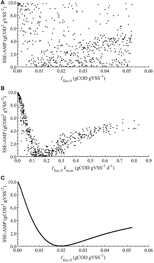
Figure 1. Correlations between the SSE-AMP and uncertain parameters with θ ~ U(0.001θ°, 1.999θ°) for M0: correlation of SSE-AMP with f_Xac,0 (A) and SSE-AMP with f_Xac,0k_m,ac (B) using MC simulations performed with uncertainty in all parameters; correlation of SSE-AMP with f_Xac,0 using MC simulations performed with uncertainty only in the f_Xac,0 (C).

The initial guess for f_Xac,0 estimation was 0.02, and the lower and upper bounds were 0.01 and 0.03, respectively. The PE results were as follows: 0.0198 kgCOD kgVSS⁻¹ optimal value ($\widehat{\theta }$), 1.9 × 10⁻⁴ standard deviation (σ_θ), 3.8 × 10⁻⁴ 95 % confidence interval (CI) and relative error $\frac{{\sigma }_{\theta }}{\widehat{\theta }}$ of 1 %. We performed PE varying the initial guess and the same results were obtained. The null hypothesis of normality was rejected at a significance level 0.05 using the Shapiro-Wilky test with a p-value of 2 × 10⁻⁷. The optimal value obtained using Bootstrap was equal to the one obtained with least squares method, namely 0.0198 kgCOD kgVSS⁻¹. Figure 2 displays the experimental AMP and the model predictions at the optimal values obtained with PE. Although the experimental data was collected over a 10-day period, not enough biogas to generate a new pulse in the AMPTS was produced in the bottles after 80 h, further explanation was presented in Supplementary Material.

FIGURE 2

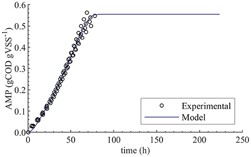
Figure 2. Experimental and simulated AMP in the absence of polymer (M0). Simulations performed with the optimum value obtained from parameter estimation, namely f_Xac,0 = 0.0198 kgCOD kgVSS⁻¹.

Modeling the Methanogenesis Inhibition by the Polymer

The results from the linear models performed with the MC simulations with parameter uncertainty θ ~ U(0.001θ°, 1.999θ°) are summarized in Table 5. From the parameters present in the initial subsets θ, the ones with mean β_i ≥ 0.10 were: {K_I, K_L, Q_m} in M1a to M4a and {K_I, K_L} in M5a.

TABLE 5

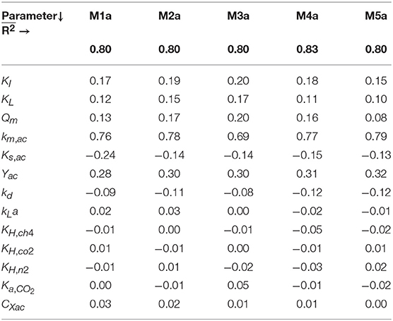
Table 5. Sensitivity analysis results for M1a to M5a: mean of the standardized regression coefficients (β_i) and mean R² ($\overline{R^2}$) of linear models with R² > 0.7 of the SMA with different concentrations of polymer.

The results from the PE in M1a to M5a are shown in Table 6. Figure 3 shows the comparison between the best-fit results of the five models and the experimental data. The correlation coefficients and collinearity index for all the possible combinations of parameters are summarized in Table 7. Based on the results, a new parameter subset was defined containing only K_I, and the values of K_L and Q_m were set at their nominal values (defined in section Nominal values of parameters)

TABLE 6

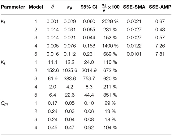
Table 6. Parameter estimation results for the SMA inhibition for M1a to M4a with parameter subset θ = {K_I, K_L, Q_m} and M5a with θ = {K_I, K_L}: optimal values ($\widehat{\theta }$), standard deviation (σ_θ) and 95% confidence intervals (CI); and sum of square errors for SMA (SSE-SMA) and AMP (SSE-AMP) of the models.

FIGURE 3

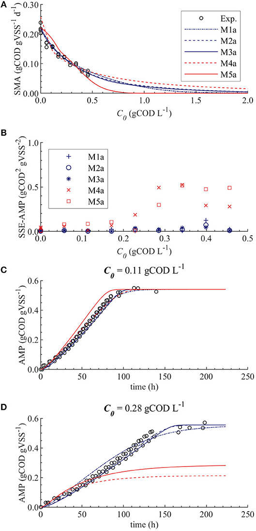
Figure 3. Simulations with parameter estimation results for the SMA inhibition for M1a to M4a with parameter subset θ = {K_I, K_L, Q_m} and M5a with parameter subset θ = {K_I, K_L}: experimental and simulated SMA (A), SSE-AMP (B), experimental and simulated AMP at 0.11 gCOD L⁻¹ of polymer (C) and experimental and simulated AMP at 0.28 gCOD L⁻¹ (D).

TABLE 7

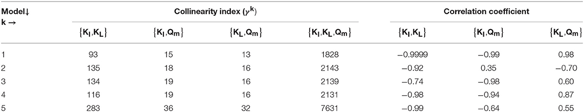
Table 7. Correlation and collinearity index for M1a to M5a for different parameter combinations k.

Figures 4A,B display the behavior of the SSE for SMA with $K_I~U(0.001\theta °,1.999\theta °)$ for models a (M1a, M2a, M3a, M4a, and M5a) and b (M1b, M2b, M3b, M4b, and M5b), respectively. The results from the PE estimation are summarized in Table 8. Figure 5 compare between the best-fit results of the models with the experimental data.

FIGURE 4

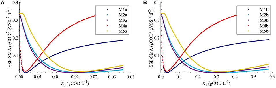
Figure 4. Correlations between the SSE-SMA and uncertain parameters using MC simulations with uncertainty θ ~ U(0.001θ°, 1.999θ°) only in K_I. Results using M1a to M5a (A) and M1b to M5b (B).

TABLE 8

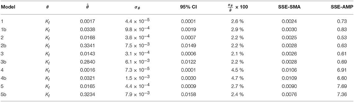
Table 8. Parameter estimation results for the SMA inhibition process with parameter subset θ for M1a to M5a (with S_I = C_e) and M1b to M5b (with S_I = C₀).

FIGURE 5

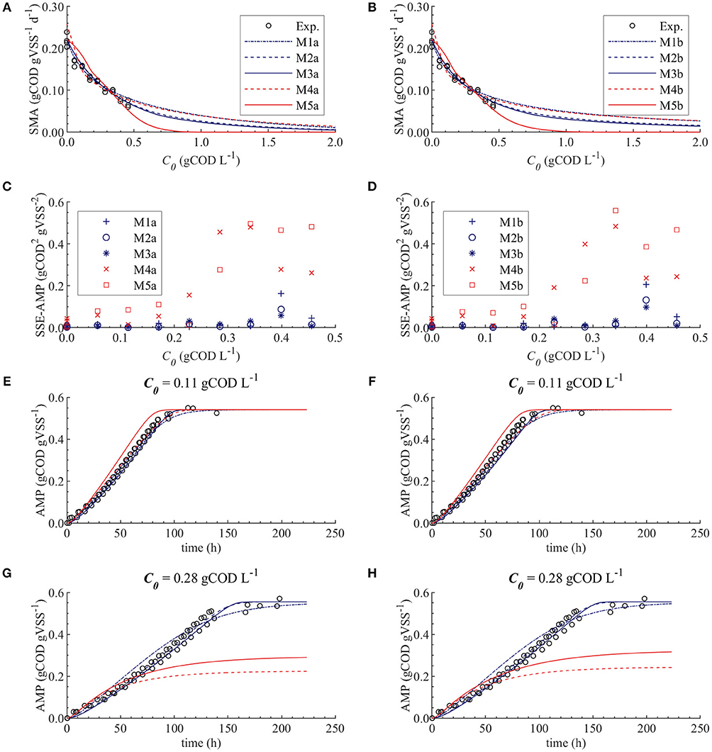
Figure 5. Simulations with parameter estimation results for the SMA inhibition, with parameter subset θ = {K_I}: experimental and simulated SMA for M1a to M5a (A) and M1b to M5b (B), SSE-AMP for M1a to M5a (C) and M1b to M5b (D), experimental and simulated AMP at 0.11 gCOD L⁻¹ of polymer for M1a to M5a (E) and M1b to M5b (F) and experimental and simulated AMP at 0.28 gCOD L⁻¹ for M1a to M5a (G) and M1b to M5b (H).

Model Prediction Uncertainty

The uncertainty in the M2a and M2b predictions caused by the uncertainty in K_I, with $\theta ~N(\widehat{\theta },{{\sigma }_{\theta }}^2)$, are compared with the experimental data in Figure 6.

FIGURE 6

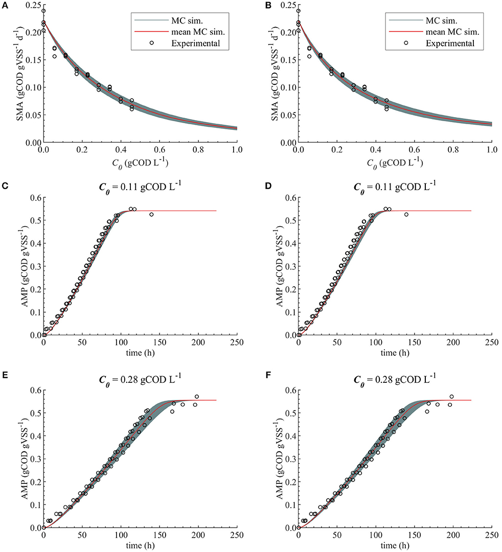
Figure 6. Monte Carlo simulations with uncertainty $\theta ~N(\widehat{\theta },{{\sigma }_{\theta }}^2)$ and subset θ = {K_I} for M2a and M2b. Experimental data, MC simulations (MC sim.) and mean MC simulations for: SMA for M2a (A) and M2b (B), AMP at 0.11 gCOD L⁻¹ of polymer for M2a (C) and M2b (D) and AMP at 0.28 gCOD L⁻¹ for M2a (E) and M2b (F).

Discussion

In this research, we assessed the inhibition of SMA and AMP caused by cationic polymer addition to anaerobic sludge. The results showed that the polymer inhibited the SMA but did not have an effect on the final AMP achieved. The experimental results are further presented in the Supplementary Material.

To the authors best knowledge, two reports are available that use Adipap polymers for fouling control in membrane bioreactors. Significant fouling decrease was achieved by adding 0.05 gCOD L⁻¹ of KD451 to a pilot AnMBR (Odriozola et al., 2019) and 70 mg L⁻¹ (0.077 gCOD L⁻¹) of KD452 to a pilot MBR (Iversen et al., 2009). These concentrations are considerably below the 50 % SMA inhibition concentration, namely 0.27 gCOD L⁻¹. However, we obtained 24 and 27 % SMA inhibitions at 0.06 and 0.11 gCOD L⁻¹ of polymer concentration, respectively. Consequently, in a continuous AnMBR reactor, adding polymer might decrease the methane production rate, increase the acetate concentration and decrease the organic matter removal when organic loading rates remain at the same level. The effect would start immediately after addition and it can be compensated by a decrease in the organic volumetric loading rate. Additionally, if the inhibition is reversible (biostatic) the overall conversion capacity of the bioreactor could be recovered by an increase in the biomass content. If the methanogenic microorganisms are in excess when adding the polymer to the AnMBR then the methane production, acetate concentration and organic matter removal might not be affected by small dosages of polymer.

Validity of Nominal Values of Parameters

The results from the global sensitivity analysis showed that a 99.9% variability on the gas-liquid transfer (k_La, K_H,i) and carbon content (C_Xac) parameters had a negligible effect (β_i < 0.10) on the SMA inhibition (Table 5) and on the AMP without polymer (Table 4). Consequently, for those parameters, the selection of the exact (true) parameter values was not crucial and we considered it acceptable to use the nominal parameter values from literature presented in section Nominal Values of Parameters.

Contrarily, the kinetic and stoichiometric parameters related to acetate degradation and biomass decay presented a significant effect on the model output. Particularly, the Monod maximum specific uptake rate k_m,ac was the most influential parameter in all considered models. The f_Xac,0 was highly correlated with k_m,ac, meaning that the optimal value for f_Xac,0 is determined by the value of k_m,ac used (Figure 1B). Although, good model fits could be obtained with different combinations of f_Xac,0 and k_m,ac, this was outside the scope of this research. In this manuscript, we focused on modeling the SMA inhibition and comparing different inhibition models and not on the acetoclastic methanogenesis kinetics itself. Therefore, we used widely applied values for k_m,ac, Y_ac, K_s,ac and k_d, presented in section Nominal Values of Parameters.

Modeling AMP Without Polymer Addition (M0)

The initial fraction of acetate degraders of the VSS (f_Xac,) showed a significant effect on the AMP model output (Table 4): 28 % (${{\beta }_i}^2\times 100$) of the output variability could be explained by the variability on f_Xac,0. Therefore, we could estimate the f_Xac,0 to predict the methane production obtained experimentally. Results did not show a clear pattern of the behavior of SSE-AMP with f_Xac,0 with uncertainty in all parameters (Figure 1A). However, the SSE-AMP with f_Xac,0 with uncertainty only in f_Xac,0 (Figure 1C) showed a unique (global) minimum value at f_Xac,0 around 0.02 gCOD gVSS⁻¹. Parameter estimation results showed that the quality of the estimator is good since the relative error was small and the model predictions fit the experimental data, as shown in Figure 2.

Calibration of SMA Inhibition Models

Ill Conditioned Models

We identified the influential unknown parameters, for PE, using the results from the sensitivity analysis (Table 5). The subsets identified, with a threshold value of the mean β_i ≥ 0.10, are as follows: θ = {Q_m, K_L, K_I} in M1a to M4a and θ = {K_L, K_I} in M5a.

The SMA simulations, at the optimal values obtained with PE, showed a good fit to the experimental data for the biostatic models (M1a, M2a and M3a) and the biocide-lineal model (M4a), as observed in Figure 3A. Accordingly, Figure 3C shows a good fit to the experimental AMP with M1a to M4a for a polymer concentration of 0.11 gCOD L⁻¹. However, for higher concentrations (Figure 3D) the M1a simulations slightly deviated from the experimental data, and the M4a simulations were considerably below the experimental data after 50 h. The previous deviations are reflected by the SSE-AMP in Figure 3B. The accelerated biomass decay predicted in M4a caused a noticeably low concentration of microorganisms resulting in an extremely low methane production rate after 50 h. Similarly, in M5a the AMP was underpredicted for high concentrations of polymer. Additionally, the biocide-exponential model (M5a) overpredicted and underpredicted the SMA at polymer concentrations C₀ below and above 0.3 gCOD L⁻¹, respectively.

Models a (M1a to M5a) considered the inhibition caused by the concentration of inhibitor in the bulk liquid S_I, where S_I was determined by the Langmuir isotherm adsorption model (section Polymer Adsorption). Consequently, as expected, high pairwise correlation coefficients were obtained for all parameter combinations (Table 7). As a result, the relative errors obtained with PE were considerably high (Table 6). Therefore, although some of the models were able to predict the experimental data, the quality of the estimators was considered poor, namely the relative error was above 50 % (Sin and Gernaey, 2016).

From the collinearity indexes presented in Table 7, no combination of parameters could be used to achieve unique estimators from the experimental data, namely γ^k > 10 for all k. Therefore, we performed a new PE with a subset containing only one parameter. We selected the inhibition coefficient K_I for the PE because it presented a slightly higher effect on the simulated SMA (higher mean β_i, Table 5) compared to Q_m and K_L, and we used the nominal Q_m and K_L values. The simulation results with the optimal values obtained with PE (Figure 5, on the left) were very similar to the ones obtained at the optimal values from PE using θ = {Q_m, K_L, K_I} (or θ = {K_L, K_I} in M5a), Figure 3.

Additionally, we considered a different inhibition approach, where the inhibition was assumed to be caused by the total amount of polymer added to the SMA bottles, namely S_I = C₀. Therefore, we defined the models b (M1b to M5b) and compared them with the original models a (M1a to M5a), where S_I = C_e. In Figure 5 the simulation results for models a and b are displayed on the left and right graphs, respectively; the results are further discussed in section Bulk Liquid vs. Total Polymer Concentration Inhibition.

Biostatic and Biocidal Inhibition Models

As we discussed in section Ill Conditioned Models, biocide models (M4a and M5a) underpredicted the experimental methane production at high polymer concentrations due to the accelerated biomass decay. Therefore, the biocide models M4a and M5a were not appropriate models to describe the inhibition of methanogenesis by the polymer. Contrarily, predictions with biostatic models (M1a, M2a, and M3a) showed satisfactory fit to the experimental SMA and AMP (Figure 5). Therefore, it is likely that the polymer inhibition on the SMA is a reversible process (biostatic inhibition), instead of a reactive irreversible toxicity (biocidal inhibition). Consequently, in a continuous reactor, the inhibitory effect will be eliminated when the polymer concentration decreases. Additionally, based on the dosage of the polymer and the microbial growth rate, the overall microbial activity could be recovered by an increase in the biomass content.

Figure 5A shows that the simulations using the un-competitive (M3) and non-competitive (M2) inhibition models successfully fitted all the experimental SMA, while the competitive inhibition model (M1a) simulations slightly deviate from the SMA at the higher concentrations of polymer tested, namely 0.40 and 0.46 gCOD L⁻¹. Additionally, Figure 5G shows that the M5a overpredicted the AMP between 40 and 100 h at 0.28 gCOD L⁻¹, while the M2a and M3a model simulations fitted the AMP remarkably well.

Therefore, although the M1a fitted the experimental data significantly well, the process was better described by M2a and M3a. Additionally, as the competitive inhibition model (M1) considers that the inhibitor binds to the same place as the substrate (Garcia Orozco, 2008), and because the polymer (inhibitor) and the acetate (substrate) are different molecules, the latter result was not unexpected.

The difference between the un-competitive and non-competitive models could only be observed in the AMP predictions at high concentration of polymer (Figure 5G). Based on the SSE presented in Table 8 the M2a seems to predict slightly better the experimental data. However, the difference was not considered sufficient to select one model over the other and both models were considered appropriate to describe the methanogenesis inhibition process.

Bulk Liquid vs. Total Polymer Concentration Inhibition

The behavior of the SSE-SMA with K_I revealed a unique (global) minimum for all models. Figure 4 displays the SSE-SMA as a function of K_I for models with inhibition by the concentrations of polymer in the bulk liquid (Figure 4A) and by the total amount of polymer added to the system (Figure 4B). Results presented a similar behavior for both inhibition models, however, the K_I values that minimize the SSE-SMA are 20 times larger for the models with S_I = C₀, which corresponds to the ratio between the C₀ and C_e obtained by applying the adsorption model (section Polymer Adsorption) with the nominal parameter values and experimental conditions.

Parameter estimation results showed that the models a (with S_I = C_e) presented a slightly smaller SSE-SMA and SSE-AMP for each biostatic inhibition model considered with respect to the models b (with S_I = C₀), as shown in Table 8. However, the difference in the simulations with the models a (left plots) and models b (right plots) was negligible for each kinetic inhibition model used, as observed in Figure 5. The similarity between models a and b was due to the approximately linear relationship between C₀ and C_e obtained using the polymer adsorption model (results not shown). This approximately linear behavior was obtained using the experimental conditions tested (C₀, M_R, and V) and with the Langmuir parameter values obtained by parameter estimation (K_L and Q_m).

Therefore, both modeling approaches (bulk liquid or total polymer concentration inhibition) were considered appropriate to describe the methanogenesis inhibition caused by the polymer in the range of concentrations studied. Additionally, the uncertainty in the estimated parameters did not cause a considerable uncertainty on the model prediction for M2a and M2b, Figure 6.

Conclusion

The cationic polymer showed a negative effect on the biological activity of the anaerobic sludge. A 50 % SMA inhibition was obtained at 0.27 gCOD L⁻¹ of polymer whereas no significant effect on the final AMP was observed.

Different models were presented and calibrated to fit the experimental data. The Monte Carlo method was successfully applied to study the sensitivity of the model outputs to the parameters and identify the parameter subsets for parameter estimation. The collinearity indexes and pairwise correlation coefficients showed that the parameters Q_m, K_L and K_I are all highly correlated. Based on the Monte Carlo results and collinearity indexes the parameter subsets selected for parameter estimation was θ = {K_I} for all the models considered.

We studied an alternative modeling approach, models M1b to M5b, considering that the inhibition was caused by the total amount of polymer added to the reactor (S_I = C₀), and not by the concentration that remains in the bulk liquid after adsorption (S_I = C_e, M1a to M5a). The difference in the models simulations with both approaches, namely S_I = C_e and S_I = C₀, was negligible for each kinetic inhibition model used.

The simulated AMP values obtained with the biocide models, namely M4a and M5a, were below the experimental AMP at high concentrations of polymer, which was caused by a rapid decay of the acetate degraders simulated. The only models that adequately fitted the experimental SMA and AMP were the non-competitive (M2a and M2b) and un-competitive (M3a and M3b) inhibition models. Therefore, it is likely that the polymer inhibition on the SMA is reversible, instead of toxic and irreversible.

The concentrations of polymer (inhibitor) in the bulk liquid giving 50 % inhibition were 0.014 and 0.017 gCOD L⁻¹ for M2a and M3a, respectively; and the total concentrations of inhibitor in the reactor giving 50 % inhibition were 0.334 and 0.284 gCOD L⁻¹ for M2b and M3b, respectively.

The simulated SMA obtained with M1a and M4a adequately fitted the experimental SMA. However, the simulated AMP was below the experimental AMP for those models. Therefore, it is crucial to analyze both outputs, SMA and AMP, during model calibration.

Author Contributions

MO designed and performed the experiments. MO, EA, and HS derived the model and MO performed the computational implementation. MO, EA, HS, ML-F and JvL provided critical feedback and helped shape the research, analysis and manuscript.

Funding

This research is financially supported by the European Union through the ERANET Cofund activity entitled Bioenergy Sustaining the Future (BESTF14002) in the framework of the project BIO-METHANE PRODUCTION FROM URBAN ORGANIC MATTER. The authors gratefully acknowledge the personal scholarship from the Agencia Nacional de Investigación e Innovación (ANII), Uruguay, to MO (POS_EXT_2015_1_123999).

Conflict of Interest Statement

The authors declare that the research was conducted in the absence of any commercial or financial relationships that could be construed as a potential conflict of interest.

Supplementary Material

The Supplementary Material for this article can be found online at: https://www.frontiersin.org/articles/10.3389/fbioe.2019.00093/full#supplementary-material

References

American Public Health Association, American Water Works Association. Water Environment Federation. (1999). Standard Methods for the Examination of Water and Wastewater. 20th ed, ed. A. D. Cleseceri, S, Leonore, Greenberg, Arnold, E. (Eaton Washington DC: APHA/AWWA/WEF).

Google Scholar

Astals, S., Batstone, D. J., Tait, S., and Jensen, P. D. (2015). Development and validation of a rapid test for anaerobic inhibition and toxicity. Water Res. 81, 208–215. doi: 10.1016/j.watres.2015.05.063

PubMed Abstract | CrossRef Full Text | Google Scholar

Batstone, D., Keller, J., and Blackall, L. (2004). The influence of substrate kinetics on the microbial community structure in granular anaerobic biomass. Water Res. 38, 1390–1404. doi: 10.1016/j.watres.2003.12.003

PubMed Abstract | CrossRef Full Text | Google Scholar

Batstone, D. J., Keller, J., Angelidaki, I., Kalyuzhnyi, S. V., Pavlostathis, S. G., Rozzi, A., et al. (2002). Anaerobic Digestion Model No.1 Adm1: IWA Task Group for Mathematical Modelling of Anaerobic Digestion Processes. London: IWA Publishing.

Google Scholar

BenSaïda, A. (2009). Shapiro-Wilk and Shapiro-Francia normality tests. MATLAB Cent. File Exch. Available online at: https://nl.mathworks.com/matlabcentral/fileexchange/13964-shapiro-wilk-and-shapiro-francia-normality-tests (accessed September 1, 2018).

Google Scholar

Casolari, A. (1988). “Microbial death,” in Physiological Models in Microbiology, eds. M. Bazin, and J. I. Prosser, (Boca Raton, FL, USA: CRC Press), 1–44.

Google Scholar

Dereli, R. K., Ersahin, M. E., Ozgun, H., Ozturk, I., Jeison, D., van der Zee, F., et al. (2012). Potentials of anaerobic membrane bioreactors to overcome treatment limitations induced by industrial wastewaters. Bioresour. Technol. 122, 160–170. doi: 10.1016/j.biortech.2012.05.139

PubMed Abstract | CrossRef Full Text | Google Scholar

Díaz, H., Azócar, L., Torres, A., Lopes, S. I. C., and Jeison, D. (2014). Use of flocculants for increasing permeate flux in anaerobic membrane bioreactors. Water Sci. Technol. 69, 2237–2242. doi: 10.2166/wst.2014.153

PubMed Abstract | CrossRef Full Text | Google Scholar

Garcia Orozco, J. H. (2008). “Toxicity,” in Biological Wastewater Treatment: Principles, Modelling and Design, eds. M. Henze, M. C. M. Van Loosdrecht, G. A. Ekama, and D. Brdjanovic, (London, UK: IWA Publishing), 273–290.

Google Scholar

Gregory, J., and Barany, S. (2011). Adsorption and flocculation by polymers and polymer mixtures. Adv. Colloid Interface Sci. 169, 1–12. doi: 10.1016/j.cis.2011.06.004

PubMed Abstract | CrossRef Full Text | Google Scholar

Helton, J. C., and Davis, F. J. (2003). Latin hypercube sampling and the propagation of uncertainty in analyses of complex systems. Reliab. Eng. Syst. Saf. 81, 23–69. doi: 10.1016/S0951-8320(03)00058-9

CrossRef Full Text | Google Scholar

Horvath, A. E., Lindström, T., and Laine, J. (2006). On the indirect polyelectrolyte titration of cellulosic fibers. Conditions for charge stoichiometry and comparison with ESCA. Langmuir 22, 824–830. doi: 10.1021/la052217i

PubMed Abstract | CrossRef Full Text | Google Scholar

Hubbe, M. A., Wu, N., Rojas, O. J., and Park, S. (2011). Permeation of a cationic polyelectrolyte into mesoporous silica. Part 3. Using adsorption isotherms to elucidate streaming potential results. Colloids Surfaces A Physicochem. Eng. 381, 1–6. doi: 10.1016/j.colsurfa.2010.12.052

CrossRef Full Text | Google Scholar

Iman, R., and Conover, W. (1982). A distribution-free approach to inducing rank correlation among input variables. Commun. Stat. Simul. Comput. 11, 311–334.

Google Scholar

Iversen, V., Mehrez, R., Horng, R. Y., Chen, C. H., Meng, F., Drews, A., et al. (2009). Fouling mitigation through flocculants and adsorbents addition in membrane bioreactors: comparing lab and pilot studies. J. Memb. Sci. 345, 21–30. doi: 10.1016/j.memsci.2009.08.014

CrossRef Full Text | Google Scholar

Iversen, V., Mohaupt, J., Drews, A., Lesjean, B., and Kraume, M. (2008). Side effects of flux enhancing chemicals in membrane bioreactors (MBRs): study on their biological toxicity and their residual fouling propensity. Water Sci. Technol. 57, 117-23. doi: 10.2166/wst.2008.660

PubMed Abstract | CrossRef Full Text | Google Scholar

Kooijman, G., Lopes, W., Zhou, Z., Guo, H., de Kreuk, M., Spanjers, H., et al. (2017). Impact of coagulant and flocculant addition to an anaerobic dynamic membrane bioreactor (AnDMBR) treating waste-activated sludge. Membranes. 7:E18. doi: 10.3390/membranes7020018

PubMed Abstract | CrossRef Full Text | Google Scholar

Koseoglu, H., Yigit, N. O., Iversen, V., Drews, A., Kitis, M., Lesjean, B., et al. (2008). Effects of several different flux enhancing chemicals on filterability and fouling reduction of membrane bioreactor (MBR) mixed liquors. J. Memb. Sci. 320, 57–64. doi: 10.1016/j.memsci.2008.03.053

CrossRef Full Text | Google Scholar

Krzeminski, P., Iglesias-Obelleiro, A., Madebo, G., Garrido, J. M., van der Graaf, J. H. J. M., and van Lier, J. B. (2012). Impact of temperature on raw wastewater composition and activated sludge filterability in full-scale MBR systems for municipal sewage treatment. J. Memb. Sci. 423–424, 348–361. doi: 10.1016/j.memsci.2012.08.032

CrossRef Full Text | Google Scholar

Lin, H., Peng, W., Zhang, M., Chen, J., Hong, H., and Zhang, Y. (2013). A review on anaerobic membrane bioreactors: applications, membrane fouling and future perspectives. Desalination 314, 169–188. doi: 10.1016/j.desal.2013.01.019

CrossRef Full Text | Google Scholar

Metcalf, L., Eddy, H. P., Tchobanoglous, G., Burton, F. L., and Stensel, H. D. (2002). Wastewater Engineering: Treatment and Reuse, 4th ed. New York, NY: McGraw Hill.

Google Scholar

Muñoz Sierra, J. D., Oosterkamp, M. J., Wang, W., Spanjers, H., and van Lier, J. B. (2018). Impact of long-term salinity exposure in anaerobic membrane bioreactors treating phenolic wastewater: Performance robustness and endured microbial community. Water Res. 141, 172–184. doi: 10.1016/j.watres.2018.05.006

PubMed Abstract | CrossRef Full Text | Google Scholar

Odriozola, M., Lousada-Ferreira, M., Morales, N., Spanjers, H., and van Lier, J. B. (2019). “Fouling control by flocculant addition based on online measurement of sludge filterability in a pilot AnMBR,” in 16th World Congress on Anaerobic Digestion (Delft).

Google Scholar

Odriozola, M., Lousada-Ferreira, M., Spanjers, H., and van Lier, J. B. (2018). “Towards an Automated Fouling Control by Addition of Flux Enhancers to Anaerobic Sludge,”. in XIII Latin American Workshop and Symposium on Anaerobic Digestion (Medellin).

Google Scholar

Ozgun, H., Dereli, R. K., Ersahin, M. E., Kinaci, C., Spanjers, H., and van Lier, J. B. (2013). A review of anaerobic membrane bioreactors for municipal wastewater treatment : Integration options , limitations and expectations. Sep. Purif. Technol. 118, 89–104. doi: 10.1016/j.seppur.2013.06.036

CrossRef Full Text | Google Scholar

Pavlostathis, S. G., and Giraldo-Gomez, E. (1991). Kinetics of anaerobic treatment: a critical review. Crit. Rev. Environ. Control. 21, 411–490. doi: 10.1080/10643389109388424.

CrossRef Full Text | Google Scholar

Sander, R. (2015). Compilation of Henry's law constants (version 4.0) for water as solvent. Atmos. Chem. Phys. 15, 4399–4981. doi: 10.5194/acp-15-4399-2015

CrossRef Full Text | Google Scholar

Sin, G., and Gernaey, K. (2016). “Data Handling and Parameter Estimation,” in Experimental Methods in Wastewater Treatment, eds. M. C. M. van Loosdrecht and D. B. P. H. Nielsen, C.M. Lopez-Vazquez (London, UK: IWA Publishing), 201–234.

Google Scholar

Sin, G., Gernaey, K. V., Neumann, M. B., van Loosdrecht, M. C. M., and Gujer, W. (2009). Uncertainty analysis in WWTP model applications: a critical discussion using an example from design. Water Res. 43, 2894–2906. doi: 10.1016/j.watres.2009.03.048

PubMed Abstract | CrossRef Full Text | Google Scholar

Sin, G., Gernaey, K. V., Neumann, M. B., van Loosdrecht, M. C. M., and Gujer, W. (2011). Global sensitivity analysis in wastewater treatment plant model applications: prioritizing sources of uncertainty. Water Res. 45, 639–651. doi: 10.1016/j.watres.2010.08.025

PubMed Abstract | CrossRef Full Text | Google Scholar

Smith, A. L., Stadler, L. B., Love, N. G., Skerlos, S. J., and Raskin, L. (2012). Perspectives on anaerobic membrane bioreactor treatment of domestic wastewater: a critical review. Bioresour. Technol. 122, 149–159. doi: 10.1016/j.biortech.2012.04.055

PubMed Abstract | CrossRef Full Text | Google Scholar

Spanjers, H., and Vanrolleghem, P. A. (2016). “Respirometry,” in Experimental Methods in Wastewater Treatment, eds. M. C. M. van Loosdrecht, and D. B. P.H. Nielsen, C.M. Lopez-Vazquez (London, UK: IWA Publishing).

Google Scholar

Tran, P. L., Huynh, E., Hamood, A. N., de Souza, A., Schultz, G., Liesenfeld, B., et al. (2017). The ability of quaternary ammonium groups attached to a urethane bandage to inhibit bacterial attachment and biofilm formation in a mouse wound model. Int. Wound J. 14, 79–84. doi: 10.1111/iwj.12554.

PubMed Abstract | CrossRef Full Text | Google Scholar

Wang, L., Chen, S. S., Tsang, D. C. W., Poon, C. S., and Ok, Y. S. (2017). Enhancing anti-microbial properties of wood-plastic composites produced from timber and plastic wastes. Environ. Sci. Pollut. Res. 24, 12227–12237. doi: 10.1007/s11356-017-8770-6

PubMed Abstract | CrossRef Full Text | Google Scholar

Zhang, Q., Singh, S., and Stuckey, D. C. (2017). Fouling reduction using adsorbents/flocculants in a submerged anaerobic membrane bioreactor. Bioresour. Technol. 239, 226–235. doi: 10.1016/j.biortech.2017.05.022.

PubMed Abstract | CrossRef Full Text | Google Scholar

Zhao, X., Ma, J., Ma, H., Gao, D., Lv, X., and Zhang, J. (2016). Adsorptive removal of vinyl polymer tanning agents from aqueous solution using wastewater activated sludge. Desalin. Water Treat. 57, 11422–11432. doi: 10.1080/19443994.2015.1042064

CrossRef Full Text | Google Scholar

Nomenclature