Experimental and Model-Based Analysis to Optimize Microalgal Biomass Productivity in a Pilot-Scale Tubular Photobioreactor

1. Introduction

Microalgae as a phylogenetically non-related group of organisms are adapted to a wide variety of inhabited ecosystems (Hoffmann, 2010; Guarnieri and Pienkos, 2014). The mostly photosynthetically active organisms produce a number of substances, such as carotenoids and fatty acids, that are specific to primary producers. A number of them, such as ketocarotenoids (e.g., astaxanthin) or long-chain ω-3 fatty acids (e.g., eicosapentaenoic acid, C20:5, EPA), are of commercial interest to the food and feed industry (Posten, 2012; Minhas et al., 2016).

In comparison to plants, microalgae are in general structurally less complex and show higher area productivities (Derwenskus et al., 2018). Their gross biochemical composition can be influenced without genetic modifications (Gu et al., 2012; Draaisma et al., 2013). These specific characteristics cause growing interest in autotrophic biotechnological production processes based on microalgae. Their products are of particular interest to markets such as aquaculture, nutraceuticals and cosmetics (Khan et al., 2018; Malcata, 2018). This is accompanied by worldwide growing research efforts (Endres et al., 2018; Garrido-Cardenas et al., 2018; Lippi et al., 2018).

The commercial interest in the genus Nannochloropsis has risen since they accumulate high lipid contents per cell, high EPA contents and show comparatively high biomass productivities (Gouveia and Oliveira, 2009; Bartley et al., 2014). This eustigmatophyte has a rather small cell size of 2, …, 4 μm; cells are free-floating and easy to ingest by zooplankton and fish larvae, representing a major reason for its extensive use in aquaculture. As other microalgae, Nannochloropsis spp. contain variable contents of proteins (24, …, 52%), lipids (16, …, 50%), EPA (3, …, 5%), and carotenoids (0.4, …, 0.6%) (Chua and Schenk, 2017; Hulatt et al., 2017; Neumann et al., 2018). The biochemical composition shifts as a result of cellular adaptation to changing environmental conditions, such as light intensity, temperature, pH value and nutrient availability (Braun et al., 2014; Poliner et al., 2019). The cellular behavior influenced by these abiotic stimuli has been described for Nannochloropsis spp.; in particular effects on growth and biochemical composition have been reported (Pal et al., 2011; Wagenen et al., 2012; Wahidin et al., 2013). Here, the applied photobioreactor system sets specific conditions for the culture, e.g., with respect to photon availability (Schediwy et al., 2019).

Tubular photobioreactors are an important type among closed photobioreactor systems used for the phototrophic production of microalgal biomass worldwide (Takache et al., 2009; Grewe and Griehl, 2013; Karemore et al., 2015; Olaizola and Grewe, 2019). Biomass productivity and hence space-time yield (often referred to as volumetric yield) of a photoautotrophic bioprocess are influenced by many abiotic factors, which also change during the course of the day as well as throughout the cultivation cycle (Bernard et al., 2016). Light availability can vary by orders of magnitude along with biomass concentration, layer thickness and external light intensity and is therefore difficult to control, e. g. in outdoor discontinuous bioprocesses. Temperature can also vary in a wide range of 2, …, 30°C (Zittelli et al., 1999; Ras et al., 2013), in particular at larger scale, while pH is easier to control even in industrial applications.

The work presented here employs a dynamic coarse-grained model to describe the light and temperature dependent specific microalgal growth rate within a pilot-scale tubular photobioreactor in order to finally predict biomass growth and optimize biomass productivity. Within the model used, light-limited growth is described depending on the specific light availability rate q_ph. A similar approach has already been successfully applied to optimize steady-state biomass productivity within a lab-scale tubular photobioreactor under turbidostatic operation (Weise et al., 2019). The present work extends this approach to dynamic microalgal growth within discontinuous processes. While under turbidostatic operation q_ph can be controlled well, under discontinuous operation it can only be kept within reasonable ranges. This is investigated here for a repeated batch process, with the inoculation biomass concentration c_X,0 and the cultivation cycle time t_cyc as process parameters that can be influenced during operation.

The current work additionally includes temperature dependencies into the model. Therefore, the empirical Cardinal Temperature Model with Inflexion (CTMI), first introduced by Lobry et al. (1991), is employed. The CTMI was already successfully applied to describe microbial and microalgal temperature dependencies (Rosso et al., 1993; Bernard and Rémond, 2012; Barbera et al., 2019).

Therefore, the following growth kinetics model for the description of both dependencies, i. e. for light and temperature, was also used here (Equation 1) (Bernard and Rémond, 2012):

$\begin{array}{ll}\mu (q_{\text{ph}},T)={\mu }_{\text{opt}}(q_{\text{ph}})·\varphi (T)& (1)\end{array}$

μ_opt(q_ph) [d⁻¹] (Equation 2) represents the optimum specific growth rate for a specific light availability rate q_ph [${\mathrm{\text{mol}}}_{\mathrm{\text{ph}}}{{\mathrm{\text{g}}}_{\mathrm{\text{X}}}}^{-1}{\mathrm{\text{d}}}^{-1}$] at the strain-specific optimum temperature T_opt [°C], whilst ϕ(T) [-] (Equations 5 to 7) describes the influence of the temperature T [°C] on the optimum specific growth rate.

$\begin{array}{ll}{\mu }_{\text{opt}}(q_{\text{ph}})={\mu }_{\text{max}}\frac{q_{\text{ph}}-m_{\text{ph}}}{q_{\text{ph}}-m_{\text{ph}}+K_{\text{S,ph}}}{|}_{T_{\text{opt}}}& (2)\end{array}$

Equation (2) relies on a Monod-like function in which μ_max [d⁻¹] and K_S,ph [${\mathrm{\text{mol}}}_{\mathrm{\text{ph}}}{{\mathrm{\text{g}}}_{\mathrm{\text{X}}}}^{-1}{\mathrm{\text{d}}}^{-1}$] are the maximum specific growth rate and the specific half-saturation constant for photon availability, respectively. The specific photon maintenance coefficient m_ph [${\mathrm{\text{mol}}}_{\mathrm{\text{ph}}}{{\mathrm{\text{g}}}_{\mathrm{\text{X}}}}^{-1}{\mathrm{\text{d}}}^{-1}$] represents the light energy used for purposes other than biomass synthesis (Pirt, 1986). This kinetics describes the experimentally observed saturation of the growth rate when light availability increases within the investigated range (Darvehei et al., 2018). Regarding Nannochloropsis spp., the literature reports maximum specific growth rates μ_max in the range of 0.86, …, 1.6 d⁻¹ (Sandnes et al., 2005; Spolaore et al., 2006). Specific photon availability rates q_ph are often found in the range of 0.25, …, 2.2 ${\mathrm{\text{mol}}}_{\mathrm{\text{ph}}}{{\mathrm{\text{g}}}_{\mathrm{\text{X}}}}^{-1}{\mathrm{\text{d}}}^{-1}$ (under lit conditions; flat panel photobioreactors) (Zijffers et al., 2010; Kandilian et al., 2014; Janssen et al., 2018).

The biomass-specific photon availability rate q_ph (Equation 4) is calculated from process and geometrical characteristics, in particular from the biomass concentration c_X [${\mathrm{\text{g}}}_{\mathrm{\text{X}}}{\mathrm{\text{m}}}^{-3}$], the light intensity at the reactor surface I₀ [${\mathrm{\text{mol}}}_{\mathrm{\text{ph}}}{\mathrm{\text{m}}}^{-2}{\mathrm{\text{d}}}^{-1}$], the illuminated reactor projection surface A [m²] and the total reactor liquid volume V_L [m³]. The underlying relationships have been successfully applied and demonstrated in several publications (Bernard, 2011; Kliphuis et al., 2011; Blanken et al., 2016). Equation (4) applies only to light-limited growth conditions and was originally developed considering flat-panel photobioreactors (Schediwy et al., 2019). Therefore, the tubular reactor compartment is considered to be a flat-panel equivalent with an average light path length l_∅ (Equation 3). Since V_L has to be equal in both assumptions, the illuminated reactor projection surface is used for q_ph calculation in Equation (4).

$\begin{array}{ll}{l}_{\varnothing }(r)=\frac{\pi r}{2}& (3)\end{array}$

$\begin{array}{ll}{q}_{\text{ph}}(c_{\text{X}})=\frac{1}{V_{\text{L}}·c_{\text{X}}}{\displaystyle \sum _{z=1}^c}{I}_{0,z}·A_z& (4)\end{array}$

Within Equation (4) q_ph [${\mathrm{\text{mol}}}_{\mathrm{\text{ph}}}{{\mathrm{\text{g}}}_{\mathrm{\text{X}}}}^{-1}{\mathrm{\text{d}}}^{-1}$] is calculated using the light intensity at the reactor surface I₀ [${\mathrm{\text{mol}}}_{\mathrm{\text{ph}}}{\mathrm{\text{m}}}^{-2}{\mathrm{\text{d}}}^{-1}$] of an individual reactor compartment multiplied by the illuminated reactor projection surface A [m²] of the respective compartment (z = 1, …, c) summarized over all compartments c, related to the total reactor liquid volume V_L [m³] and the biomass concentration c_X [${\mathrm{\text{g}}}_{\mathrm{\text{X}}}{\mathrm{\text{m}}}^{-3}$] (Equation 4).

The temperature dependency ϕ(T) (within Equation 1) is described using the CTMI (Equations 5-7):

$\begin{array}{ll}\varphi (T)=\{\begin{array}{lll}0& \text{for}& T<T_{\text{min}}\\ \widehat{\varphi }(T)& \text{for}& T_{\text{min}}<T<T_{\text{max}}\\ 0& \text{for}& T>T_{\text{max}}\end{array}& (5)\end{array}$

with

$\begin{array}{l}\widehat{\varphi }(T)\\ =\frac{(T-T_{\text{max}}){(T-T_{\text{min}})}^2}{(T_{\text{opt}}-T_{\text{min}})[(T_{\text{opt}}-T_{\text{min}})(T-T_{\text{opt}})-(T_{\text{opt}}-T_{\text{max}})(T_{\text{opt}}+T_{\text{min}}-2T)]}& (6)\end{array}$

and

$\begin{array}{ll}{T}_{\text{opt}}>\frac{T_{\text{min}}+T_{\text{max}}}{2}& (7)\end{array}$

Outside T_min and T_max [°C], which represent the minimum and maximum temperature of the growth range, no growth is assumed (Equation 5). In order to obtain the inflected asymmetric shape of the CTMI, T_opt values need to be closer to T_max as to T_min (Equation 7). Bernard and Rémond (2012) verified both the above model properties (Equations 5, 7), which are necessary for a successful model application in this context. Optimum growth temperatures are stated in the literature within a range of 20, …, 29 °C (Sukenik, 1991; Bartley et al., 2015; Abirami et al., 2017). However, to the best of our knowledge, no optimum growth temperature for N. granulata has been published yet.

Model parameter estimation was carried out in two consecutive steps: Initial parameter estimates were generated in a first step from pooled, clustered and reorganized data of the process. These initial estimates were then used in a second step for the final parameter estimation based on the original experimental time series data.

Based on the parameterized model, a numerical optimization regarding the biomass productivity Pr was carried out with respect to the process parameters inoculation biomass concentration c_X,0, cultivation cycle time t_cyc and temperature T. Also, suggestions are provided with respect to the transfer of the proposed approach to other tubular photobioreactors under repeated discontinuous operation.

2. Materials and Methods

2.1. Cultivation Conditions

The strain of Nannochloropsis granulata (Karlson et al., 1996) used in this study was previously isolated and its identity confirmed by 18s rDNA analysis carried out by SAG Göttingen. All experiments were performed using sterile brackish water medium with a salinity of 19 psu, a nitrate concentration of 12 mM and a phosphate concentration of 0.3 mM provided by Prof. Otto Pulz, IGV GmbH, Nuthetal, Germany. The composition of the artificial brackish water medium 1/2 ES1 (Enriched Seawater): NaCl 243.0 mM, MgSO₄ · 7 H₂O 29.3 mM, NaNO₃ 16.5 mM, MgCl₂ · 6 H₂O 12.7 mM, CaCl₂ · 2 H₂O 5.4 mM, KCl 5.3 mM, K₂HPO₄ · 3 H₂O 0.8 mM, FeSO₄ · 7 H₂O 43.18 μM, MnCl₂ · 4 H₂O 2.02 μM, ZnSO₄ · 7 H₂O 0.30 μM, CuCl₂ · 2 H₂O 0.23 μM, H₃BO₄ 0.16 μM, NaMoO₄ · 2 H₂O 0.09 μM and CoCl₂ · 6 H₂O 0.08 μM.

Both, nitrate and phosphate concentrations were measured using ready-to-use cuvette test kits (nitrate: WTW 252073; phosphate: WTW 252075, Xylem Analytics Germany, Weilheim, Germany) after centrifugation of samples at 4, 500*g for 20 min. Cell-free supernatant was diluted with double distilled water 1:100 for nitrate and 1:10 for phosphate analysis according to the manufacturer's instructions. Absorbance values and ion concentrations were determined in a photoLab^® 6100 VIS Photometer (Xylem Analytics Germany, Weilheim, Germany). Nitrate and phosphate were added manually on demand from sterile stock solutions of NaNO₃ (300 gl⁻¹) and KH₂PO₄ (100 gl⁻¹) if values fell below 50% of the initial medium concentrations (${\text{c}}_{{\mathrm{\text{NO}}}_3^{-}}$ = 1,021 mgl⁻¹, ${\text{c}}_{{\mathrm{\text{PO}}}_4^{-3}}$ = 98 mgl⁻¹).

Maintenance cultures of N. granulata were kept in cell culture flasks at 14 °C and 50 $\mu {\mathrm{\text{mol}}}_{\mathrm{\text{ph}}}{\mathrm{\text{m}}}^{-2}{\mathrm{\text{s}}}^{-1}$ light intensity (12 h light/12 h dark).

Preculturing was carried out in 1.7 l double jacked glass bubble columns (height to diameter ratio of 4), temperated at 22 °C and aerated at 0.1 vvm with a 2% CO₂ to air ratio (v/v). Precultures where illuminated using fluorescent tubes (Philips Cool White, 36 W, eight tubes per column, horizontally arranged). The light intensities at the inner surfaces of the columns were on average 249 $\mu {\mathrm{\text{mol}}}_{\mathrm{\text{ph}}}{\mathrm{\text{m}}}^{-2}{\mathrm{\text{s}}}^{-1}$, measured by a spherical micro quantum sensor (US-SQS, Walz GmbH & Co KG, Ulm, Germany). During preculture, illumination was provided to the columns continuously for 24 h.

The 30 l photobioreactor was inoculated using precultures from four individual bubble columns which were originally inoculated by the same maintenance culture.

2.2. Experimental Set-Up

The experimental work carried out within this study was conducted using a 30 l pilot-scale tubular photobioreactor (PBR30, IGV GmbH, Nuthetal, Germany) consisting of a compartmented glass tube (borosilicate glass, inner diameter of 39.6 mm) and a stainless steel system vessel (see Figure 1). Illumination was provided permanently over 24 h to the glass tube of the reactor by fluorescent tubes (OSRAM Cool White, L 18 W/840) and five LED panels placed along the length of the compartmented glass tube (Figure 1). The LED panels had a spectral composition consisting of 95% red light (λ = 660 nm) and 5% blue light (λ = 440 nm).

FIGURE 1

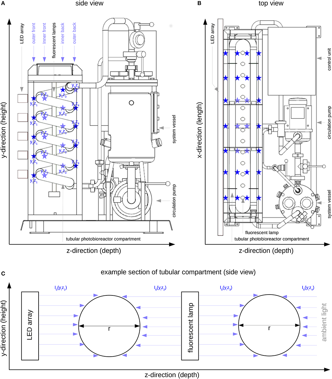
Figure 1. Tubular photobioreactor system PBR30 [IGV Institut für Getreideverarbeitung GmbH, Nuthetal, Germany]; Position of the LED array, the fluorescent lamps and the illuminated tubular reactor part; ⋆ I₀ measuring positions (see also Table 1); (A): Side view; (B): Top view; (C): Representation of four modeled compartments in y/z-direction (referring to Figure 1A), I₀(y_iz_j) - surface light intensity of the respective compartment, y_i - ith position in y-direction, z_j - jth position in z-direction.

The illumination profile of the reactor's tubular glass part was recorded at 140 measuring positions (indicated by ⋆ in Figure 1 and Table 1) at 7 positions in x-direction (width), 5 positions in y-direction (height) and 4 positions in z-direction (depth). All measurements were carried out using the US-SQS described above. Since only minor variations in the light intensities in x-direction were observed (Figure 1B), values in this direction were averaged (see Table 1). The resulting 20 I₀ values refer to their position in y/z-direction as indicated in Figure 1A. These values were used as surface light intensities of the respective reactor compartments within the modeling approach.

TABLE 1

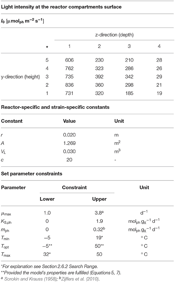
Table 1. Upper part: Light intensity at the reactor surface of the compartments used within the modeling approach, ⋆ Measuring positions (compare Figure 1A); Center part: Reactor-specific and strain-specific constants; Lower part: Set parameter constraints.

The pH value was controlled by the injection of pure CO₂ at the intake side of the circulation pump using a limit controller (set-point pH 7.25; manipulated variable: solenoid-controlled valve; switch-point: pH 7.25; pH hysteresis: 0.05; on-delay: 5 s). The temperature was controlled using a cooling water circuit supplied by a water bath (F12, Julabo GmbH, Seelbach, Germany) and connected to the double jacket of the system vessel (limit comparator; hysteresis: 1 K). The circulation pump frequency was set to 35.7 Hz resulting in a suspension flow velocity of 0.72 m s⁻¹ in the glass tubes.

2.3. Experimental and Modeling Approach

The experimental data used within this work was collected from altogether 15 cultivations which were carried out as a series of discontinuous (batch) bioprocesses in order to avert the lag phase at the start of the individual experiments (see Figure 2). Cultures were harvested partially by draining parts of the suspension and replacing it by fresh, steam sterilized medium (Figure 2). The experiments were designed to be conducted at constant illumination at the reactor surface I₀ but by varying the inoculation biomass concentrations c_X,0, the cultivation cycle times t_cyc and the cultivation temperatures T (see Table 2-lower part and Figures 5A,B). Temperature variations during the cultivations, however, resulted from a limited cooling capacity of the reactor system under strongly differing ambient conditions.

FIGURE 2

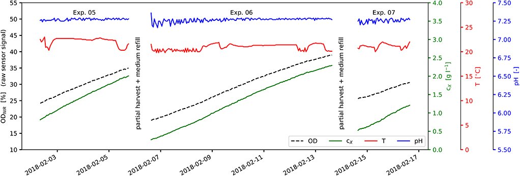
Figure 2. View of experimental process data: Experiments No. 05-07 as part of a series of repeated discontinuous cultivations; experiments are separated by partial harvest and medium refill; OD_NIR, raw sensor signal OD_NIR (black); c_X, correlated biomass concentration (green); T, suspension temperature (red); pH, suspension pH value (blue).

TABLE 2

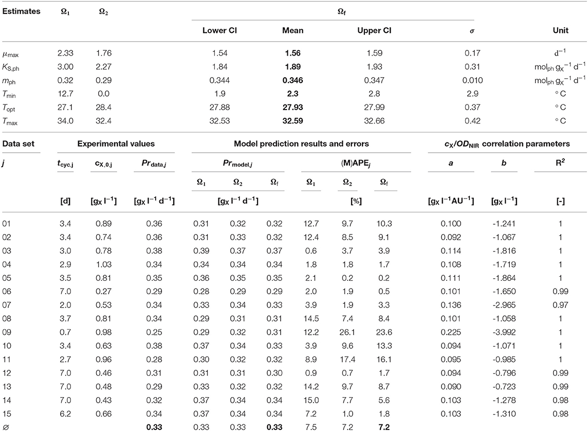
Table 2. Experimental and modeling results: Upper part: Initial Ω₁, Ω₂, and final estimates Ω_f (mean values and jackknife 95 % confidence intervals (CI), if applicable); Lower part: Experimental values and model predictions, c_X/OD_NIR correlation parameters.

In order to carry out the modeling, the photobioreactor was subdivided into 20 glass tube compartments of equal size (z = 1, …, 20). Light intensity at the respective compartment surface was mapped as shown in Table 1 and remained constant during each individual experiment and across the experiments.

As described by Weise et al. (2019), I₀ is considered to be a sum parameter for the light field description at the respective compartment surface. According to Equation (4) only light absorption is taken into account. Due to the actual reactor features (see Figure 1C), the light field is considered to illuminate the compartment y_iz_j from only one side with equal intensity. In addition, because of the particular reactor arrangement, as shown in Figure 1C, each physical compartment is represented by two modeled compartments. The resulting photon fluxes (i.e., light intensity multiplied by surface area) within the modeled compartments were added and then related to the total biomass concentration and the reactor volume (see Equation 4).

2.4. Data Collection

During the experiments a number of variables were determined on-line and off-line. The on-line values of the optical density at near-infrared OD_NIR, the pH and the temperature T were continuously measured and recorded by a 6-channel writer (JUMO Logoscreen 500 cf, Fulda, Germany). The sampling of the off-line values was carried out daily in the morning. The biomass concentration c_X was determined as salt-free dry cell weight. Samples for the dry cell weight determination were homogenized, an aliquot of 10 ml was taken, centrifuged in pre-weighted glass tubes at 4.500 * g for 20 min; the resulting supernatant was discarded and the biomass pellet resuspended in 9 ml deionized water; this washing step was carried out twice. The pellets were dried at 105 °C for 24 h and weighed after cooling in a desiccator for 45 min. Measurements were carried out in duplicate.

The original experimental time series data are available as Supplementary Material.

2.5. Numerical Calculations

All computations were performed using the programming language python (version 3.6.5) and the additional packages astropy (version 3.0.4), numpy (version 1.15.0), pandas (version 0.23.4), SALib (version 1.3.8), scipy (version 1.1.0), and seaborn (version 0.9.0).

2.5.1. Biomass Concentration

c_X [${\mathrm{\text{g}}}_{\text{X}}{\text{l}}^{-1}$] was calculated from on-line OD_NIR [AU] values using a linear correlation. Parameters a [${\text{g}}_{\text{X}}{\text{l}}^{-1}{\text{AU}}^{-1}$] and b [${\text{g}}_{\text{X}}{\text{l}}^{-1}$] (see Table 2-lower part) have been estimated from off-line c_X measurements for each individual experiments (original data not shown).

2.5.2. Averaged Approximated Growth Rate

The calculation of the averaged approximated growth rate ${\bar{\mu }}_{\Delta }$ [d⁻¹] is carried out using the approximation of the ordinary differential equation of the biomass concentration for discontinuous bioprocesses (Equation 8). At first, the approximated growth rate μ_Δ(t) [d⁻¹] is calculated employing the central difference approximation (Equation 9), which is subsequently smoothed using a moving average (Equation 10), where n is the total number of data points i between t − 1 h and t + 1 h. The employed central difference approximation linearizes the growth between the two observations and is therefore only applicable for small Δt (here: Δt = 2 h).

$\begin{array}{ll}\frac{\Delta c_{\text{X}}}{\Delta t}={\mu }_{\Delta }·c_{\text{X}}& (8)\end{array}$

$\begin{array}{ll}{\mu }_{\Delta }(t)=\frac{c_{\text{X}}(t+1\text{h})-c_{\text{X}}(t-1\text{h})}{2\text{h}·c_{\text{X}}(t)}& (9)\end{array}$

$\begin{array}{ll}{\bar{\mu }}_{\Delta }(t)=\frac{1}{n}{\displaystyle \sum _{i_{t-1\text{h}}}^{n=i_{t+1\text{h}}}}{\mu }_{\Delta }(i)& (10)\end{array}$

2.5.3. Biomass Productivity

The experimental biomass productivity for the respective experiment j was calculated as volumetric yield using the following Equation (11) (data point i, i = 0, n).

$\begin{array}{ll}P{r}_j=\frac{c_{\text{X},i=\text{n},j}-c_{\text{X},i=0,j}}{t_{i=\text{n},j}-t_{i=0,j}}& (11)\end{array}$

2.5.4. Model Validation by MAPE

The criterion used to evaluate the model's accuracy was the Mean Absolute Percent Error (MAPE) (Equation 12) (Mayer and Butler, 1993). It is calculated based on measured and modeled productivities considering all experiments (j = 1, …, m). When only a single experiment is considered (m = 1), MAPE is expressed as APE (Absolute Percent Error).

$\begin{array}{ll}\text{MAPE}=\frac{100}{\text{m}}{\displaystyle \sum _{j=1}^m}\left(\frac{|P{r}_{\text{meas},j}-P{r}_{\text{model},j}|}{\left|P{r}_{\text{meas},j}\right|}\right)& (12)\end{array}$

2.6. Parameter Estimation and Model Analysis

In order to parameterize the developed model, a parameter estimation procedure was carried out in two consecutive steps: The initial parameter estimation, following the methodology proposed by Bernard and Rémond (2012), was applied in a first step to generate initial parameter estimates which were then, in a second step, used as starting values for the final parameter estimation. Both stages of the consecutive parameter estimation were carried out using the same experimental (time series) data.

The initial parameter estimation (section 2.6.3) allows to efficiently screen through a wide parameter search range (see section 2.6.2) by fitting the growth kinetics directly to the reorganized data sets (see section 2.6.1). This was carried out in particular with respect to the temperature modeling in order for the unknown cardinal temperatures to converge. Since, however, the reorganization includes approximation and averaging of ${\bar{\mu }}_{\Delta }$ as well as clustering and selection, the returned results are potentially imprecise.

Therefore, the final parameter estimation (section 2.6.4) was carried out by fitting the model output to the original experimental time series data sets, employing the above mentioned initial estimates as starting values.

Based on the model, parameterized this way, the numerical biomass productivity optimization (section 2.6.6) was carried out with respect to the process parameters c_X,0, t_cyc, and T that are to be applied to the process.

2.6.1. Data Set Reorganization

In order to carry out the initial parameter estimation procedure described in the following section, a pooling, reorganization, clustering, and selection of the data was performed:

• Calculating the averaged approximated growth rates ${\bar{\mu }}_{\Delta ,i,j}$ (according to Equation 10) for the i^th data point of the j^th experiment (j = 1, …, 15).

• Concatenating data sets for q_ph,i,j, ${\bar{\mu }}_{\Delta ,i,j}$ and T_i,j from all 15 experiments into a new single data set.

• Reassigning the newly formed entries for ${\bar{\mu }}_{\Delta ,i}$ and T_i that share the same q_ph value to a new k^th data set which corresponds to this particular q_ph value (k = 1, …, s).

• Sorting each data set k obtained by its T_i,k values (for identical T_i,k values, corresponding ${\bar{\mu }}_{\Delta ,i,k}$ values were averaged).

• Clustering the entire q_ph range into 10 equidistant clusters; assigning each data set k to its respective cluster.

• Selecting one data set per q_ph cluster that covers the widest individual T_k range (k = 1, …, 10).

The data sets (k = 1, …, 10) reorganized this way were then applied in the first part of the parameter estimation procedure.

2.6.2. Search Range

An adequate search range for the parameter estimation procedure was determined based on reasonable assumptions. In particular, the temperature range was constrained to -5.0, …, 50.0° C, based on the assumption that growth outside this range is not possible for the genus Nannochloropsis.

• T_min ranges from −5.0°C (lower bound) to the lowest temperature for which experimental data is available (upper bound).

• T_opt ranges from −5.0°C (lower bound) to 50.0 °C (upper bound), as long as the model's properties are fulfilled (see Equations 5, 7).

• T_max ranges from the highest temperature for which experimental data is available (lower bound) to 50.0 °C (upper bound).

• μ_max ranges from the highest ${\bar{\mu }}_{\Delta }$ value obtained from the experiments (lower bound) to the highest μ_max value reported for microalgae (upper bound; see Table 1-lower part).

• K_S,ph ranges from 0 (lower bound) to the highest q_ph value obtained from the experiments (upper bound).

• m_ph ranges from 0 (lower bound) to the highest m_ph value reported in the literature (upper bound; see Table 1-lower part).

2.6.3. Initial Parameter Estimation

Each data set k, reorganized as described above, contains growth rate values ${\bar{\mu }}_{\Delta ,i,k}$ at temperatures T_i,k. Bernard and Rémond (2012) published a strategy that consists in the following: Identifying s + 3 parameters μ_opt,1, μ_opt,2, …, μ_opt,s, T_min, T_opt, T_max (here s = 10, for the 10 cluster data sets) vectorised as θ_T, where the parameter μ_opt,k is the optimum growth rate at the optimum temperature T_opt for the kth data set. Following their strategy, the underlying key assumption is that the cardinal temperatures (T_min, T_opt, T_max) are common to all the data sets, whilst μ_opt,k is constant within the respective data set due to constant experimental lighting conditions q_ph,k. The unknown s + 3 parameter values were estimated in a first step by minimizing the optimization criterion J(θ_T) (Equation 13) (Bernard and Rémond, 2012). Within a second step, the remaining model parameters μ_max, K_S,ph and m_ph (vectorised as θ_qph) were estimated in a similar way (Equation 14). Both, Equations (13) and (14), were minimized with respect to the respective θ resulting in the minimum optimization criterion value J(Ω) for the optimum parameter vector Ω according to Equation (15).

$\begin{array}{ll}J({\theta }_T)={\displaystyle \sum _{k=1}^s}{\displaystyle \sum _{i=1}^n}{\left({\bar{\mu }}_{\Delta ,i,k}-{\mu }_{\text{opt},k}·\varphi (T_{i,k},T_{\text{min}},T_{\text{opt}},T_{\text{max}})\right)}^2& (13)\end{array}$

$\begin{array}{ll}J({\theta }_{q_{\text{ph}}})={\displaystyle \sum _{k=1}^s}{\left({\mu }_{\text{opt},k}-{\mu }_{\text{opt}}(q_{\text{ph},k},{\mu }_{\text{max}},K_{\text{S,ph}},m_{\text{ph}}){|}_{T_{\text{opt}}}\right)}^2& (14)\end{array}$

$\begin{array}{ll}J(\Omega )={\displaystyle \underset{\theta }{\text{min}}}J(\theta )& (15)\end{array}$

The downhill-simplex method (Nelder-Mead method) used for the model parameter estimation procedure (scipy.optimize.fmin) was started from every possible parameter value combination within the search ranges described above. The T range was screened stepwise by ΔT = 5 °C, resulting in 70 initializations that match the model's properties (Equations 5, 7). The ranges for μ_max, K_S,ph and m_ph were screened using 10 equidistant values along each axis, resulting in 1,000 initializations. The method was set to perform a maximum of 200 iterations for each initialization. Computations were carried out using the standard settings of the above package regarding the convergence criteria of the method.

2.6.4. Final Parameter Estimation

Since the initial parameter estimation described above can provide results which are potentially imprecise due to the approximation and averaging of ${\bar{\mu }}_{\Delta }$, the reorganization and clustering of the data sets k as well as the split parameter estimation of θ_T and θ_qph, a second and final parameter estimation step was carried out. Based on the ordinary differential equation of the biomass concentration for discontinuous bioprocesses (Equation 16), the original experimental time series data sets j (j = 1, …, 15) were simulated using the initial parameter estimates. Numerical integration was carried out employing the Euler method. The time series of c_X were simulated for the i discrete time points t_i,j and their corresponding temperatures T_i,j.

$\begin{array}{ll}\frac{d{c}_{\text{X}}}{dt}=\mu (q_{\text{ph}},T)·c_{\text{X}}& (16)\end{array}$

The objective of this final parameter estimation was to identify the m + 6 parameters c_X,0,1, c_X,0,2,…, c_X,0,m, μ_max, K_S,ph, m_ph, T_min, T_opt, T_max (here m = 15, for the 15 experiments) vectorised as θ_f, where the parameter c_X,0,j is the inoculation biomass concentration c_X,0 for the jth data set. The optimum parameter values were estimated by minimizing the optimization criterion J(θ_f) (Equation 17). The final optimum parameter vector Ω_f (according to Equation 18) was determined in analogy to the initial parameter estimation as described above.

$\begin{array}{ll}J({\theta }_{\text{f}})={\displaystyle \sum _{j=1}^m}{\displaystyle \sum _{i=1}^n}{(c_{\text{X,meas}}-c_{\text{X,pred}})}^2& (17)\end{array}$

with

$\begin{array}{l}{c}_{\text{X},\text{meas}}=c_{\text{X},\text{data},i,j}\hfill \\ c_{\text{X},\text{pred}}=c_{\text{X},\text{model},i,j}(q_{\text{ph},i,j},T_{i,j},c_{\text{X},0,j},{\mu }_{\text{max}},K_{\text{S},\text{ph}},m_{\text{ph}},T_{\text{min}},\hfill \\ T_{opt},T_{\max })\hfill \\ J({\Omega }_{\text{f}})={\displaystyle \underset{\theta }{\text{min}}}J({\theta }_{\text{f}})& (18)\end{array}$

The Nelder-Mead method was also employed for this second step of the model parameter estimation procedure (scipy.optimize.fmin). The initially estimated parameter vectors were now used as start parameter vectors. The method was set to carry out a maximum of 200 iterations for each initialization. Again, the standard settings of the above package were used with respect to the convergence criteria.

Since the values of the parameters T_min and T_max to be estimated were expected to lie outside the experimental data range and to account for the relatively small number of experiments, the Delete-2-Jackknife analysis (astropy.stats.jackknife_stats) was used to indicate the 95 % confidence interval of the identified parameters of the vector Ω_f (Efron and Tibshirani, 1993; Duchesne and MacGregor, 2001). Jackknife re-sampling was carried out by bootstrapping two respective data sets (experiments) from the data at a time.

2.6.5. Parameter Sensitivity Analysis

A variance-based sensitivity analysis according to Sobol (2001) was performed using the SALib.analyze.sobol in order to investigate the model's parameter sensitivities more deeply. This sensitivity analysis was done with respect to the biomass productivity as the main focus of this study. Within Equation (19), M represents the model output depending on the process parameters c_X,0, t_cyc and T as well as the model parameter vector θ (Zhang et al., 2017) consisting of μ_max, K_S,ph, m_ph, T_min, T_opt, and T_max.

The Sobol method is based on the decomposition of the variance of the model output Var(M) (Equation 20) into summands of increasing dimensionality (Zhang et al., 2015, 2017). Var_i is the partial variance corresponding to the first-order index of θ_i of the model output M, while Var_ij is the partial variance corresponding to the second-order index of the ith and jth parameter interaction (Zhang et al., 2015, 2017). k is the number of model parameters, here k = 6.

$\begin{array}{ll}M=P{r}_{\text{model}}(c_{\text{X},0},t_{\text{cyc}},T,\theta )& (19)\end{array}$

$\begin{array}{ll}Var(M)={\displaystyle \sum _{i=1}^k}Va{r}_i+{\displaystyle \sum _{i=1}^{k-1}}{\displaystyle \sum _{j=i+1}^k}Va{r}_{ij}+\dots +Va{r}_{1,\dots ,k}& (20)\end{array}$

The sensitivity indices S_i and S_ij (Equations 21, 22) are calculated as ratios of the partial variances to the total variance (Zhang et al., 2015). Total-order indices S_Ti are calculated following Equation (23) using Var_~i which represents the variation of all parameters except θ_i (Homma and Saltelli, 1996; Sobol, 2001; Zhang et al., 2017). S_i quantifies the effect of varying θ_i alone, while S_Ti quantifies the effect of varying θ_i and includes all effects caused by its interactions with all other model parameters.

$\begin{array}{ll}\text{First-order index }{S}_i=\frac{Va{r}_i}{Var}& (21)\end{array}$

$\begin{array}{ll}\text{Second-order index }{S}_{ij}=\frac{Va{r}_{ij}}{Var}& (22)\end{array}$

$\begin{array}{ll}\text{Total-order index }{S}_{Ti}=S_i+{\displaystyle \sum _{j\ne i}}{S}_{ij}+\dots =1-\frac{Va{r}_{~i}}{Var}& (23)\end{array}$

The Saltelli sampling scheme (SALib.sample.saltelli) was used to generate model parameter samples of the final model parameter estimates Ω_f (section 2.6.4) varied by ±3σ (see Table 2-upper part). This scheme generates N · (2k + 2) samples (here N = 10,000; k = 5). The calculated indices were classified using thresholds. Indices contributing <0.01 to the model output variance are considered “non-sensitive,” while indices contributing ≥ 0.1 are considered “highly sensitive” (Tang et al., 2007).

S_i and S_Ti also potentially depend on the process parameters. The experimentally set c_X,0 is associated with the present light availability, while the set T may influence the sensitivity of the three cardinal temperatures. Therefore, the sensitivity analysis was carried out for 9 combinations (scenarios) of c_X,0 and T taking into account data corresponding to percentages of the respective experimental range [20% (“low”), 50% (“medium”), and 80% (“high”)].

2.6.6. Biomass Productivity Optimization

In order to optimize the biomass productivity Pr with respect to the described photobioreactor, a numerical optimization was carried out. The objective was to maximize Pr with respect to the process parameters c_X,0, t_cyc, and T. Numerical integration of Equation (16) was performed using the estimated model parameters (Ω_f; Table 2-upper part) by employing lsoda of the ODEPACK (scipy.integrate.odeint). After each integration, Pr was calculated for the individual iteration steps using Equation (11). The process parameters c_X,0, t_cyc, and T were vectorised as θ_Pr containing all possible process parameter combinations, while Ω_Pr contains the optimum process parameter combination with respect to Pr. The optimum process parameter values were estimated by minimizing the optimization criterion J(θ_Pr) (Equations 24, 25) using also the downhill-simplex method (Nelder-Mead method; scipy.optimize.fmin). With respect to numerical integration and convergence criteria, standard settings of the above packages were used.

$\begin{array}{ll}J({\theta }_{\text{Pr}})=-P{r}_{\text{model}}(c_{\text{X},0},t_{\text{cyc}},T)& (24)\end{array}$

$\begin{array}{ll}J({\Omega }_{\text{Pr}})={\displaystyle \underset{\theta }{\text{min}}}J({\theta }_{\text{Pr}})& (25)\end{array}$

3. Results and Discussion

The experiments carried out and presented here consisted of a series of discontinuous (batch) cultivations. Single experiments were separated by partial harvest of the biomass suspension and replacement by new medium (see Figure 2). Inoculation biomass concentrations c_X,0 and cultivation cycle times t_cyc were varied between the experiments (see Figure 2 and Table 2-lower part). Temperature T as well as pH were recorded during the experiments (see Figures 2, 5A,B). The original experimental time series data and the reorganized data sets are available as Supplementary Material.

Light saturation was not observed during the experiments. The linear accumulation of biomass indicates limited lighting conditions (Figure 2). The light intensity at the photobioreactor surface varied between 19 and 836 $\mu {\text{mol}}_{\text{ph}}{\text{m}}^{-2}{\text{s}}^{-1}$ (average: 337 $\mu {\text{mol}}_{\text{ph}}{\text{m}}^{-2}{\text{s}}^{-1}$; see Table 1-upper part and Figure 1). These incident light intensities range from low values (100 $\mu {\text{mol}}_{\text{ph}}{\text{m}}^{-2}{\text{s}}^{-1}$ Raso et al., 2011) to rather typical values at lab-scale (700 $\mu {\text{mol}}_{\text{ph}}{\text{m}}^{-2}{\text{s}}^{-1}$ Pal et al., 2011; up to 850 $\mu {\text{mol}}_{\text{ph}}{\text{m}}^{-2}{\text{s}}^{-1}$ Wagenen et al., 2012) for Nannochloropsis sp. With respect to the scalability toward outdoor production, higher incident light intensities of 1,500 to 2,000 $\mu {\text{mol}}_{\text{ph}}{\text{m}}^{-2}{\text{s}}^{-1}$ are present on sunny days. These however are lowered due to the vertical arrangement of the glass tubes at industrial scale, the light absorption by greenhouse parts, etc. Therefore, the comparability and the transferability of presented model to industrial-scale outdoor conditions is limited unless further model extensions regarding higher variability in light and temperature, nightly biomass losses, etc. are carried out.

The inoculation biomass concentrations within this study (0.27,…, 1.03 ${\text{g}}_{\text{X}}{\text{l}}^{-1}$) are within a typical range for both, lab-scale and outdoor production of Nannochloropsis sp. in tubular photobioreactors (Olofsson et al., 2012; Pfaffinger et al., 2016; Pereira et al., 2018). The experimental variability regarding c_X,0 is rather high within the investigated small pilot-scale experiments. However, biomass concentrations throughout the cultivation cycle time are found to be typical for large-scale and outdoor production of Nannochloropsis. c_X ranged 0.27,…, 2.79 ${\text{g}}_{\text{X}}{\text{l}}^{-1}$, reflecting usual inoculation and harvesting biomass concentrations, respectively. To the best of our knowledge, depending on the climatic zone, biomass concentrations of Nannochloropsis outdoor cultures within tubular photobioreactors rarely exceed 3 ${\text{g}}_{\text{X}}{\text{l}}^{-1}$ (Olofsson et al., 2012; Benvenuti et al., 2015) and do not exceed 5 ${\text{g}}_{\text{X}}{\text{l}}^{-1}$ (Zittelli et al., 1999). Therefore, the c_X range observed here is comparable to larger-scale and outdoor processes.

Biomass productivity Pr was calculated for each experiment according to Equation (11) in order to evaluate the model's accuracy expressed as MAPE (see Table 2-lower part) and to use it for the biomass productivity optimization. The overall context of this work was to optimize Pr as part of a series of batch bioprocesses (i.e., repeated batch).

The devised two-stage consecutive parameter estimation procedure was carried out using the reactor-specific and strain-specific constants as well as the set parameter constraints shown in Table 1.

The initial parameter estimation converged to two valid solutions (Ω₁ and Ω₂, Table 2-upper part) depending on the start parameter combinations. Both solutions differ only strongly in the estimated value of T_min.

Both initial parameter estimation vectors (Ω₁ and Ω₂) were used as start parameter combinations for the final parameter estimation. It was performed using the original time series data sets j (in contrast to the reorganized data sets k). The altogether six shared model parameters where estimated within multi-experiment fittings.

The final parameter estimation converged to the solution Ω_f (Table 2-upper part, Figure 3) initialized from each of the two initial parameter combinations (Ω₁ and Ω₂). The ϕ(T) data shown in Figure 3A was normalized with respect to the corresponding estimated μ_opt (Figure 3B) according to Equation (1).

FIGURE 3

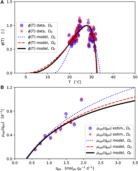
Figure 3. Model parameter estimation results: Initial parameter estimation provides solutions Ω₁ and Ω₂ and final parameter estimation solution Ω_f (see Table 2–upper part); (A): CTMI estimation ϕ(T) vs. T (Equations 5–7); (B): Estimation μ_opt(q_ph) vs. q_ph (Equation 2).

The estimated values of T_min and T_max lie outside the range 19, …, 31 °C of available experimental data. Since the range between the estimated T_min and the available data is much wider than the one between the estimated T_max and the available data, in particular the T_min estimation is afflicted with some uncertainty, which is further enforced by the asymmetric shape of the temperature function ϕ(T) as can be seen in Figure 3A showing the CTMI results. This is underlined by the jackknife 95 % confidence intervals CI and standard deviations σ of the estimated parameters (Table 2-upper part). While for all other parameters the σ values indicate relatively certain parameter estimations, σ for T_min is at the same order of magnitude as the parameter's value.

The finally estimated cardinal temperatures for N. granulata (T_min = 2.3°C, T_opt = 27.93°C, T_max = 32.59°C) lie within the specified parameter constraint ranges (Table 1) and match laboratory experience. The CTMI parameters estimated by Bernard and Rémond (2012) for the related species N. oceanica (data by Sandnes et al., 2005) showing a good degree of similarity (T_min = −0.2°C, T_opt = 26.7 °C, T_max = 33.3 °C).

The results obtained here are supported by an optimum growth temperature range of 20, …, 29 °C given in the literature (Sukenik, 1991; Wagenen et al., 2012; Bartley et al., 2015; Abirami et al., 2017). Further, Wagenen et al. (2012) reported only very poor growth below 13.6 °C and above 32.3°C for N. salina. Also, Sukenik (1991) found that Nannochloropsis spp. failed to grow below 10 °C and above 38 °C. In view of the fact that the parameter estimation carried out here had only rough quantitative specifications with regard to the cardinal temperatures, the values calculated (Table 2-upper part) are in strong compliance with the literature. Sandnes et al. (2005) empirically described a light-dependent optimum cardinal temperature T_opt for N. oceania (Sandnes et al., 2005). Although this combined effect of light and temperature is physiologically plausible, the functional relationship of these two variables was not observed for N. granulata within the own data.

The μ_opt values for Ω₁ and Ω₂ estimated increase monotonically with higher q_ph (Figure 3B). These estimates are subject to fluctuations but show no inhibition within the observed q_ph range. Therefore, a growth kinetics considering light limitation (Equation 2) without light inhibition was applied. The q_ph range observed during the experiments (0.59, …, 1.9 ${\text{mol}}_{\text{ph}}{{\text{g}}_{\text{X}}}^{-1}{\text{d}}^{-1}$) is comparable to q_ph values given by the literature (0.25, …, 2.2 ${\text{mol}}_{\text{ph}}{{\text{g}}_{\text{X}}}^{-1}{\text{d}}^{-1}$) (Zijffers et al., 2010; Kandilian et al., 2014; Janssen et al., 2018). In accordance with Equation (4) q_ph is calculated as a mean light availability rate of the whole culture suspension, considering the total culture volume V_L. However, local light intensities differ due to light gradients within the culture suspension, which are not spatially resolved within the model. Despite this aggregation, the devised model predicts microalgal growth and biomass productivities precisely. The estimated photon maintenance coefficient m_ph = 0.346 ${\text{mol}}_{\text{ph}}{{\text{g}}_{\text{X}}}^{-1}{\text{d}}^{-1}$ is comparable to values reported for C. sorokiniana: 0.16 ${\text{mol}}_{\text{ph}}{{\text{g}}_{\text{X}}}^{-1}{\text{d}}^{-1}$ and D. tertiolecta: 0.32 ${\text{mol}}_{\text{ph}}{{\text{g}}_{\text{X}}}^{-1}{\text{d}}^{-1}$ (Zijffers et al., 2010). Pirt (1986) reported increasing m_ph values for photobioreactor set-ups with lower illuminated/non-illuminated culture volume ratios, which has to be considered during the transfer to different photobioreactor set-ups. The growth yield Y_X,ph [${\text{g}}_{\text{X}}{{\text{mol}}_{\text{ph}}}^{-1}$], calculated following, Pirt (1986) as Y_X,ph = μ_opt / (q_ph − m_ph), varied 0.45, …, 0.73 ${\text{g}}_{\text{X}}{{\text{mol}}_{\text{ph}}}^{-1}$ during the experiments (based on Figure 3B), which matches the Y_X,ph range of 0.2, …, 2.1 ${\text{g}}_{\text{X}}{{\text{mol}}_{\text{ph}}}^{-1}$ reported in the literature (Zijffers et al., 2010; Dillschneider et al., 2013; Schediwy et al., 2019). The estimated parameter μ_max = 1.56 d⁻¹ is comparable also to μ_max ranges between 0.86, …, 1.6 d⁻¹ as found in the literature (Sandnes et al., 2005; Spolaore et al., 2006; Weise et al., 2019).

The similar parameters indicate that the model structure in particular with respect to the light-limited growth modeling shows a good transferability for tubular photobioreactors that differ in scale, glass tube diameter and the mode of bioprocess operation, although the experimental and modeling approaches differed in many respects. In contrast to Weise et al. (2019), who considered constant temperature conditions (T = 22 °C) under steady-state turbidostatic bioprocess operation, experiments presented here were conducted under variable temperature conditions and have been scaled up by ≈ 7x regarding the reactor liquid volume V_L, by 10x regarding the number of modeled compartments and by 2x regarding the glass tube diameter.

In order to transfer the devised model to other reactors and different scales, it is necessary to consider homogeneous one-sided illuminated glass tube compartments within the model, although the glass tubes may be illuminated homogeneously from both sides in the actual arrangement. Therefore in this context also, the physical compartments are to be decomposed mathematically into several theoretical ones. If these assumptions do not apply to the specific photobioreactor structure, the model cannot be transferred without further modification. The presented model considers basic geometric properties (e.g., inner tube radius, liquid reactor volume, illuminated reactor surface, etc.) of tubular photobioreactors. Using biomass productivity or reactor size as scale-up objectives, it is possible to estimate the dimensions (e. g. illuminated reactor surface) of a photobioreactor scale-up.

The presented model is implemented using the ordinary differential equation (ODE) for batch bioprocesses. In order to adapt the model for continuous cultivation, the ODE for batch bioprocesses can be extended by a dilution term. The growth kinetics, which are described by algebraic equations are not affected by this extension.

With respect to the model's sensitivity analysis, Figure 4 illustrates the first-order and total-order sensitivity indices of the model parameters across different scenarios. The comparatively small differences in the values of S_i and S_Ti indicate only limited interactions between the parameters, which was to be expected due to the model's structure (see Equations 1, 2, 7). The output of the model is highly sensitive (S_i and S_Ti ≥ 0.1) with respect to the parameters μ_max and K_S,ph. Both parameters combined contribute predominantly to the variance in the model output, since they describe the utilization of light as the sole energy source for phototrophic growth. The set c_X,0 effects the sensitivities of K_S,ph and m_ph. Since higher c_X,0 reduce the q_ph, the photon half-saturation constant K_S,ph becomes more sensitive. In addition, m_ph becomes sensitive (S_i and S_Ti ≥ 0.01) only at higher c_X,0 (Figure 4).

FIGURE 4

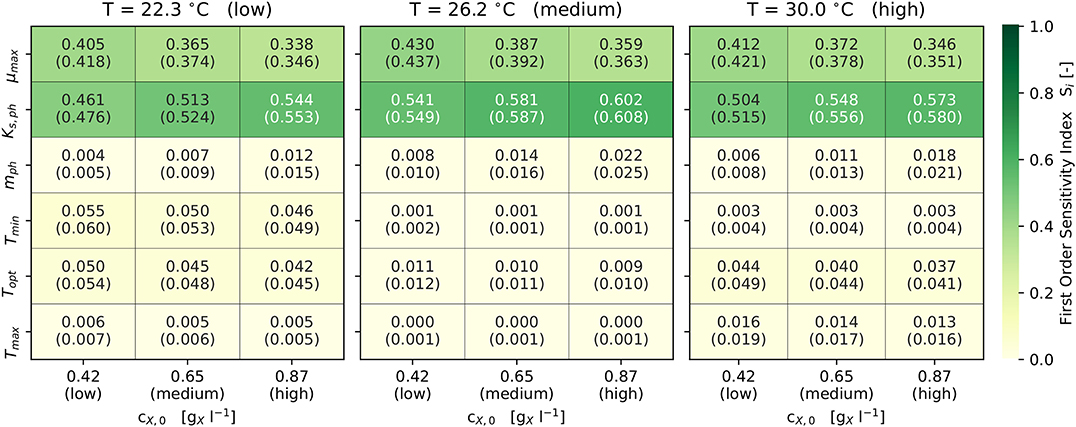
Figure 4. Results of the Sobol sensitivity analysis: First and (total) order sensitivity indices for Ω_f ± 3σ and 9 scenarios (3 each for c_X,0 and T).

T_opt is sensitive (S_i and S_Ti ≥ 0.01) in all scenarios, while T_min and T_max are sensitive only at lower and higher temperatures. Also, T_min and T_max become non-sensitive at temperatures close to T_opt. At temperatures away from T_opt, the combined sensitivity of the three cardinal temperatures contributes up to 10 % (i.e., 0.1) to the model's output variance. The set c_X,0 does not influence the sensitivity of the cardinal temperatures.

All experiments were carried out in the range 20, …, 25°C, except Experiment No. 10 at 31°C. Although the temperature inside the photobioreactor was actively controlled, diurnal rhythms in the ambient temperature resulted in temperature variations within individual experiments. These are displayed in Figure 5A using kernel density approximations (violins). The width of the individual violin represents the number of available data at the respective temperature value, while small pin-like tails of the violins indicate short-term outliers of the measured variable. In analogy, Figure 5B shows the distribution of the measured pH values of the respective experiments. Variations in temperature and pH value did not occur rapidly, as can be seen in Figure 2. Despite the variations in the observed temperature and pH ranges, using the specific approach applied here, the available data could be successfully processed in order to estimate model parameters and optimize process parameters at pilot-scale. Figure 5C provides violin plots that represent the absolute modeling error with respect to the biomass concentration time series using the estimated parameter vector Ω_f. It can be seen that the modeling error rarely exceeds ± 0.15 ${\text{g}}_{\text{X}}{\text{l}}^{-1}$.

FIGURE 5

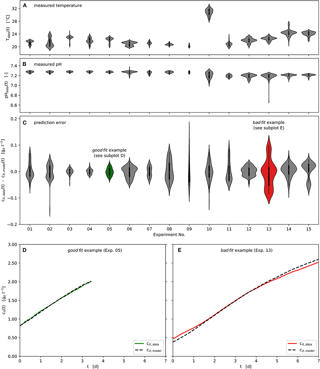
Figure 5. Experimental and modeling results: Time series of measured and modeled biomass concentration, measured temperature and pH; Violin plots: center point - median, box - interquartile range (IQR), whisker - 1.5 · IQR, kernel density estimation - number of observations; (A): Temperature distributions of the experimental time series data; (B): pH distributions of the experimental time series data; (C): Model prediction error distributions of the experimental time series data with respect to biomass concentration; (D): “good fit” example - representing lowest prediction error calculated, Experiment No. 05; (E): “bad fit” example - representing highest prediction error calculated, Experiment No. 13.

Furthermore, one good as well as one badly predicted experiment are highlighted in green (Experiment No. 05) and red (Experiment No. 13), as shown in Figure 5C. These two experiments are presented as time series in Figures 5D,E. Although the biomass concentration has been well predicted over much of the time (Figures 5D,E), some regions are underestimated or overestimated at the beginning and the end of the respective experiments (Figure 5E as example).

The prediction accuracy MAPE (Equation 12) of the target value biomass productivity Pr (Equation 11) improved over the course of the estimation procedures. Table 2-lower part provides an overview of these experimental and modeling results as well as the parameters a and b. The initial parameter estimation of Ω₁ and Ω₂ resulted in MAPE(Ω₁) = 7.5% and MAPE(Ω₂) = 7.2%, whilst the prediction accuracy after the final parameter estimation was MAPE(Ω_f) = 7.2%. Therefore, the accomplished overall model prediction accuracy is very satisfactory, although the Absolute Percent Error of individual experiments (APE_j) covers a wider range 0.1, …, 26.1%. Typical MAPE values for industrial and business data and their interpretation are: < 10% highly accurate forecasting, 10, …, 20% good forecasting, 20, …, 50% reasonable forecasting, > 50% inaccurate forecasting (Lewis, 1982; Moreno et al., 2013).

Based on the results of the parameter estimation procedure (Table 2-upper part), the parameterized model has been used to design an optimized bioprocess regime regarding the inoculation biomass concentration c_X,0, the cultivation cycle time t_cyc and the temperature T with respect to optimum biomass productivity Pr_opt for a series of equal batch cultivations (repeated batches). Since, the specific light availability rate q_ph decreases monotonously along with biomass accumulation under constantly illuminated discontinuous bioprocess operation, q_ph is only influenced by alterable c_X,0 and t_cyc.

Following the above objective, a numerical optimization of Pr was conducted using Equations (24) and (25) as described in section 2.6.6. The biomass productivity optimization showed two major aspects: First, the optimum growth temperature equals the model parameter T_opt = 27.93°C, which matches the intuitive expectation with regard to Equations (1) and (5). This applies independently of the lighting conditions according to the devised model. Second, the optimization results in a corner point optimum that points toward an insignificantly small cultivation cycle time t_cyc → 0.

The developed approach therefore predicts the theoretical optimum biomass productivity Pr_opt → 0.50 ${\text{g}}_{\text{X}}{\text{l}}^{-1}{\text{d}}^{-1}$ within the investigated bioreactor set-up for negligibly small cultivation cycle times with c_X,0,opt → 1.07 ${\text{g}}_{\text{X}}{\text{l}}^{-1}$, and hence the transition from discontinuous (e.g., batch, fed-batch or their repeated versions) to continuous (e.g., chemostat, turbidostat) bioprocess operation. The optimum inoculation biomass concentration c_X,0,opt calculated this way corresponds to the steady-state biomass concentration of a settled chemostat bioprocess or to the optimum biomass concentration set-point of a turbidostat bioprocess, respectively (Weise et al., 2019). (Statement is no longer applicable due to the modifiaction of Equation 2). The above findings are also supported by Chen et al. (2012) who estimated c_X,0,opt = 0.98 ${\text{g}}_{\text{X}}{\text{l}}^{-1}$ (Pr_opt = 0.75 ${\text{g}}_{\text{X}}{\text{l}}^{-1}{\text{d}}^{-1}$) for a small-scale laboratory set-up, as well as Hulatt et al. (2017) finding Pr_opt = 0.51 ${\text{g}}_{\text{X}}{\text{l}}^{-1}{\text{d}}^{-1}$ for a flat-panel photobioreactor, both under discontinuous operation. In addition, literature values for Pr at pilot-scale and industrial-scale show a range <0.1, …, 0.71 ${\text{g}}_{\text{X}}{\text{l}}^{-1}{\text{d}}^{-1}$ (de Vree et al., 2015; Pereira et al., 2018), confirming the feasibility of the Pr_opt values obtained here.

A simulation of the original experiments was carried out using the actually applied cultivation cycles times t_cyc of the experiments (see Table 2-lower part) as well as the optimized process parameters c_X,0,opt and T_opt (according to section 2.6.6). The model predicts a noticeable increase of Pr by 39% from 0.33 ${\text{g}}_{\text{X}}{\text{l}}^{-1}{\text{d}}^{-1}$ (see Table 2-lower part) to 0.46 ${\text{g}}_{\text{X}}{\text{l}}^{-1}{\text{d}}^{-1}$.

The convergence toward the predicted optimum biomass productivity is asymptotic. This results in only minor additional gains in biomass productivity when moving from short-cycled discontinuous to continuous bioprocesses and requires a simultaneous adaptation of the inoculation biomass concentration c_X,0. Within this context, Table 3 shows examples of the predicted Pr_opt under discontinuous (repeated batch) bioprocess operation for fixed cultivation cycle times t_cyc (1 d, 3.5 d, and 7 d) starting at the required inoculation biomass concentration c_X,0 and under optimum temperature T_opt. As a consequence, solely reducing t_cyc from 7 d to 3.5 d would outweigh the increase in operational efforts by a higher Pr (0.37 → 0.46 ${\text{g}}_{\text{X}}{\text{l}}^{-1}{\text{d}}^{-1}$; with c_X,0,opt 0.17 → 0.43 ${\text{g}}_{\text{X}}{\text{l}}^{-1}$) under discontinuous bioprocess operation.

TABLE 3

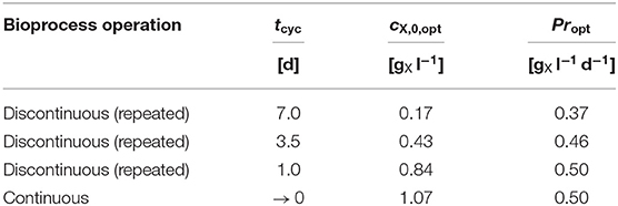
Table 3. Numerical optimization results: Model predicted Pr_opt for different bioprocess operations and pre-set t_cyc at T_opt with the required c_X,0,opt (see Figure 6A).

Figure 6A illustrates these relations in more detail by presenting the model's prediction with respect to biomass productivity Pr depending on the cultivation cycle time t_cyc and the inoculation biomass concentration c_X,0 for the optimum cultivation temperature T_opt. According to the model's prediction, only moderately high biomass productivities are gained for cultivation cycle times greater ≈ 5 days, as well as for inoculation biomass concentrations above ≈ 1 ${\text{g}}_{\text{X}}{\text{l}}^{-1}$ (Figure 6A). Notably, the optimum productivity is reached at the shortest cultivation cycle time, which illustrates the said corner point optimum regarding the cultivation cycle time t_cyc.

FIGURE 6

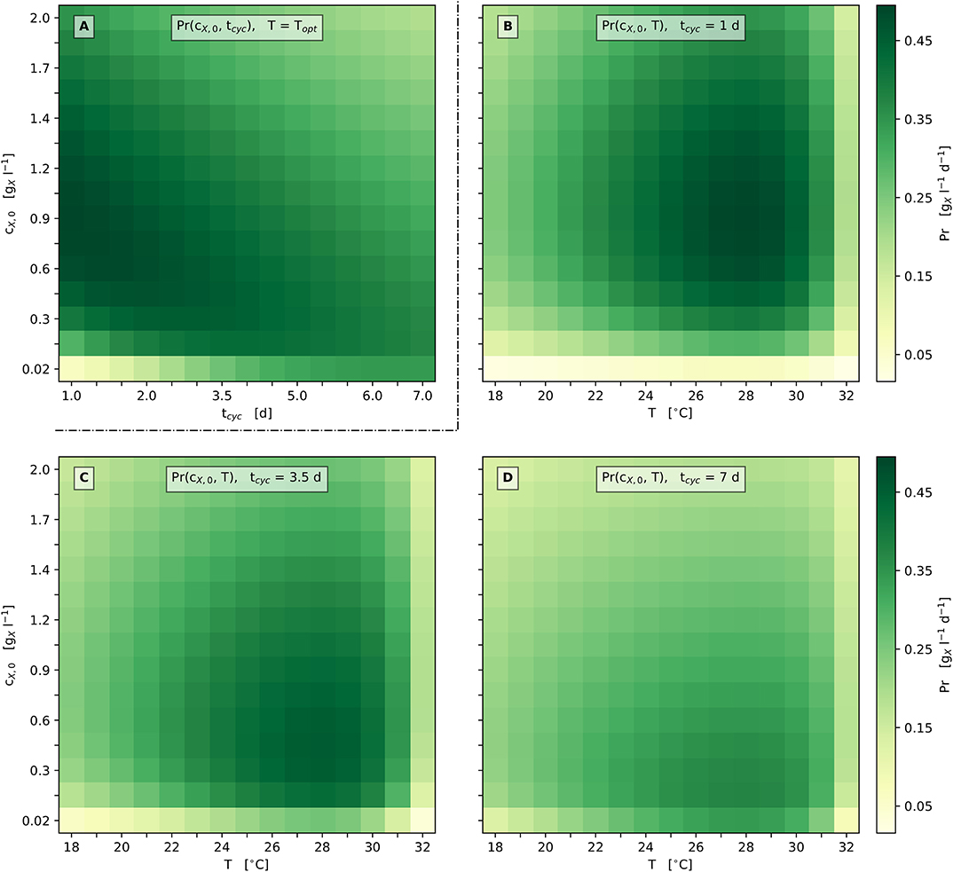
Figure 6. Heat map representation of model predicted biomass productivity; (A): Pr depending on t_cyc and c_X,0 at T_opt; (B–D): Pr depending on T and c_X,0 at set t_cyc [1 d (B), 3.5 d (C), 7 d (D)].

In accordance with these findings, Figures 6B–D additionally provides graphical representations of the biomass productivity loss when varying the process parameters c_X,0, t_cyc and T. Figures 6B–D illustrate scenarios for three different cultivation cycle times: 1 d, 3.5 d (1/2 week), and 7 d (1 week) with respect to discontinuous bioprocess operation (repeated batch). Considerations regarding lag phases are neglected here, as can be seen in Figures 2, 5D,E. All three scenarios show a single optimum of biomass productivity at the respective optimum temperature T_opt and the optimum inoculation biomass concentration c_X,0,opt.

The predicted Pr_opt increases by about 35% from 0.37 ${\text{g}}_{\text{X}}{\text{l}}^{-1}{\text{d}}^{-1}$ at t_cyc = 7 d (c_X,0,opt = 0.17 ${\text{g}}_{\text{X}}{\text{l}}^{-1}$) to 0.50 ${\text{g}}_{\text{X}}{\text{l}}^{-1}{\text{d}}^{-1}$ at t_cyc = 1 d (c_X,0,opt = 0.84 ${\text{g}}_{\text{X}}{\text{l}}^{-1}$). In general, the optimum biomass productivity Pr_opt increases when the cultivation cycle time is shortened. In addition, when this time is shortened, a higher c_X,0,opt is required to obtain the optimum productivity.

4. Conclusion

The work presented here provides a transferable methodology to model microalgal growth covering light availability and temperature based on experimental data from cultivation runs in a small pilot-scale tubular photobioreactor under discontinuous operation in order to subject it to biomass productivity analysis and optimization.

The established model with its estimated parameters accurately predicts light and temperature dependent growth of Nannochloropsis granulata. The parameter ranges are supported by the literature. In general, the model parameter T_opt is much closer to T_max than to T_min, thus the CTMI displays a strong asymmetry. Temperatures above T_opt therefore lead to a steep decline in the growth rate and also the biomass productivity. Since an accurate temperature control is hardly to provide under large-scale or outdoor conditions, these processes should be operated below the targeted T_opt.

Model-based numerical biomass productivity optimization for repeated discontinuous operation points toward best performance under continuous operation. The optimization for repeated discontinuous operation yields reduction of cultivation cycle time and increase of inoculation biomass at optimum temperature. The calculated optimum inoculation biomass concentrations c_X,0,opt and the corresponding optimum biomass productivities Pr_opt are confirmed by different publications. Furthermore, biomass productivities for laboratory-scale, pilot-scale and industrial-scale reported in the literature support the feasibility of the Pr_opt values obtained here. Applying these optimized process parameters would deliver a noticeable increase in biomass productivity.

The successful application of this approach here to small pilot-scale under discontinuous operation, following a previous investigation into lab-scale under continuous operation, indicates its potential transferability also to larger scale tubular photobioreactors covering both light and temperature dependent microalgal growth and biomass productivity.

Data Availability Statement

All datasets generated for this study are included in the article/Supplementary Material.

Author Contributions

TW contributed to the conception and design of the study, the collection and assembly of data, the analysis and interpretation of the data, the drafting, critical revision and final approval of the article. CG contributed to the collection and assembly of data, the drafting, critical revision and final approval of the article and to obtaining funding. MP contributed to the conception and design of the study, the interpretation of the data, the drafting, critical revision and final approval of the article and to obtaining funding.

Funding

The authors gratefully acknowledge the financial support of this work by the Free State of Thuringia, Germany, and the European Union within the project nos. 2015 FE 9151, 2015 FE 9149, EFRE-OP 2014-2020. Additional financial support was provided by the University of Applied Sciences Jena.

Conflict of Interest

TW is collaborative doctoral candidate at the University of Applied Sciences Jena, Jena, Germany and the Friedrich Schiller University Jena, Jena, Germany. TW was employed by the University of Applied Sciences Jena, Jena, Germany and is now employed by the company BioControl Jena GmbH, Jena, Germany. CG is employed by the company Salata AG, Ritschenhausen, Germany. MP is professor at the University of Applied Sciences Jena, Jena, Germany. MP owns stock in the company BioControl Jena GmbH, Jena, Germany.

Acknowledgments

The technical assistance in culturing by G. Pogge (Salata AG, Ritschenhausen) is gratefully acknowledged. Further, the authors thank S. Henkel and D. Driesch (project partner BioControl Jena GmbH) as well as J. Demmel and J. M. Reinecke (University of Applied Sciences Jena, Department of Medical Engineering and Biotechnology) for very helpful discussions with respect to data analysis issues and also S. Schuster (Friedrich Schiller University Jena, Department of Bioinformatics) for assistance with respect to modeling issues.

Supplementary Material

The Supplementary Material for this article can be found online at: https://www.frontiersin.org/articles/10.3389/fbioe.2020.00453/full#supplementary-material

References

Abirami, S., Murugesan, S., Sivamurugan, V., and Sivaswamy, S. N. (2017). Screening and optimization of culture conditions of Nannochloropsis gaditana for omega 3 fatty acid production. J. Appl. Biol. Biotechnol. 5, 13–17. doi: 10.7324/JABB.2017.50303

CrossRef Full Text | Google Scholar

Barbera, E., Grandi, A., Borella, L., Bertucco, A., and Sforza, E. (2019). Continuous cultivation as a method to assess the maximum specific growth rate of photosynthetic organisms. Front. Bioeng. Biotechnol. 7:274. doi: 10.3389/fbioe.2019.00274

PubMed Abstract | CrossRef Full Text | Google Scholar

Bartley, M. L., Boeing, W. J., Daniel, D., Dungan, B. N., and Schaub, T. (2015). Optimization of environmental parameters for Nannochloropsis salina growth and lipid content using the response surface method and invading organisms. J. Appl. Phycol. 28, 15–24. doi: 10.1007/s10811-015-0567-8

CrossRef Full Text | Google Scholar

Bartley, M. L., Boeing, W. J., Dungan, B. N., Holguin, F. O., and Schaub, T. (2014). pH effects on growth and lipid accumulation of the biofuel microalgae Nannochloropsis salina and invading organisms. J. Appl. Phycol. 26, 1431–1437. doi: 10.1007/s10811-013-0177-2

CrossRef Full Text | Google Scholar

Benvenuti, G., Bosma, R., Klok, A. J., Ji, F., Lamers, P. P., Barbosa, M. J., et al. (2015). Microalgal triacylglycerides production in outdoor batch-operated tubular PBRs. Biotechnol. Biofuels 8:100. doi: 10.1186/s13068-015-0283-2

PubMed Abstract | CrossRef Full Text | Google Scholar

Bernard, O. (2011). Hurdles and challenges for modelling and control of microalgae for co₂ mitigation and biofuel production. J. Process Control 21, 1378–1389. doi: 10.1016/j.jprocont.2011.07.012

CrossRef Full Text | Google Scholar

Bernard, O., Mairet, F., and Chachuat, B. (2016). “Modelling of microalgae culture systems with applications to control and optimization,” in Microalgae Biotechnology, eds C. Posten and S. F. Chen (Cham: Springer International Publishing), 59–87. doi: 10.1007/10_2014_287

CrossRef Full Text | Google Scholar

Bernard, O., and Rémond, B. (2012). Validation of a simple model accounting for light and temperature effect on microalgal growth. Bioresour. Technol. 123, 520–527. doi: 10.1016/j.biortech.2012.07.022

PubMed Abstract | CrossRef Full Text | Google Scholar

Blanken, W., Postma, P. R., de Winter, L., Wijffels, R. H., and Janssen, M. (2016). Predicting microalgae growth. Algal Res. 14, 28–38. doi: 10.1016/j.algal.2015.12.020

CrossRef Full Text | Google Scholar

Braun, R., Farre, E. M., Schurr, U., and Matsubara, S. (2014). Effects of light and circadian clock on growth and chlorophyll accumulation of Nannochloropsis gaditana. J. Appl. Phycol. 50, 515–525. doi: 10.1111/jpy.12177

PubMed Abstract | CrossRef Full Text | Google Scholar

Chen, Y., Wang, J., Liu, T., and L.Gao (2012). Effects of initial population density (IPD) on growth and lipid composition of Nannochloropsis sp. J. Appl. Phycol. 24, 1623–1627. doi: 10.1007/s10811-012-9825-1

CrossRef Full Text | Google Scholar

Chua, E. T., and Schenk, P. M. (2017). A biorefinery for Nannochloropsis: induction, harvesting, and extraction of EPA-rich oil and high-value protein. Bioresour. Technol. 244, 1416–1424. doi: 10.1016/j.biortech.2017.05.124

PubMed Abstract | CrossRef Full Text | Google Scholar

Darvehei, P., Bahri, P. A., and Moheimani, N. R. (2018). Model development for the growth of microalgae: a review. Renew. Sustain. Energy Rev. 97, 233–258. doi: 10.1016/j.rser.2018.08.027

CrossRef Full Text | Google Scholar

de Vree, J. H., Bosma, R., Janssen, M., Barbosa, M. J., and Wijffels, R. H. (2015). Comparison of four outdoor pilot-scale photobioreactors. Biotechnol. Biofuels 8:215. doi: 10.1186/s13068-015-0400-2

PubMed Abstract | CrossRef Full Text | Google Scholar

Derwenskus, F., Metz, F., Gille, A., Schmid-Staiger, U., Briviba, K., Schließmann, U., et al. (2018). Pressurized extraction of unsaturated fatty acids and carotenoids from wet Chlorella vulgaris and Phaeodactylum tricornutum biomass using subcritical liquids. GCB Bioenerg. 11, 335–344. doi: 10.1111/gcbb.12563

CrossRef Full Text | Google Scholar

Dillschneider, R., Steinweg, C., Rosello-Sastre, R., and Posten, C. (2013). Biofuels from microalgae: photoconversion efficiency during lipid accumulation. Bioresour. Technol. 142, 647–654. doi: 10.1016/j.biortech.2013.05.088

PubMed Abstract | CrossRef Full Text | Google Scholar

Draaisma, R. B., Wijffels, R. H., Slegers, P. M., Brentner, L. B., Roy, A., and Barbosa, M. J. (2013). Food commodities from microalgae. Curr. Opin. Biotechnol. 24, 169–177. doi: 10.1016/j.copbio.2012.09.012

PubMed Abstract | CrossRef Full Text | Google Scholar

Duchesne, C., and MacGregor, J. F. (2001). Jackknife and bootstrap methods in the identification of dynamic models. J. Process Control 11, 553–564. doi: 10.1016/S0959-1524(00)00025-1

CrossRef Full Text | Google Scholar

Efron, B., and Tibshirani, R. (1993). An Introduction to the Bootstrap (Monographs on Statistics and Applied Probability). Boca Raton, FL; London; New York, NY; Washington, DC: Chapman and Hall/CRC. Available online at: https://cds.cern.ch/record/526679/files/0412042312_TOC.pdf

Google Scholar

Endres, C. H., Roth, A., and Brück, T. B. (2018). Modeling microalgae productivity in industrial-scale vertical flat panel photobioreactors. Environ. Sci. Technol. 52, 5490–5498. doi: 10.1021/acs.est.7b05545

PubMed Abstract | CrossRef Full Text | Google Scholar

Garrido-Cardenas, J. A., Manzano-Agugliaro, F., Acien-Fernandez, F. G., and Molina-Grima, E. (2018). Microalgae research worldwide. Algal Res. 35, 50–60. doi: 10.1016/j.algal.2018.08.005

CrossRef Full Text | Google Scholar

Gouveia, L., and Oliveira, A. C. (2009). Microalgae as a raw material for biofuels production. J. Ind. Microbiol. Biotechnol. 36, 269–274. doi: 10.1007/s10295-008-0495-6

PubMed Abstract | CrossRef Full Text | Google Scholar

Grewe, C., and Griehl, C. (2013). “Chapter 8: The carotenoid astaxanthin from Haematococcus pluvialis,” in Microalgal Biotechnology: Integration and Economy, eds C. Posten and C. Walter (Berlin: De Gryuter), 129–143.

Gu, N., Lin, Q., Li, G., Tan, Y., Huang, L., and Lin, J. (2012). Effect of salinity on growth, biochemical composition, and lipid productivity of Nannochloropsis oculataCS 179. Eng. Life Sci. 12, 631–637. doi: 10.1002/elsc.201100204

CrossRef Full Text | Google Scholar

Guarnieri, M. T., and Pienkos, P. T. (2014). Algal omics: unlocking bioproduct diversity in algae cell factories. Photosynth. Res. 123, 255–263. doi: 10.1007/s11120-014-9989-4

PubMed Abstract | CrossRef Full Text | Google Scholar

Hoffmann, M. (2010). Physiologische Untersuchungen parameterinduzierter Adaptionsantworten von Nannochloropsis salina in turbidostatischen Prozessen und deren biotechnologischer Potentiale (Ph.D. thesis). Christian-Albrechts-Universität Kiel, Büsum: Forschungs- und Technologiezentrum Westküste der Universität Kiel in Büsum.

Google Scholar

Homma, T., and Saltelli, A. (1996). Importance measures in global sensitivity analysis of nonlinear models. Reliabil. Eng. Syst. Saf. 52, 1–17. doi: 10.1016/0951-8320(96)00002-6

CrossRef Full Text | Google Scholar

Hulatt, C. J., Wijffels, R. H., Bolla, S., and Kiron, V. (2017). Production of fatty acids and protein by Nannochloropsis in flat-plate photobioreactors. PLoS ONE 12:e0170440. doi: 10.1371/journal.pone.0170440

PubMed Abstract | CrossRef Full Text | Google Scholar

Janssen, J. H., Driessen, J. L., Lamers, P. P., Wijffels, R. H., and Barbosa, M. J. (2018). Effect of initial biomass-specific photon supply rate on fatty acid accumulation in nitrogen depleted nannochloropsis gaditana under simulated outdoor light conditions. Algal Res. 35, 595–601. doi: 10.1016/j.algal.2018.10.002

CrossRef Full Text | Google Scholar

Kandilian, R., Pruvost, J., Legrand, J., and Pilon, L. (2014). Influence of light absorption rate by Nannochloropsis oculata on triglyceride production during nitrogen starvation. Bioresour. Technol. 163, 308–319. doi: 10.1016/j.biortech.2014.04.045

PubMed Abstract | CrossRef Full Text | Google Scholar

Karemore, A., Ramalingam, D., Yadav, G., Subramanian, G., and Sen, R. (2015). “Photobioreactors for improved algal biomass production: analysis and design considerations,” in Algal Biorefinery: An Integrated Approach, ed D. Das (Cham: Springer International Publishing), 103–124. doi: 10.1007/978-3-319-22813-6_5

CrossRef Full Text | Google Scholar

Karlson, B., Potter, D., Kuylenstierna, M., and Andersen, R. A. (1996). Ultrastructure, pigment composition, and 18s rRNA gene sequence for Nannochloropsis granulata sp. nov. (Monodopsidaceae, Eustigmatophyceae), a marine Ultraplankter isolated from the Skagerrak, northeast Atlantic ocean. Phycologia 35, 253–260. doi: 10.2216/i0031-8884-35-3-253.1

CrossRef Full Text | Google Scholar

Khan, M. I., Shin, J. H., and Kim, J. D. (2018). The promising future of microalgae: current status, challenges, and optimization of a sustainable and renewable industry for biofuels, feed, and other products. Microb. Cell Factor. 17, 1–21. doi: 10.1186/s12934-018-0879-x

PubMed Abstract | CrossRef Full Text | Google Scholar

Kliphuis, A. M. J., Klok, A. J., Martens, D. E., Lamers, P. P., Janssen, M., and Wijffels, R. H. (2011). Metabolic modeling of Chlamydomonas reinhardtii: energy requirements for photoautotrophic growth and maintenance. J. Appl. Phycol. 24, 253–266. doi: 10.1007/s10811-011-9674-3

PubMed Abstract | CrossRef Full Text | Google Scholar

Lewis, C. D. (1982). Industrial and Business Forecasting Methods. London: Butterworths Publishing.

Lippi, L., Bähr, L., Wüstenberg, A., Wilde, A., and Steuer, R. (2018). Exploring the potential of high-density cultivation of cyanobacteria for the production of cyanophycin. Algal Res. 31, 363–366. doi: 10.1016/j.algal.2018.02.028

CrossRef Full Text | Google Scholar

Lobry, J., Rosso, L., and Flandrois, J.-P. (1991). A FORTRAN subroutine for the determination of parameter confidence limits in non-linear Models. Binary 3, 86–93.

Google Scholar

Malcata, F. (2018). Marine Macro- and Microalgae: An Overview. Boca Raton, FL: CRC Press. doi: 10.1201/9781315119441

CrossRef Full Text | Google Scholar

Mayer, D., and Butler, D. (1993). Statistical validation. Ecol. Modell. 68, 21–32. doi: 10.1016/0304-3800(93)90105-2

CrossRef Full Text | Google Scholar

Minhas, A. K., Hodgson, P, Barrow, C. J., and Adholeya, A. (2016). A review on the assessment of stress conditions for simultaneous production of microalgal lipids and carotenoids. Front. Microbiol. 7:546. doi: 10.3389/fmicb.2016.00546

PubMed Abstract | CrossRef Full Text | Google Scholar

Moreno, J. J. M., Pol, A. P., and Abad, A. S. (2013). Using the R-MAPE index as a resistant measure of forecast accuracy. Psicothema 25, 500–506. doi: 10.7334/psicothema2013.23

CrossRef Full Text | Google Scholar

Neumann, U., Derwenskus, F., Gille, A., Louis, S., Schmid-Staiger, U., Briviba, K., et al. (2018). Bioavailability and safety of nutrients from the microalgae Chlorella vulgaris, Nannochloropsis oceanica and Phaeodactylum tricornutum in C57BL/6 Mice. Nutrients 10:E965. doi: 10.3390/nu10080965

PubMed Abstract | CrossRef Full Text | Google Scholar

Olaizola, M., and Grewe, C. (2019). “Commercial microalgal cultivation systems,” in Grand Challenges in Algae Biotechnology, eds A. Hallmann and P. Rampelotto (Cham: Springer International Publishing), 3–34. doi: 10.1007/978-3-030-25233-5_1

CrossRef Full Text | Google Scholar

Olofsson, M., Lamela, T., Nilsson, E., Bergé, J. P., del Pino, V., Uronen, P., et al. (2012). Seasonal variation of lipids and fatty acids of the microalgae Nannochloropsis oculata grown in outdoor large-scale photobioreactors. Energies 5, 1577–1592. doi: 10.3390/en5051577

CrossRef Full Text | Google Scholar

Pal, D., Khozin-Goldberg, I., Cohen, Z., and Boussiba, S. (2011). The effect of light, salinity, and nitrogen availability on lipid production by Nannochloropsis sp. Appl. Microbiol. Biotechnol. 90, 1429–1441. doi: 10.1007/s00253-011-3170-1

PubMed Abstract | CrossRef Full Text | Google Scholar

Pereira, H., Páramo, J., Silva, J., Marques, A., Barros, A., Maurício, D., et al. (2018). Scale-up and large-scale production of Tetraselmis sp. CTP4 (chlorophyta) for CO2 mitigation: from an agar plate to 100-m3 industrial photobioreactors. Sci. Rep. 8:5112. doi: 10.1038/s41598-018-23340-3

PubMed Abstract | CrossRef Full Text | Google Scholar

Pfaffinger, C. E., Schöne, D., Trunz, S., Löwe, H., and Weuster-Botz, D. (2016). Model-based optimization of microalgae areal productivity in flat-plate gas-lift photobioreactors. Algal Res. 20, 153–163. doi: 10.1016/j.algal.2016.10.002

CrossRef Full Text | Google Scholar

Pirt, S. J. (1986). The thermodynamic efficiency (quantum demand) and dynamics of photosynthetic growth. N. Phytol. 102, 3–37. doi: 10.1111/j.1469-8137.1986.tb00794.x

CrossRef Full Text | Google Scholar

Poliner, E., Cummings, C., Newton, L., and Farre, E. M. (2019). Identification of circadian rhythms in Nannochloropsis species using bioluminescence reporter lines. Plant J. 99, 112–127. doi: 10.1111/tpj.14314

PubMed Abstract | CrossRef Full Text | Google Scholar

Posten, C. (2012). “Introduction,” in Microalgal Biotechnology: Integration and Economy, eds C. Posten and C. Walter (Berlin: De Gryuter), 1–9. doi: 10.1515/9783110298321

CrossRef Full Text | Google Scholar

Ras, M., Steyer, J.-P., and Bernard, O. (2013). Temperature effect on microalgae: a crucial factor for outdoor production. Rev. Environ. Sci. Biotechnol. 12, 153–164. doi: 10.1007/s11157-013-9310-6

CrossRef Full Text | Google Scholar

Raso, S., van Genugten, B., Vermuö, M., and Wijffels, R. H. (2011). Effect of oxygen concentration on the growth of Nannochloropsis sp. at low light intensity. J. Appl. Phycol. 24, 863–871. doi: 10.1007/s10811-011-9706-z

PubMed Abstract | CrossRef Full Text | Google Scholar

Rosso, L., Lobry, J., and Flandrois, J. (1993). An unexpected correlation between cardinal temperatures of microbial growth highlighted by a new model. J. Theor. Biol. 162, 447–463. doi: 10.1006/jtbi.1993.1099

PubMed Abstract | CrossRef Full Text | Google Scholar

Sandnes, J. M., Källqvist, T., Wenner, D., and Gislerød, H. R. (2005). Combined influence of light and temperature on growth rates of Nannochloropsis oceanica: linking cellular responses to large-scale biomass production. J. Appl. Phycol. 17, 515–525. doi: 10.1007/s10811-005-9002-x

CrossRef Full Text | Google Scholar

Schediwy, K., Trautmann, A., Steinweg, C., and Posten, C. (2019). Microalgal kinetics–a guideline for photobioreactor design and process development. Eng. Life Sci. 19, 830–843. doi: 10.1002/elsc.201900107

CrossRef Full Text | Google Scholar

Sobol, I. (2001). Global sensitivity indices for nonlinear mathematical models and their Monte Carlo estimates. Math. Comput. Simul. 55, 271–280. doi: 10.1016/S0378-4754(00)00270-6

CrossRef Full Text | Google Scholar

Sorokin, C., and Krauss, R. W. (1958). The effects of light intensity on the growth rates of green algae. Plant Physiol. 33, 109–113. doi: 10.1104/pp.33.2.109

PubMed Abstract | CrossRef Full Text | Google Scholar

Spolaore, P., Joannis-Cassan, C., Duran, E., and Isambert, A. (2006). Optimization of Nannochloropsis oculata growth using the response surface method. J. Chem. Technol. Biotechnol. 81, 1049–1056. doi: 10.1002/jctb.1529

CrossRef Full Text | Google Scholar

Sukenik, A. (1991). Ecophysiological considerations in the optimization of eicosapentaenoic acid production by Nannochloropsis sp. (Eustigmatophyceae). Bioresour. Technol. 35, 263–269. doi: 10.1016/0960-8524(91)90123-2

CrossRef Full Text | Google Scholar

Takache, H., Christophe, G., Cornet, J.-F., and Pruvost, J. (2009). Experimental and theoretical assessment of maximum productivities for the microalgae Chlamydomonas reinhardtii in two different geometries of photobioreactors. Biotechnol. Prog. 26, 431–40. doi: 10.1002/btpr.356

PubMed Abstract | CrossRef Full Text | Google Scholar

Tang, Y., Reed, P., Wagener, T., and van Werkhoven, K. (2007). Comparing sensitivity analysis methods to advance lumped watershed model identification and evaluation. Hydrol. Earth Syst. Sci. 11, 793–817. doi: 10.5194/hess-11-793-2007

CrossRef Full Text | Google Scholar

Wagenen, J. V., Miller, T. W., Hobbs, S., Hook, P., Crowe, B., and Huesemann, M. (2012). Effects of light and temperature on fatty acid production in Nannochloropsis salina. Energies 5, 731–740. doi: 10.3390/en5030731

CrossRef Full Text | Google Scholar

Wahidin, S., Idris, A., and Shaleh, S. R. M. (2013). The influence of light intensity and photoperiod on the growth and lipid content of microalgae Nannochloropsis sp. Bioresour. Technol. 129, 7–11. doi: 10.1016/j.biortech.2012.11.032

PubMed Abstract | CrossRef Full Text | Google Scholar

Weise, T., Reinecke, J. M., Schuster, S., and Pfaff, M. (2019). Optimizing turbidostatic microalgal biomass productivity: A combined experimental and coarse-grained modelling approach. Algal Res. 39:101439. doi: 10.1016/j.algal.2019.101439

CrossRef Full Text | Google Scholar

Zhang, K., Ma, J., Zhu, G., Ma, T., Han, T., and Feng, L. (2017). Parameter sensitivity analysis and optimization for a satellite-based evapotranspiration model across multiple sites using moderate resolution imaging spectroradiometer and flux data. J. Geophys. Res. Atmos. 122, 230–245. doi: 10.1002/2016JD025768

CrossRef Full Text | Google Scholar

Zhang, X.-Y., Trame, M., Lesko, L., and Schmidt, S. (2015). Sobol sensitivity analysis: a tool to guide the development and evaluation of systems pharmacology models. CPT Pharmacometr. Syst. Pharmacol. 4, 69–79. doi: 10.1002/psp4.6

PubMed Abstract | CrossRef Full Text | Google Scholar

Zijffers, J.-W. F., Schippers, K. J., Zheng, K., Janssen, M., Tramper, J., and Wijffels, R. H. (2010). Maximum photosynthetic yield of green microalgae in photobioreactors. Mar. Biotechnol. 12, 708–718. doi: 10.1007/s10126-010-9258-2

PubMed Abstract | CrossRef Full Text | Google Scholar

Zittelli, G. C., Lavista, F., Bastianini, A., Rodolfi, L., Vincenzini, M., and Tredici, M. (1999). Production of eicosapentaenoic acid by Nannochloropsis sp. cultures in outdoor tubular photobioreactors. J. Biotechnol. 70, 299–312. doi: 10.1016/S0168-1656(99)00082-6

CrossRef Full Text | Google Scholar

Nomenclature