A Review of Stochastic Programming Methods for Optimization of Process Systems Under Uncertainty

1 Introduction

Stochastic programming, also known as stochastic optimization (Birge and Louveaux, 2011), is a mathematical framework to model decision-making under uncertainty. The origin of stochastic programming dates back to the 1950s when George B. Dantzig, recognized as the father of the simplex algorithm for linear programming, wrote the pioneer paper “Linear Programming under Uncertainty” (Dantzig, 1955). In this pioneering paper, Dantzig described one of the motivations of developing the stochastic programming modeling framework as “to include the case of uncertain demands for the problem of optimal allocation of a carrier fleet to airline routes to meet an anticipated demand distribution”. Another early work on stochastic programming can be found in Beale (1955). From then on, stochastic programming has evolved into a major area of research for the mathematical programming and operations research community. A significant number of theoretical and algorithmic developments have been made by the mathematicians, which are summarized in the classical textbooks (Birge and Louveaux, 2011; Shapiro et al., 2014). With the increase in the maturity of algorithmic and computational methods, stochastic programming has been applied to a broad spectrum of problems (Wallace and Ziemba, 2005) including financial planning, electricity generation, supply chain management, mitigation of climate change, and pollution control, among many others.

Process systems engineering (PSE) is an area of chemical engineering that focuses on the development and application of modeling and computational methods to simulate, design, control, and optimize processes (Sargent, 2005). Uncertainties are prevalent in the optimization of process systems, such as prices and purity of raw materials, customer demands, yields of pilot reactors, etc. The marriage of stochastic programming with PSE seems to be a natural alliance. However, the first application of stochastic programming in PSE took place a decade after Dantzig wrote his first paper. The earliest paper that we can find is the paper by Kittrell and Watson (1966) where the authors applied stochastic programming to the optimal design of proces equipment under uncertain parameters. The reason that prohibited researchers in PSE to apply stochastic programming is that computational resources were limited in the early days and stochastic programming models are much more difficult to solve than their deterministic counterparts. After the 1990s, with the improvement of commercial mathematical programming software, e.g., solvers like CPLEX (Lima, 2010), and computer hardware, there is an increasing interest to apply stochastic programming to process systems applications. In Figure 1, we survey the number of papers with stochastic programming as the main topic published in four mainstream PSE journals and conferences, Computers and Chemical Engineering, Computer Aided Chemical Engineering, Industrial and Engineering Chemistry Research, and AIChE Journal, from 1990 to September 1st, 2020. There is a significant growth in the number of papers in this surveyed time horizon, with around 30 papers per year after the 2010s.

FIGURE 1

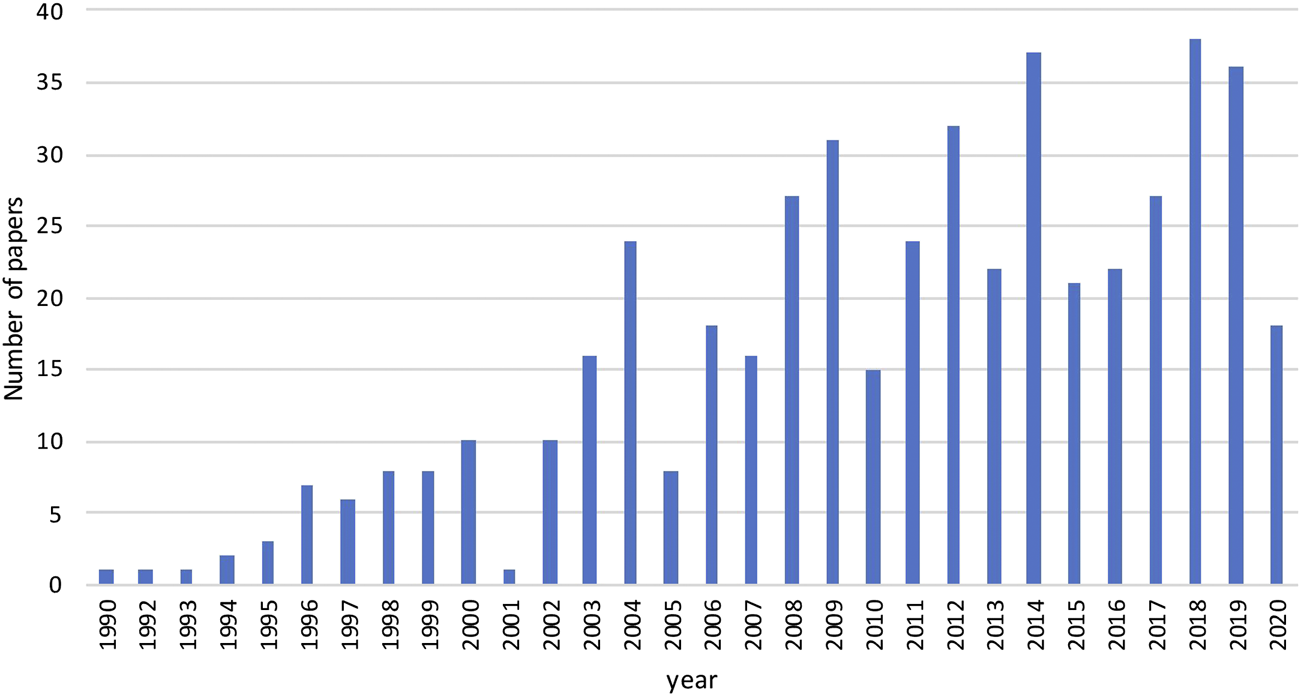
FIGURE 1. The number of papers published in journals including Computers and Chemical Engineering, Computer Aided Chemical Engineering, Industrial and Engineering Chemistry Research, and AIChE Journal from 1990 to September 1st, 2020 (Data obtained from Web of Science).

The applications of stochastic programming are also widespread in the PSE community. In Table 1, some highly cited papers from the four PSE-related journals that apply stochastic programming are reported. The applications have a very broad temporal scale, ranging from long-term design and planning problems to short-term scheduling and control problems. In terms of industrial sectors, the listed papers in Table 1 have both traditional industrial sectors, such as petroleum, natural gas, pharmaceutical, chemical, etc., and new sectors, such as biofuels, carbon capture, etc. The uncertainties that are considered in those applications include prices, supply, and concentration of raw materials, demands of final productions, process technologies, clinical trial outcomes.

TABLE 1

TABLE 1. Summary of representative works that use stochastic programming for PSE applications.

Given the increasing popularity of stochastic programming in the PSE community, this paper aims to give an overview of basic modeling techniques and algorithms for stochastic programming as well as a high-level description of the recent contributions made by the PSE community to a non-expert audience. For readers interested in the recent mathematical developments in stochastic programming, we refer to the review papers by Sahinidis (2004); Küçükyavuz and Sen (2017); Torres et al. (2019).

This paper is organized as follows. In Section 2, we provide an overview of mathematical programming and optimization under uncertainty. In Section 3, we introduce the concepts, mathematical formulations, and algorithms of two-stage stochastic programming. In Section 4, we introduce an extension of two-stage stochastic programming, multistage stochastic programming. In Section 5, the techniques for multistage stochastic programming under endogenous uncertainty are reviewed. In Section 6, we review data-driven methods for generating scenario trees. We draw the conclusion in Section 7.

2 Optimization Under Uncertainty

The decision-making process is normally modeled as an optimization problem. A generic optimization problem is represented in the following succinct form in Eq. 1 where we have some continuous variables x, to represent the decisions being made, (e.g. sizing decision of a reactor), 0–1 variables y to represent the discrete choices, (e.g. select a given reactor or not), an objective function f to minimize or maximize, (e.g. to minimize the total cost), and some constraints g, h, that the variables have to satisfy, (e.g. the mass balance).

$\underset{x,y}{\text{min}}f\left(x,y;\theta \right)$

$s.t.g\left(x,y;\theta \right)\le 0$

$h\left(x,y;\theta \right)=0$

$x\in {\mathbb{R}}^{n^x},y\in {\left\{\mathrm{0,1}\right\}}^{n^y}(1)$

Variables x are continuous variables with dimension n^x, which can take real values. Variables y are binary variables with dimension n^y, which can only take values 0 or 1. Binary variables are usually used to represent logic relations or choices e.g., whether to install a given chemical plant or not. Vector θ represents parameters involved in the optimization problem, such as product demand, unit costs of some processes. If we assume that these parameters are known with certainty, the problem Eq. 1 is a deterministic optimization problem. A deterministic optimization problem can be classified into several categories depending on the forms of f, g, h, x, y.

• some of f, g, h, are nonlinear functions. Problem Eq. 1 is a mixed-integer nonlinear program (MINLP).

• f, g, h are all linear functions. Problem Eq. 1 becomes a mixed-integer linear program (MILP).

• some of f, g, h, are nonlinear functions and there is no y variable, i.e., n^y = 0. Problem Eq. 1 becomes a nonlinear program (NLP).

• f, g, h, are linear functions and there is no y variable, i.e., n^y = 0. Problem Eq. 1 becomes a linear program (LP).

The four different mathematical programs, MINLP, MILP, NLP, LP, are chosen depending on the nature of the problem. For problems in chemical engineering, nonlinear equations are often used to describe thermodynamic or kinetic behavior. Integer variables can be used to describe process synthesis problems e.g., a binary variable can describe whether a given distillation column exists or not in a chemical flowsheet. For a detailed treatment of deterministic optimization methods, we refer to the textbook by Grossmann (2021).

In deterministic optimization models, parameters θ are assumed to be known. However, in practice, uncertainties are prevalent in process systems due to inaccurate measurement, forecast error, or lack of information. For example, uncertainties in supply chain management can arise from future customer demand, potential network disruption, or even the spread of a pandemic. Failing to consider uncertainties in the decision-making process may lead to suboptimal or even infeasible solutions. To hedge against the uncertainties in process systems, several mathematical frameworks have been used by the PSE community including stochastic programming, chance-constrained programming (Li et al., 2008), and robust optimization. (Lappas and Gounaris, 2016). The three approaches are different in their degrees of risk aversion and ways of characterizing uncertainties. Stochastic programming (SP) is a risk-neutral approach, which seeks to optimize the expected outcome over a known probability distribution. Chance-constrained programming can be seen as solving a stochastic program with some probabilistic constraints, which specify that some constraints with uncertain parameters are satisfied with a given level of probability. For example, a chance constraint can specify that a budget/cost that should not exceed a certain threshold. Chance constrained programming offers modeling flexibility to deal with reliability issues and have important connections with risk management. Robust optimization is another risk-averse approach, which seeks to optimize the “worst-case” over a pre-defined uncertainty set. Robust optimization problems typically involve min-max type of operators. A summary of the three approaches is shown in Table 2.

TABLE 2

TABLE 2. Summary of stochastic programming, chance-constrained programming, and robust optimization.

Besides these three approaches, there are a number of mathematical frameworks to model decision-making under uncertainty, such as Markov Decision Process (MDP). Powell (2019) unifies 15 communities in optimization under uncertainty in a single framework. Reviewing all the 15 approaches is outside the scope of this paper. Interested readers can refer to the relevant papers (Powell, 2019, Powell, 2016).

3 Two-Stage Stochastic Programming

Two-stage stochastic programming is a special case of stochastic programming. In this section, we describe the mathematical formulations, algorithms and illustrative examples for two-stage stochastic programming.

3.1 Two-Stage Stochastic Mixed Integer Linear Programs

For simplicity of presentation, we fist consider stochastic MILP problems.

3.1.1 Mathematical Formulation

In stochastic programming, it is assumed that the probability distributions of the uncertain parameters are known a priori. The uncertainties are usually characterized by some discrete realizations of the uncertain parameters as an approximation to the real probability distribution. For example, the realizations of the demand for a product can have three different values which represent high, medium, and low demand, respectively. Each realization is defined as a scenario. The objective of stochastic programming is to optimize the expected value of an objective function, (e.g. the expected cost) over all the scenarios.

A special case of stochastic programming is two-stage stochastic programming (Figure 2). Specifically, stage one decisions are made ‘here and now’ at the beginning of the period, and are then followed by the resolution of uncertainty. Stage two decisions, or recourse decisions, are taken ‘wait and see’ as corrective action at the end of the period. One common type of two-stage stochastic program is mixed-integer linear program presented in Eq. 2. Ω is the set of scenarios. τ_ω is the probability of scenario ω. x represent the first-stage decisions. y_ω represent the second-stage decisions in scenario ω. The uncertainties are reflected in the matrices (vectors), W_ω, h_ω, T_ω shown in Eq. 2. In the literature, W_ω is called the “recourse matrix”; T_ω is called the “technology matrix”. On the right of Figure 2, an example of a “scenario tree” that has three scenarios with uncertain h_ω is used to represent the realizations of uncertainties on the right hand side.

FIGURE 2

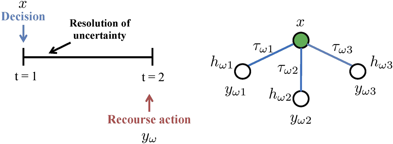
FIGURE 2. Two-stage problem: conceptual representation (left); scenario tree (right) where x represents the first stage decisions, $y_{\omega }$ represents the stage two decisions for scenario ω. ${\tau }_{\omega }$, $h_{\omega }$ represent the probability and the uncertain right hand side of scenario ω, respectively.

For problem Eq. 2, both the first and the second stage decisions are mixed-binary. Let $I=\left\{\mathrm{1,2},\dots ,n\right\}$ be the index set of all the first stage variables. $I_1\subseteq I$ is the subset for indices of the binary first stage variables. Let $J=\left\{\mathrm{1,2},\dots ,m\right\}$ be the index set of all the second stage variables. $J_1\subseteq J$ is the subset for the indices of the binary second stage variables. $x^{ub}$ is a vector that represents the upper bound of all the first stage variables. $y_{\omega }^{ub}$ is a vector that represents the upper bound of all the second stage variables. The problem described by Eq. 2 is a two-stage stochastic mixed-integer linear program (TS-MILP). If both J₁ and I₁ are empty sets, Eq. 2 reduces to a two-stage stochastic linear programming problem (TS-LP). Eq. 2 is often referred to as the deterministic equivalent or the extensive form of the two-stage stochastic program since Eq. 2 can be solved in the same way as if we were solving a deterministic optimization problem.

$\begin{array}{l}\min c^{\mathrm{\top }}x+{\displaystyle \sum _{\omega \in \Omega }{\tau }_{\omega }{d}_{\omega }^{\mathrm{\top }}{y}_{\omega }}\\ s.t.Ax\le b\\ W_{\omega }{y}_{\omega }\le h_{\omega }-T_{\omega }x\forall \omega \in \Omega \\ x\in X,X=\left\{x:x_i\in \left\{\mathrm{0,1}\right\},\forall i\in I_1,0\le x\le x^{ub}\right\}\\ y_{\omega }\in Y_{\omega }\forall \omega \in \Omega ,Y_{\omega }=\left\{y_{\omega }:y_{\omega j}\in \left\{\mathrm{0,1}\right\},\forall j\in J_1,0\le y_{\omega }\le y_{\omega }^{ub}\right\}.\end{array}(2)$

3.1.2 Process Network Problem

To show how two-stage stochastic programming can be applied to a process systems engineering problem, we provide a process network design problem under demand uncertainty. Through this example, we also aim to show that the solutions obtained from a stochastic program can be different from solving a deterministic problem where the uncertain parameters are fixed at their expected value.

Consider producing a chemical C which can be manufactured with either process 2 or process 3, both of which use chemical B as raw material. B can be purchased from another company and/or manufactured with process 1 which uses A as a raw material. The demand for chemical C, denoted as d, is the source of uncertainty. The superstructure of the process network is shown in Figure 3, which outlines all the possible alternatives to install this chemical plant. The alternatives include: 1) All three processes are selected. 2) A true subset of the three processes are selected. 3) None of the three processes are selected.

FIGURE 3

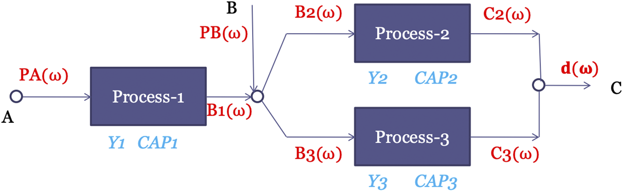
FIGURE 3. Superstructure for the process network problem.

Following the time realization framework described in Figure 2, the problem is formulated as a two-stage stochastic program. The chemical plant has to be first installed before the demand for the product is realized and the plant starts production. Therefore, the first-stage decisions are investment decisions on the three processes, which include binary variables Y_i to denote whether process i is selected and continuous variables CAP_i to denote the capacity of process i for i = 1, 2, 3. We assume that after the plant is installed, the demand for the product is realized. Based on the realizations of the demand, different recourse actions on how to operate the installed plant can be taken, i.e., the second-stage decisions are the material flows. We denote the scenarios as ω and explicitly state the dependency of the second-stage decision on them by presenting them as functions of ω.

Variables PA(ω), PB(ω) represent the purchase amount of chemical A and B, respectively. Other material flows for chemical B and C are shown in the superstructure in Figure 3. The MILP formulation is shown as follows.

$\begin{array}{l}\text{max}-\left(10Y_1+15Y_2+20Y_3+{\text{CAP}}_1+1.5{\text{CAP}}_2+2{\text{CAP}}_3\right)\\ +\underset{d\left(\omega \right)\sim \mathrm{\mathbb{P}}}{\mathbb{E}}\left[-4.5PA\left(\omega \right)-9.5PB\left(\omega \right)-0.5PA\left(\omega \right)-0.5B_2\left(\omega \right)-0.5B_3\left(\omega \right)+25C_2\left(\omega \right)+25C_3\left(\omega \right)\right]\end{array}(\mathrm{3a})$

$\text{s}.\text{t}.{\text{CAP}}_1\le U\cdot Y_1,{\text{CAP}}_2\le U\cdot Y_2,{\text{CAP}}_3\le U\cdot Y_3,Y_2+Y_3\le 1(\mathrm{3b})$

$PA\left(\omega \right)\le {\text{CAP}}_1,B_2\left(\omega \right)\le {\text{CAP}}_2,B_3\left(\omega \right)\le {\text{CAP}}_3\forall \omega (\mathrm{3c})$

$B_1\left(\omega \right)=0.9PA\left(\omega \right),C_2\left(\omega \right)=0.82B_2\left(\omega \right),C_3\left(\omega \right)=0.95B_3\left(\omega \right)\forall \omega (\mathrm{3d})$

$B_1\left(\omega \right)+PB\left(\omega \right)=B_2\left(\omega \right)+B_3\left(\omega \right)\forall \omega (3e)$

$C_2\left(\omega \right)+C_3\left(\omega \right)\le d\left(\omega \right)\forall \omega (\mathrm{3f})$

$Y_i\in \left\{\mathrm{0,1}\right\}\forall i\in \left\{\mathrm{1,2,3}\right\}(\mathrm{3g})$

The objective is maximizing the expected profit, which includes the expected income obtained from selling the final product $\left[25C_2\left(\omega \right)+25C_3\left(\omega \right)\right]$, minus the total cost that includes the fixed $\left(10Y_1+15Y_2+20Y_3\right)$ and variable $\left({\text{CAP}}_1+1.5{\text{CAP}}_2+2{\text{CAP}}_3\right)$ investment costs in stage one, the expected cost to purchase chemical A and B in different scenarios $\left[4.5PA\left(\omega \right)+9.5PB\left(\omega \right)\right]$) the expected operating cost $\left[0.5PA\left(\omega \right)+0.5B_2\left(\omega \right)+0.5B_3\right]$, which is proportional to the amount of input to each process, i.e., $PA\left(\omega \right)$, $B_2\left(\omega \right)$, $B_3\left(\omega \right)$.

Suppose we have a 3-scenario problem where the demands $d\left(\omega \right)$ take values $d\left({\omega }_1\right)=8$, $d\left({\omega }_2\right)=10$, $d\left({\omega }_3\right)=12$, with probabilities $\tau \left({\omega }_1\right)=0.25$, $\tau \left({\omega }_2\right)=0.5$, $\tau \left({\omega }_3\right)=0.25$, respectively. The optimal first-stage decisions are to select processes 1 and 3 with capacities 11.70 and 12.63, respectively, which is shown in Figure 4I. Note that the first-stage decisions are made “here-and-now” and thus are the same for all three scenarios. However, different second-stage decisions are taken for different scenarios as shown in Figure 4II. When the demand is low $d\left({\omega }_1\right)=8$, processes 1 and 3 are not operating at their full capacity. For $d\left({\omega }_2\right)=10$, process 1 is operating at full capacity but process 3 is not. For $d\left({\omega }_3\right)=12$, both installed processes are operating at full capacity. The chemical A produced by process 1 is not able to satisfy the requirement of process 3. Therefore, additional chemical B needs to be purchased from other vendors when the demand is high. The expected profit of the stochastic program is 117.22. This optimal value of the stochastic program is called the value of the recourse problem (RP) in the literature (Birge and Louveaux, 2011) (RP = 117.22).

FIGURE 4

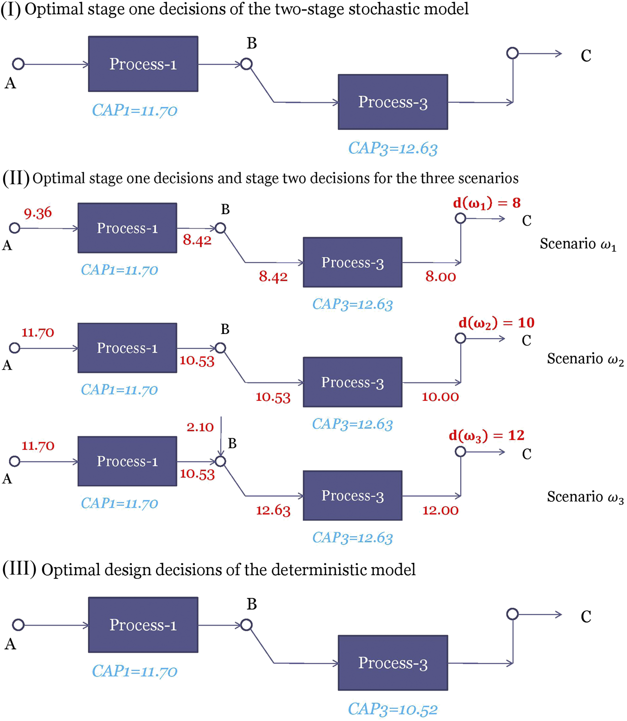
FIGURE 4. (I) represents the optimal first stage decisions of the two stage stochastic program (II) describes the optimal stage one decisions and the stage two decisions under scenarios ${\omega }_1$, ${\omega }_2$, ${\omega }_3$(III) represents the optimal design decisions of the deterministic model.

Other than using stochastic programming, an alternative approach is to solve the deterministic model where the demand is fixed at its mean value, i.e., set d = 10. The optimal solution for this deterministic model is selecting processes 1 and 3 with capacities being 11.70, and 10.52, respectively as shown in Figure 4III. The only difference from the stochastic solution is that the capacity of process 3 becomes lower. The reason is that the deterministic model is “unaware” of the high demand scenario and therefore makes the capacity of process 3 to be just enough to satisfy d = 10. However, if we use the deterministic solution for d = 12, it will result in lost sales. We can fix the first stage solutions to the optimal solutions and evaluate how it performs in the three scenarios by solving each stage two problem separately. An expected profit of 114.20 is obtained. This value is called the expected result of using the expected solution (EEV).

One quantitative metric to evaluate the additional value created by stochastic programming compared with solving the deterministic model at mean value is a concept called the value of the stochastic solution (VSS) (Birge and Louveaux, 2011). If the problem is a maximization problem, VSS is defined as,

$\text{VSS}=\text{RP}-\text{EEV}(4)$

Therefore, the value of the stochastic solution is 117.22 − 114.20 = 3.02 for the process network problem.

3.1.3 Classical Decomposition Algorithms

One option to solve the stochastic MILP problems described by Eq. 2 is to solve the deterministic equivalent problem Eq. 2 directly using commercial solvers like CPLEX, GUROBI. However, solving Eq. 2 directly can be prohibitive when the number of scenarios is large because the computational time can grow exponentially with the number of scenarios. Due to the difficulties in solving the deterministic equivalent problem, decomposition algorithms such as Lagrangean decomposition (Guignard, 2003; Oliveira et al., 2013) and Benders decomposition (Van Slyke and Wets, 1969; Laporte and Louveaux, 1993) can be applied to solve problem Eq. 2 more effectively.

A high-level view of the ideas behind Benders decomposition and Lagrangean decomposition is shown in Figure 5. The figure shows the structures of the constraint matrices where the columns correspond to the variables and the rows correspond to the constraints. Both decomposition algorithms take advantage of the “almost” block-diagonal structure shown in Figure 5.

FIGURE 5

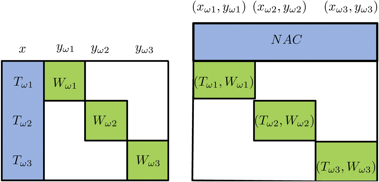
FIGURE 5. Schematic view of Benders decomposition (left; variables x are “complicating variables”), Lagrangean decomposition (right; the NACs are “complicating constraints”).

Benders decomposition (Van Slyke and Wets, 1969; Laporte and Louveaux, 1993), also referred to as L-shaped method in stochastic programming literature, views the first stage variables as “complicating variables” in the sense that if the first stage variables x are fixed the rest of problem Eq. 2 has a block-diagonal structure that can be decomposed by scenario and solved independently. A schematic view of the “complicating variable” idea behind Benders decomposition is shown in Figure 5. Mathematically, the Benders decomposition algorithm starts by defining a master problem with only the first-stage decisions. After the master problem is solved, the first-stage decisions are fixed at the optimal solution of the master problem. Then the deterministic equivalent problem can be decomposed into |Ω| subproblems where |Ω| denotes the cardinality of the set of scenarios. The subproblems can be solved in parallel and valid inequalities of x can be derived and added to the Benders master problem. The master problem is solved again and the algorithm iterates until the upper bound and the lower bound converge. The lower bound is the optimal value of the Benders master problem. The upper bound is obtained by updating the best feasible solution. Benders decomposition is able to converge in a finite number of steps when the second-stage decisions are all continuous and the second stage constraints are linear.

Lagrangean decomposition reformulates problem Eq. 2 by making a copy of the first-stage decisions for each scenario and adding non-anticipativity constraints (NACs) to ensure that the first-stage decisions made for all the scenarios are the same. For example, in a three-scenario problem, three copies of the x variables, $x_{{\omega }_1}$, $x_{{\omega }_2}$, $x_{{\omega }_3}$, are made. NACs including $x_{{\omega }_1}=x_{{\omega }_2}$, $x_{{\omega }_1}=x_{{\omega }_3}$ are added to guarantee the first-stage decisions are the same for all three scenarios. A schematic view of Lagrangean decomposition is also shown in Figure 5. After this reformulation, the NACs are then dualized so that the deterministic equivalent problem is decomposed into scenarios that can be solved in parallel. The Lagrangean multipliers can be updated using the subgradient method or the cutting plane method (Oliveira et al., 2013). A lower bound can be obtained at each iteration of Lagrangean decomposition which is the summation of the optimal value of the Lagrangean subproblems. However, the upper bound procedure of Lagrangean decomposition is in general a heuristic. Therefore, Lagrangean decomposition is not guaranteed to converge even for the problems with continuous recourse. There is usually a “duality gap” between the upper and the lower bound.

Although neither Benders nor Lagrangean decomposition are able to solve Eq. 2 with integer recourse variables to optimality with their classical form, recent developments have been made that can solve Eq. 2 to optimality by extending these two methods. A discussion of these recent advances can be too technical and we refer interested readers to the review papers, Torres et al. (2019); Küçükyavuz and Sen (2017), for details.

As for software implementations, the CPLEX solver has an implementation of the Benders decomposition algorithm Bonami et al. (2020), which can be accessed through most modeling platforms, such as GAMS, C, C++, Pyomo (Hart et al., 2017), Python, etc. DSP (Kim and Zavala, 2018) is a Lagrangean decomposition-based solver for two-stage stochastic mixed-integer programs, which provides interfaces that can read models expressed in C code and the SMPS format (Gassmann and Schweitzer, 2001). DSP can also read models expressed in JuMP (Lubin and Dunning, 2015).

3.2 Two-Stage Stochastic Mixed-Integer Nonlinear Programs

Most SP algorithms and applications investigated by the Operations Research (OR) community are (mixed-integer) linear problems as in Eq. 2. However, chemical engineering applications can involve significant nonlinearities. Examples include the mass balance equations for the splitters and mixers in a flowsheet, the MESH equations in distillation column design, the Arrhenius equation in reactor modeling. Therefore, developing stochastic programming models and algorithms for (mixed-integer) nonlinear problems is of great interest to chemical engineers doing PSE research. As a matter of fact, the PSE community has been the main driver of developing algorithms to efficiently solve stochastic MINLPs (Li et al., 2011b; Li and Grossmann, 2019b; Cao and Zavala, 2019).

3.2.1 Mathematical Formulation

The mathematical formulation of a general two-stage stochastic mixed-integer nonlinear program is shown in Eq. 5.

$\text{min}{f}_0\left(x\right)+{\displaystyle {\sum }_{\omega \in \text{Ω}}{\tau }_{\omega }{f}_1\left(x,y_{\omega };{\theta }_{\omega }\right)}$

$\text{s}\text{.t}\text{.}{g}_0\left(x\right)\le 0$

$g_1\left(x,y_{\omega };{\theta }_{\omega }\right)\le 0\forall \omega \in \text{Ω}$

$x\in X,X=\left\{x:x_i\in \left\{\mathrm{0,1}\right\},\forall i\in I_1,0\le x\le x^{ub}\right\}$

$y_{\omega }\in Y_{\omega },\forall \omega \in \text{Ω},Y_{\omega }=\left\{y_{\omega }:y_{\omega j}\in \left\{\mathrm{0,1}\right\},\forall j\in J_1,0\le y_{\omega }\le y_{\omega }^{ub}\right\}(5)$

Problem Eq. 5 is an extension of Eq. 2 by considering nonlinear objective and nonlinear constraints. Functions f₀, f₁, g₀, g₁ in Eq. 5 are nonlinear functions. f₁ and g₁ are functions of the first-stage decisions x, the second-stage decisions y_ω and the uncertain parameters θ_ω for scenario ω. Due to the nonlinear objective and the nonlinear constraints, Eq. 5 is more difficult to solve than Eq. 2. We will review the algorithms to solve Eq. 5 in Subsection 3.2.3.

3.2.2 Stochastic Pooling Problem Example

We provide an example of the stochastic pooling problem presented in Li and Grossmann (2019b). Pooling problem arises in applications include wastewater treatment (Karuppiah and Grossmann, 2008), crude oil refinery planning (Yang and Barton, 2016), and natural gas networks planning (Li et al., 2011a). Solving the pooling problem to optimality is of great interest due to potential savings in the order of tens of millions of dollars. In a pooling problem, flow streams from different sources are mixed in some intermediate tanks (pools) and blended again in the terminal points. At the pools and the terminals, the quality of a mixture is given as the weighted average of the qualities of the flow streams that go into them.

The pooling problem involves both design decisions and operating decisions. The design decisions are which feed i and which pool l to select from the superstructure shown in Figure 6A, and the sizing decisions for the selected feed tanks and pools. The second-stage decisions are the mass flowrates of different streams, and the split fractions. The operator has to operate the feeds and the pools to satisfy the quality specifications at the product terminals j (Figure 6A). In this problem, we also consider purchasing the feeds using three different types of contracts i.e., fixed price, discount after a certain amount, and bulk discount.

FIGURE 6

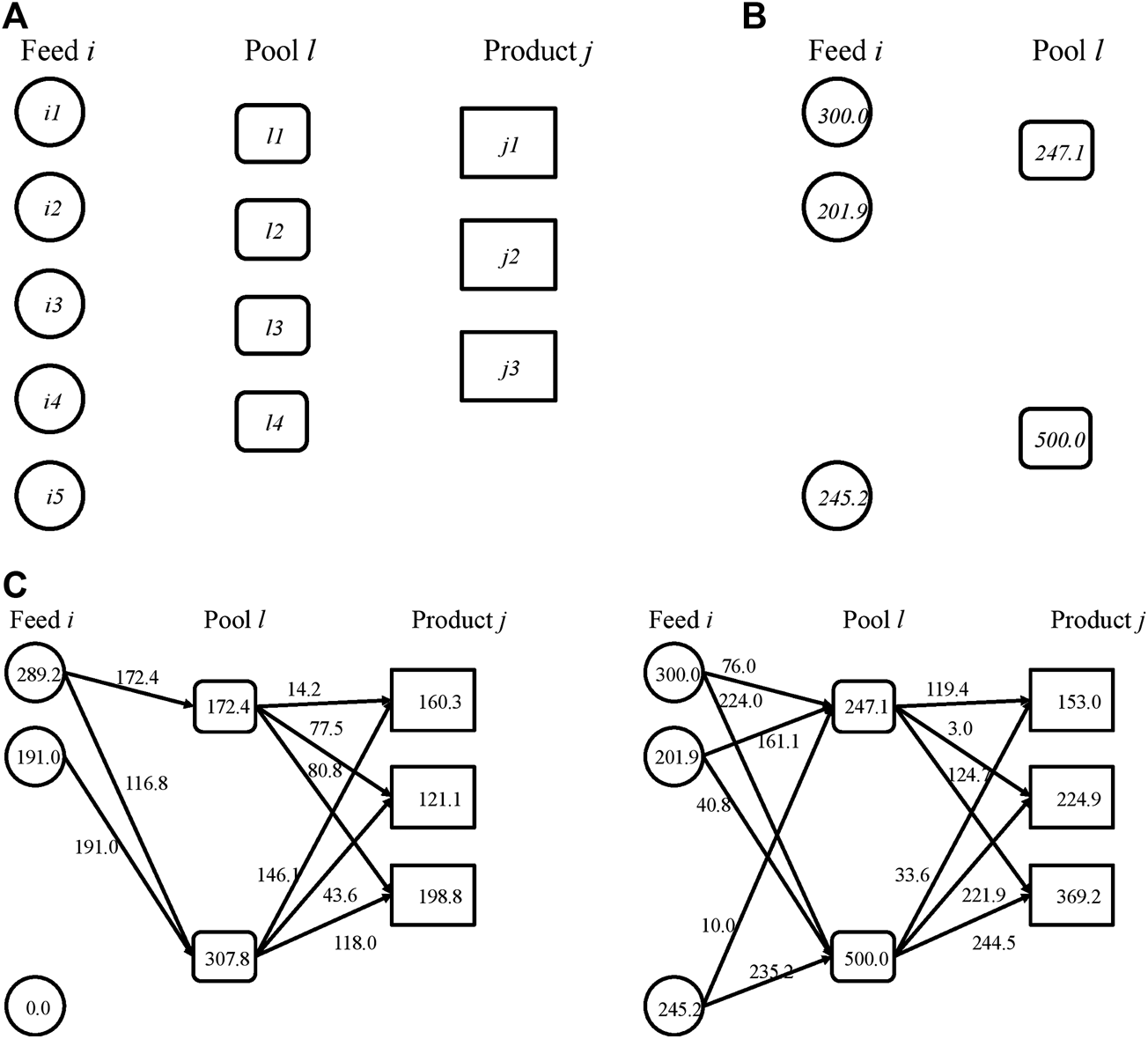
FIGURE 6. Stochastic pooling problem (A) is the superstructure of the pooling problem (B) is the optimal first-stage decisions for the pooling example (C) represents the optimal mass flow rates in the low-demand scenario (left) and the high-demand scenario (right).

Before the design decisions are made, several sources of uncertainties can arise at the operating level including quality of the feed streams, prices of the feeds and products, demands for the products. For this illustrative example, we only consider uncertainty in the demands of the products. The demands for the three products can take low, medium, and high values and are assumed to vary simultaneously i.e., there are three scenarios in this problem with probabilities 0.3, 0.4, 0.3, respectively. The actual delivered products have to be less than or equal to the demands. The objective is to maximize the expected total profit. The mathematical formulation of this problem has been reported in Li and Grossmann (2019b). To make this paper self-contained, we include the mathematical formulation in the supplementary material.

The deterministic equivalent of the stochastic pooling problem with three scenarios is solved to optimality. The optimal first-stage decisions are to select feeds i₁, i₂, i₅, pools l₁, and l₄. The optimal capacities of the selected feeds and pools are shown in Figure 6B. Recall that in two-stage stochastic programming, after the first-stage decisions are made, the uncertain demands are realized. In different scenarios, different recourse actions can be taken depending on the realization of the demand. The mass flow rates of all the streams in the high and the low demand scenarios can be seen in Figure 6C. When the demand is low, the feed tanks and the pools are not operating at their full capacities. When the demand is high, the feed tanks and pools are operating at their full capacities. Recall that the production of each product can be less than or equal to the demand. In the high-demand scenario, the production of product j₁ is even lower than that in the low-demand scenario. However, the productions of j₂ and j₃ are higher in the high-demand scenario than those in the low-demand scenario. The results also indicate that the optimal capacity is not enough to meet the high demand. The reason is that if one were to fully satisfy the high demand, a great part of the capacity would be left idle in the low-demand scenario. On the other hand, if the capacity were designed to be just enough to satisfy the low demand, there would be significant lost sales in the high-demand and the medium-demand scenarios. Stochastic programming is a “risk-neutral” approach to achieve the highest expected profit, which balances the trade-off between lost sales and idle capacity.

3.2.3 Algorithms for Solving Stochastic MINLP

As we discussed in Subsection 3.1.3, the classical decomposition algorithms, such as Benders decomposition and Lagrangean decomposition, cannot be readily applied to solve stochastic MINLPs. The challenges to solve stochastic MINLP problems are two-fold: the nonlinear functions in stage two can be nonconvex; second, some of the stage two variables need to satisfy integrality constraints, which also make the stage two problem nonconvex. Due to its wide application in process systems, researchers from the PSE community have been developing algorithms for solving problem Eq. 5. Most of the algorithms are based on the classical decomposition algorithms including Lagrangean decomposition, and generalized Benders decomposition (GBD) (Geoffrion, 1972) which is an extension of the Benders decomposition (BD) algorithm to convex nonlinear problems.

For convex stochastic MINLP, where the nonlinear feasible region of the continuous relaxation is convex, Li and Grossmann (2018) propose an improved L-shaped method where the Benders subproblems are convexified by rank-one lift-and-project, and Lagrangean cuts are added to tighten the Benders master problem. Li and Grossmann (2019a) further propose a generalized Benders decomposition-based branch and bound algorithm with finite ϵ-convergence for convex stochastic MINLPs with mixed-binary first and second stage variables.

For nonconvex stochastic MINLP, where the nonlinear functions in the stochastic MINLPs can be nonconvex, the pioneering work is done by Li et al. (2011b) who propose a nonconvex generalized Benders decomposition algorithm, which can solve two-stage nonconvex MINLPs with pure binary variables in a finite number of iterations. For the more general case where the first stage variables can be mixed-integer, Ogbe and Li (2019) propose a joint decomposition algorithm. A perfect information-based branch and bound algorithm that solves nonseparable nonconvex stochastic MINLPs to global optimality is proposed by Cao and Zavala (2019). Kannan (2018) propose a modified Lagrangean relaxation-based (MLR) branch and bound algorithm, and they prove that MLR has finite ϵ-convergence. A generalized Benders decomposition-based branch and cut algorithm for nonconvex stochastic MINLPs with mixed-binary first and second stage variables is proposed by Li and Grossmann (2019b). Li et al. (2020) propose a sample average approximation based outer approximation algorithm for stochastic MINLPs with continuous probability distributions.

4 Multistage Stochastic Programming

In two-stage stochastic programming, it is assumed that the uncertainties are realized only once after the first-stage decisions are made. However, most practical problems involve a sequence of decisions reacting to outcomes that evolve over time. A generalization of two-stage stochastic programming to the sequential realization of uncertainties is called “multistage stochastic programming”. The time horizon is discretized into “stages” where each stage has the realizations of uncertainties at the current stage.

A scenario tree similar to Figure 2 for a multistage problem is shown in Figure 7. The scenario tree has three stages. In stage two, there are two different realizations of uncertain parameters and therefore two nodes. Each of the two nodes can have different stage two decisions depending on the realization of information until stage two. After the stage two decisions are made, there are two different realizations of uncertain parameters at stage three for each node in stage two. Therefore, there are four nodes in total at stage three. The stage three decisions depend both on stage one, stage two decisions and the history of the uncertain parameters. A scenario in the multistage setting is a “path” from the root node of the scenario tree to the leaf node of the scenario tree, which corresponds to a full history of realization of uncertainty parameters until stage three. It is easy to see that there are 4 scenarios in Figure 7, represented using ω₁, ω₂, ω₃, ω₄. The seven nodes in the scenario tree are numbered sequentially with notation n₁−n₇.

FIGURE 7

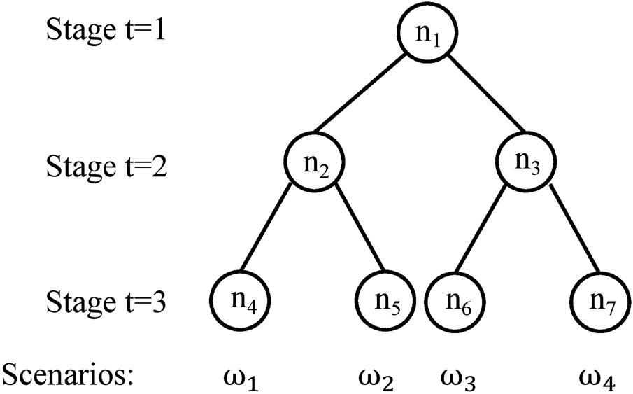
FIGURE 7. Illustration of a scenario tree with 3 stages, 4 scenarios, seven nodes.

It is worth pointing out that in some PSE applications, there are two types of decisions i.e., the strategic decisions e.g., the installation of chemical processes and the operational decisions e.g., material flow rates. The uncertainties can arise from both strategic and operational decision-making processes. A scenario tree that combines the two types of decisions and uncertainties can be found in Escudero and Monge (2018).

4.1 Mathematical Formulation

The general multistage stochastic programming formulation is given as follows (Birge and Louveaux, 2011):

$\text{min}{c}_1^{\mathrm{\top }}{x}_1+{\mathbb{E}}_{{\mathit{\xi }}_{[2,\mathit{H}]}|{\xi }_{\left[\mathrm{1,1}\right]}}\left\{\text{min}{c}_2^{\mathrm{\top }}\left({\xi }_2\right)x_2\left({\xi }_2\right)+\dots +{\mathbb{E}}_{{\mathit{\xi }}_{[\mathit{H}:\mathit{H}]}|{\xi }_{[1:H-1]}}\left[\text{min}{c}_H^{\mathrm{\top }}\left({\xi }_H\right)x_H\left({\xi }_H\right)\right]\right\}(\mathrm{6a})$

$\text{s}.\text{t}.W_1{x}_1\le h_1(\mathrm{6b})$

$T_2\left({\xi }_2\right)x_1+W_2{x}_2\left({\xi }_2\right)\le h_2\left({\xi }_2\right)(\mathrm{6c})$

$\dots (\mathrm{6d})$

$T_H\left({\xi }_H\right)x_{H-1}\left({\xi }_{H-1}\right)+W_H{x}_H\left({\xi }_H\right)\le h_H\left({\xi }_H\right)(6e)$

$x_1\in X_1;x_t\left({\xi }_t\right)\in X_t,t=2,\dots ,H;(\mathrm{6f})$

where we have H stages. For simplicity, we assume all the constraints and the objective function are linear. Suppose the data $\left({\mathit{\xi }}_2,\dots ,{\mathit{\xi }}_{\mathit{H}}\right)$ is uncertain and evolves according to a known stochastic process. We use ${\mathit{\xi }}_{\mathit{t}}$ to denote the random data vector in stage t and ${\xi }_t$ to denote a specific realization. The parameters $c_t$, $T_t$, $W_t$, $h_t$ are functions of ${\xi }_t$. Similarly, we use ${\xi }_{\left[t,t^{\prime }\right]}$ to denote the sequence of random data vectors corresponding to stages t through $t^{\prime }$ and ${\mathit{\xi }}_{\left[t,t^{\prime }\right]}$ to denote a specific realization of this sequence of random vectors. The decision dynamics is as follows: in stage t, we first observe the data realization ${\xi }_t$ and then take an action $x_t$ depending on the previous stage decision $x_{t-1}$ and the observed data ${\xi }_t$ to optimize the expected future cost. ${\mathbb{E}}_{{\mathit{\xi }}_{\left[\mathit{t},\mathit{H}\right]}|{\mathit{\xi }}_{\left[1,\mathit{t}-1\right]}}$ denotes the expectation operation in stage t with respect to the conditional distribution of ${\mathit{\xi }}_{\left[\mathit{t},\mathit{H}\right]}$ given realization ${\xi }_{\left[1,t-1\right]}$ in stage $t-1$. The constraints at stage t are defined for all the possible realizations of the stochastic process $\left({\mathit{\xi }}_2,\dots ,{\mathit{\xi }}_{\mathit{t}}\right)$ until stage t. Set $X_t$ denotes the domain of variables $x_t$, which can be continuous or (mixed)-integer. Eq. 6 can represent the deterministic equivalent of any multistage mixed-integer linear stochastic programs with discrete or continuous distributions.

For problems with discrete distributions, we can use the following node-based formulation,

$\underset{x_n}{\text{min}}\left\{{\displaystyle \sum }_{n\in \mathcal{N}}{\tau }_n{c}_n^{\mathrm{\top }}{x}_n:T_n{x}_{a\left(n\right)}+W_n{x}_n\le h_n,x_n\in X_n,\forall n\in \mathcal{N}\right\},(7)$

where set $\mathcal{N}$ denotes the set of nodes in the scenario tree. The decisions at node n is denoted as $x_n$. We use $a\left(n\right)$ to denote the ancestor nodes of node n. For example, in the scenario tree shown in Figure 7, the ancestor nodes of $n_4$ are $n_2$ and $n_1$, i.e., $a\left(n_4\right)=\left\{n_2,n_1\right\}$. ${\tau }_n$ is the probability of node n. The probability of a non-leaf node equals to the summation of the probabilities of its child nodes. For example, in Figure 7, ${\tau }_{n_2}={\tau }_{n_4}+{\tau }_{n_5}$. The decisions at a given node n, $x_n$, is dependent on the decision made at its ancestor nodes $x_{a\left(n\right)}$ and the realizations of the uncertain parameters until node n, which is reflected in $T_n$, $W_n$, and $h_n$.

An alternative way to write the deterministic equivalent of the node-based formulation is the following recursive formulations where set $\mathcal{C}\left(n\right)$ denotes all the child nodes of a node n. Parameter $q_{nm}$ denotes the transition probability from node n to its child node m. For example, in Figure 7, if nodes $n_4$, $n_5$ have equal probability, the transition probabilities from node $n_2$ to $n_4$ and $n_5$ are both 0.5.

$\underset{x\in X_1}{\text{min}}\left\{c_1^{\mathrm{\top }}{x}_1+{\displaystyle \sum }_{m\in \mathcal{C}\left(1\right)}{q}_{1m}{Q}_m\left(x_1\right):W_1{x}_1\le h_1\right\},(8)$

where for each node $n\in \mathcal{N}/\left\{1\right\}$, the cost-to-go function $Q_n$ is defined as

$Q_n\left(x_{a\left(n\right)}\right)=\left\{\underset{x_n\in X_n}{\text{min}}{c}_n^{\mathrm{\top }}{x}_n+{\displaystyle \sum }_{m\in \mathcal{C}\left(n\right)}{q}_{nm}{Q}_m\left(x_n\right):W_n{x}_n\le h_n-T_n{x}_{a\left(n\right)}\right\}.(9)$

For the terminal condition $t=H$, the set $\mathcal{C}\left(n\right)$ is be empty.

4.2 Multistage Process Network Problem

To provide an illustrative example for multistage stochastic programming, the two-stage process network design problem in Subsection 3.1.2 is extended to a three-stage problem. Stage one decisions are the same as those in Section 3.1.2 i.e., the selection of the three processes and the capacities of the selected processes. After the design decisions at stage one are made, the demand in stage two are realized. Besides the operating decisions on the installed plant, the decisions at stage two include capacity expansion decisions on the installed processes. We assume that the expanded capacity will be available at stage three. After the stage two decisions are made, the demand at stage three is realized. The stage three decisions only include the operating decisions i.e., the material flow rates. The objective is to maximize the expected total profit over all the scenarios.

The scenario tree is assumed to have two realizations per stage, which has the same structure as the scenario tree in Figure 7. We use $d_n$ to denote the realization of demand at node n. The demand at stage two is assumed be take two different values, $d_{n_2}=8$, $d_{n_3}=12$. The two child nodes, $n_4$ and $n_5$, of node $n_2$, are assumed to take values $d_{n_5}=8$, $d_{n_6}=10$, whereas, the two child nodes, $n_6$ and $n_7$, of node $n_3$, are assumed to take higher values i.e., $d_{n_6}=12$, $d_{n_7}=14$. The four scenarios are assumed to have equal probabilities.

The optimal solution of multistage stochastic process network design problem corresponding to nodes $n_2,\dots ,n_7$ are shown in Figure 8. The material flowrates at each node are shown in red. The installed capacities at the previous stage are shown in blue italics. At stage one, process one and three are selected and can be used in stage two. At stage two, when the demand is low i.e., $d_{n_2}=8$, processes 1 and 3 are not operating at full capacity. When the demand is high i.e., $d_{n_3}=12$, both process one and process three are operating at full capacity. Process three is expanded at stage two when the high demand is observed. The expanded capacity can be used in stage three at nodes $n_6$ and $n_7$. The stage three decisions are the material flow rates of different chemicals. At node $n_4$, $n_5$, and $n_6$, the installed process one and three are able to satisfy the demand. At node $n_7$, due to the limited capacity of process 1, additional chemical B needs to be purchased.

FIGURE 8

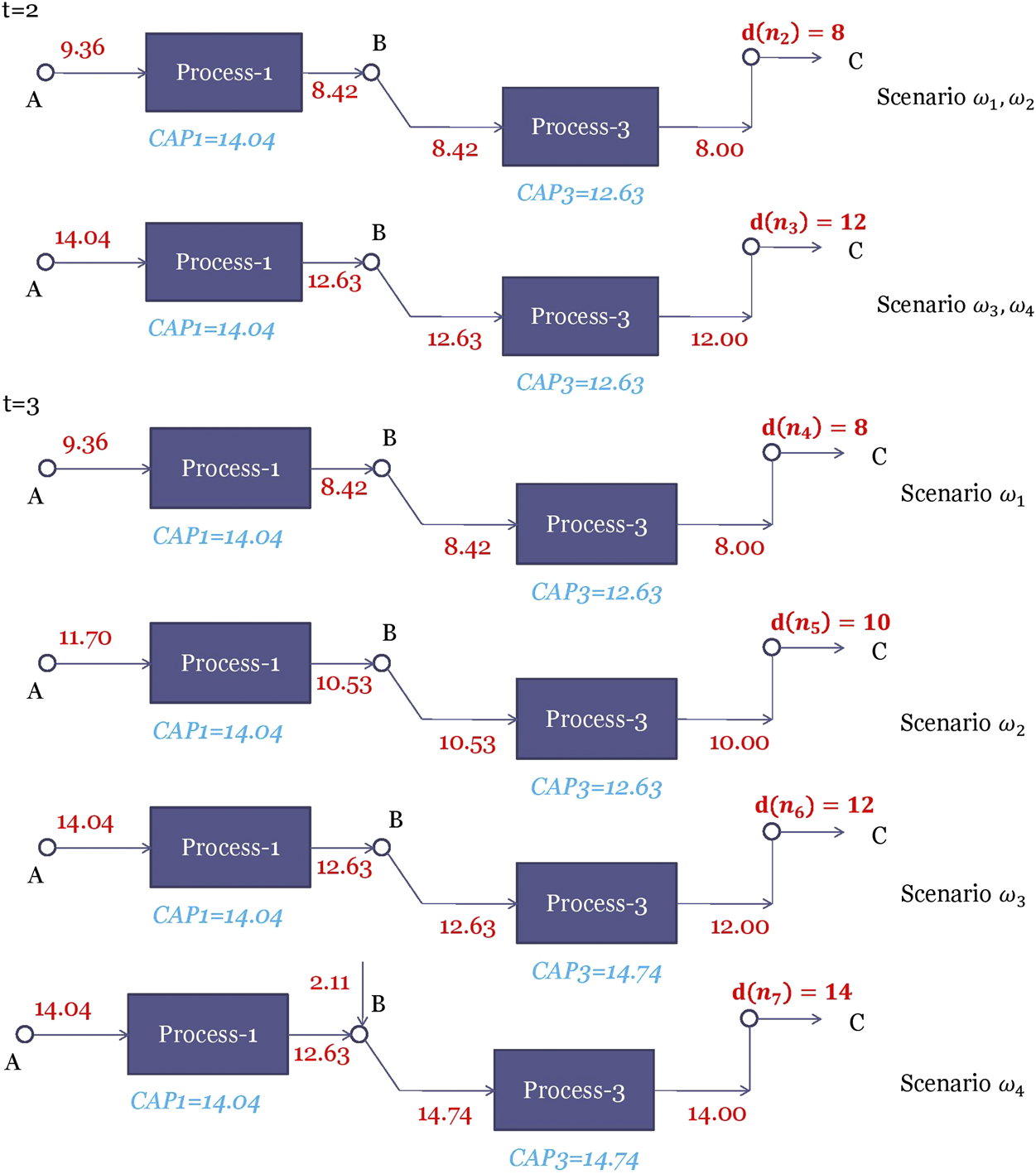
FIGURE 8. Optimal solutions of the stochastic process network design problem corresponding to nodes $n_2,\dots ,n_7$. The material flow rates at each node are shown in red. The installed capacities are shown in blue italics.

4.3 Algorithms for Multistage Stochastic (Mixed-Integer) Linear Programs

The number of scenarios of a multistage stochastic program grows exponentially with the number of stages. For example, suppose we have three different realizations of uncertain parameters at each stage, the number of scenarios for a problem with H stages is $3^{H-1}$. Therefore, special decomposition algorithms are usually applied to solve multistage stochastic programming problems. Most of the algorithms for multistage stochastic programs are based on classical Benders and Lagrangean decomposition algorithms.

An extension of Benders decomposition to multistage stochastic linear programs is called “nested Benders decomposition” (Birge, 1985). The idea is to apply Benders decomposition recursively to the multistage problem. Nested Benders decomposition has a “forward pass” step and a “backward pass” step. In the forward pass step, feasible solutions are generated by sequentially solving the root node of the scenario tree all the way to the leaf nodes of the scenario tree. Problem Eq. 9 for node n is solved “locally” in the forward pass with the value of $x_{a\left(n\right)}$ fixed from the solution of its parent node and the expected cost to go function $Q_m\left(x_n\right)$ approximated by some cutting planes generated from the backward pass. In the backward pass, the problems are solved sequentially from the leaf nodes to the root node. Cutting planes are generated in the backward pass to refine the approximations for the cost-to-go functions $Q_m\left(x_n\right)$.

Although the nested Benders decomposition algorithm can decompose the fullspace problem by nodes, it still has to solve an exponential number of leaf nodes. An algorithm that avoids solving an exponential number of nodes is the stochastic dual dynamical programming (SDDP) algorithm (Pereira and Pinto, 1991). One caveat to apply SDDP is that the underlying stochastic process has to be stagewise-independent i.e., the realizations of ${\mathit{\xi }}_{\mathit{t}}$ do not dependent on the history ${\xi }_{\left[1,t-1\right]}$. The idea of SDDP is that the cutting plane can be shared among the nodes under the stagewise-independence assumption and thus avoiding solving an exponential number of nodes. An extension of SDDP that can solve multistage stochastic mixed-integer linear program is the stochastic dynamic dual integer programming (SDDiP) algorithm proposed by Zou et al. (2019). Besides the standard Benders cuts, the authors propose to use other families of cutting planes including Lagrangean cuts, integer cuts, and strengthened Benders cuts. Applications of SDDiP have been reported in Escudero et al. (2020); Zou et al. (2018); Lara et al. (2019).

Lagrangean decomposition can be adapted to solve multistage stochastic programs in a similar way to two-stage by duplicating the variables such that each scenario has its own copy of variables at each stage and adding nonanticipativity constraints (NACs). The scenario tree in Figure 7 can be expressed in an alternative form shown in Figure 9 (Ruszczyński, 1997). The node in the first stage in Figure 7 is duplicated for each scenario ω and NACs (shown in red in Figure 9) are added to guarantee that the first stages decisions are the same for all the scenarios. Each node in stage two in Figure 7 is duplicated once and NACs are added to guarantee that the scenarios with the same parent node in Figure 7 have the same second-stage decisions. With the alternative scenario tree, Lagrangean decomposition dualizes the NACs and solves each scenario independently.

FIGURE 9

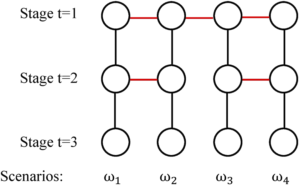
FIGURE 9. An alternative form of the scenario tree with 3 stages, 4 scenarios.

One major difference between nested Benders decomposition and Lagrangean decomposition is that nested Benders decomposition decomposes the fullspace problem by nodes, whereas Lagrangean decomposition decompose the fullspace problem by scenarios. A discussion of the trade-offs are not within the scope of this paper and can be found in Torres et al. (2019). Moreover, a recent review on main types of decomposition algorithms for two-stage and multistage stochastic mixed integer linear optimization can be found in Escudero et al. (2017).

As for software packages for multi-stage stochastic programs, SDDP. jl (Dowson and Kapelevich, 2020) is an implementation of the SDDP algorithm in Julia that is built on the JuMP modeling tools (Lubin and Dunning, 2015). MSPPy (Ding et al., 2019) is an implementation of the SDDP/SDDiP algorithm in Python. PySP (Watson et al., 2012) is an implementation of the progressive hedging algorithm (Rockafellar and Wets, 1991), an algorithm that can be seen as an augmented Lagrangean decomposition, in Pyomo (Hart et al., 2017).

5 Multistage Stochastic Programming Under Endogenous Uncertainty

In the stochastic programming models that we have discussed in the last few sections, the underlying stochastic processes are independent of the decisions. This type of uncertainty is called “exogenous” uncertainty. Another type of uncertainty that is decision-dependent is called “endogenous” uncertainties. There two distinct types of endogenous uncertainties commonly denoted as Type 1 and Type 2 in the literature (Goel and Grossmann, 2006).

In the case of Type 1 endogenous uncertainties, decisions influence the parameter realizations by altering the underlying probability distributions for the uncertain parameters. A simple example of this may be an oil company’s decision to flood the market in order to force a competitor out of business. Here the uncertainty is no longer strictly exogenous, as the decision will make lower oil-price realizations more likely. Type 1 endogenous has not been widely studied.

In the case of Type 2 endogenous uncertainties, decisions influence the parameter realizations by affecting the time at which we observe these realizations. This refers specifically to technical parameters, such as oilfield size, for which the true values cannot be determined until a particular investment decision is made. The modeling framework and algorithm for stochastic programming with Type 2 endogenous uncertainty are first proposed by Goel and Grossmann (2006). Since then, this approach has been adopted by the PSE community to address problems in a wide range of applications including oil and gas field planning (Goel and Grossmann, 2004), synthesis of process networks (Tarhan and Grossmann, 2008), pharmaceutical industry (Colvin and Maravelias, 2008; Christian and Cremaschi, 2015), etc.

Here, we describe the modeling framework proposed by Goel and Grossmann (2006). Figure 10 shows a scenario tree for a three-stage problem with two endogenous uncertain parameters, ${\theta }_1$, ${\theta }_2$. Both parameters are assumed to have two realizations i.e., ${\theta }_1\in \left\{{\widehat{\theta }}_1^L,{\widehat{\theta }}_1^H\right\}$, ${\theta }_2\in \left\{{\widehat{\theta }}_2^L,{\widehat{\theta }}_2^H\right\}$. We consider the combinations of the two realizations for ${\theta }_1$ and ${\theta }_2$. There are four scenarios in total with realizations, $\left\{{\widehat{\theta }}_1^L,{\widehat{\theta }}_2^L\right\}$, $\left\{{\widehat{\theta }}_1^L,{\widehat{\theta }}_2^L\right\}$, $\left\{{\widehat{\theta }}_1^L,{\widehat{\theta }}_2^L\right\}$, $\left\{{\widehat{\theta }}_1^L,{\widehat{\theta }}_2^L\right\}$, respectively. The scenario tree in Figure 10 is a scenario-based representation i.e., the decisions are duplicated for each scenario and NACs are added. However, the way that the NACs are added in Figure 10 is different than that in Figure 9 because the realizations of the uncertain parameters are decision-dependent. In stage one, since the decisions have not been made to reveal the values of the uncertain parameters, “initial NACs” are added to guarantee that the first-stage decisions are the same for all the scenarios. The initial NACs are represented using solid red lines in Figure 10. For stage two and three, the NACs are added conditionally, depending on whether the corresponding decisions are made in order to reveal the uncertain parameters. These NACs are called “conditional NACs”, which are shown in Figure 10 as dashed blue lines.

FIGURE 10

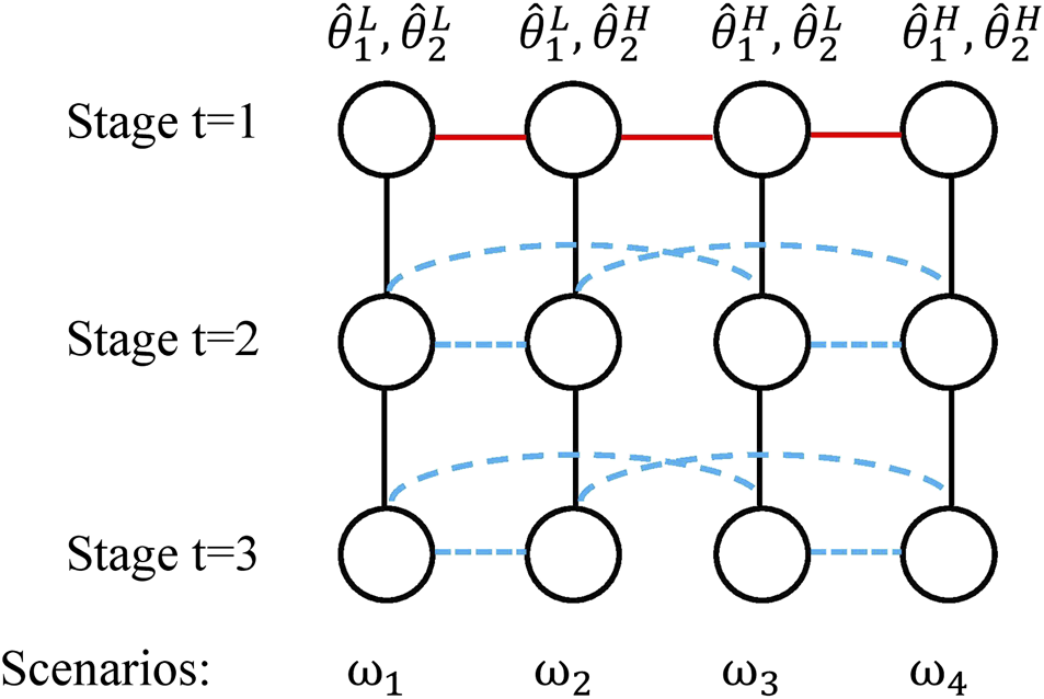
FIGURE 10. Illustration of the scenario tree of a stochastic programming problem under endogenous uncertainty with 3 stages, four scenarios, two uncertain parameters ${\theta }_1$, ${\theta }_2$.

To provide a concrete example, suppose ${\theta }_1$ and ${\theta }_2$ are the sizes of two undeveloped oil fields, $o_1$ and $o_2$, respectively, the decisions to reveal the sizes are the drilling of oil field 1 and 2. We use binary variable $b_{ot}$ to denote whether oil field o is drilled at stage t. At $t=1$, since no oil fields have been drilled before $t=1$ and no information regarding the size of the oil fields has been obtained, the decisions for all the four scenarios are the same i.e., we need to add the initial NACs. At $t=1$, if the operator decides to drill $o_1$, then the realization of ${\theta }_1$ will be known before stage 2. At stage two, the scenarios with ${\theta }_1={\widehat{\theta }}_1^L$ and the scenarios with ${\theta }_1={\widehat{\theta }}_1^H$ can be distinguished. Conditional NACs will only be added for the scenario pairs $\left({\omega }_1,{\omega }_2\right)$, and $\left({\omega }_3,{\omega }_4\right)$. On the other hand, if the operator decides not to drill any oil fields at $t=1$, the four scenarios are still indistinguishable at the beginning of stage two, all the conditional NACs at stage two have to be enforced.

5.1 Mathematical Formulation

The mathematical formulation for the multistage stochastic programming problem under endogenous uncertainty is,

$\text{min}{\displaystyle \sum }_{\omega \in \text{Ω}}{\tau }_{\omega }{\displaystyle \sum }_{t\in \mathcal{T}}{c}_{t,\omega }^{\mathrm{\top }}{x}_{t,\omega }(\mathrm{10a})$

$\text{s}.\text{t}.{\displaystyle \sum }_{t\text{'}=1}^t{A}_{t^{\prime },t,\omega }{x}_{t^{\prime },\omega }\le b_{t,\omega }\forall t\in \mathcal{T},\omega \in \text{Ω}(\mathrm{10b})$

$x_{1,\omega }=x_{1,{\omega }^{\prime }},\forall \left(\omega ,{\omega }^{\prime }\right)\in \mathcal{S}{\mathcal{P}}_{\mathcal{F}}(\mathrm{10c})$

$\left[\begin{array}{c}{Y}_{t,\omega ,{\omega }^{\prime }}\\ x_{t+1,\omega }=x_{t+1,{\omega }^{\prime }}\end{array}\right]\vee \left[\begin{array}{c}{Y}_{t,\omega ,{\omega }^{\prime }}\end{array}\right]\forall \left(\omega ,{\omega }^{\prime }\right)\in \mathcal{S}{\mathcal{P}}_{\mathcal{N}},t\in \mathcal{T}(\mathrm{10d})$

$Y_{t,\omega ,{\omega }^{\prime }}\iff F\left(x_{1,\omega },\dots ,x_{t,\omega }\right)\forall \left(\omega ,{\omega }^{\prime }\right)\in \mathcal{S}{\mathcal{P}}_{\mathcal{N}},t\in \mathcal{T}(10e)$

$x_{t,\omega }\in X_t,\forall t\in \mathcal{T},\omega \in \text{Ω}(\mathrm{10f})$

$Y_{t,\omega ,{\omega }^{\prime }}\in \left\{\text{True},\text{False}\right\}\forall \left(\omega ,{\omega }^{\prime }\right)\in \mathcal{S}{\mathcal{P}}_{\mathcal{N}},t\in \mathcal{T}(\mathrm{10g})$

where $x_{t,\omega }$ denotes the decisions made at stage t in scenario ω. $Y_{t,\omega ,{\omega }^{\prime }}$ is a Boolean variable that equals to True if the two scenarios ω and ${\omega }^{\prime }$ are indistinguishable at stage t. The objective function Eq. 10a is to minimize the expected cost. Eq. 10b represents constraints that govern decisions $x_{t,\omega }$ and link decisions across time periods. The initial NACs are expressed in Eq. 10c, where set $\mathcal{S}{\mathcal{P}}_{\mathcal{F}}$ represents the set of scenario pairs to enforce the initial NACs. The scenario pairs for the initial NACs can be written similar to the NACs in the exogenous case. Eq. 10d represents the conditional NACs where set $\mathcal{S}{\mathcal{P}}_{\mathcal{N}}$ represents the scenario pairs that differ in the realization of only one endogenous parameter (Goel and Grossmann, 2004). If the two scenarios ω and ${\omega }^{\prime }$ are indistinguishable at stage t i.e., $Y_{t,\omega ,{\omega }^{\prime }}=\text{True}$, NACs are added for the decisions in the next time period. Otherwise, no NACs are added. The value of the Boolean variable is determined by the decisions made at and prior to time t, which is expressed in a general form in Eq. 10e. In the oil field example, the expression $F\left(x_{1,\omega },\dots ,x_{t,\omega }\right)$ is to determine whether a given oil field has been developed based on the drilling decisions. Eqs. 10f and 10g specify the domain of variables $x_{t,\omega }$ and $Y_{t,\omega ,{\omega }^{\prime }}$.

We acknowledge that the mathematical formulation in Eq. 10 is a succinct form for ease of explanation. For a more detailed and rigorous formulation, we refer the readers to the paper by Apap and Grossmann (2017). See also Hellemo et al. (2018) for a nonlinear modeling approach.

5.2 Multistage Process Network Design Under Endogenous Uncertainty

To provide an illustrative example for multistage stochastic programming under endogenous uncertainty, the two-stage process network design problem in Subsection 3.1.2 is modified to a three-stage problem where the uncertainty is assumed to come from the yield of process one and the demand is assumed to be deterministic. In practice, process one can be a new technology that has never been installed before. Once process one is installed, its yield will be realized in the next stage. Therefore, the time of realization is decision-dependent. We assume that there are two realizations of the yield of process one i.e., two scenarios, being 0.9, and 0.8 with equal probability, which is denoted as $\text{Yield}\left({\omega }_1\right)=0.9$, $\text{Yield}\left({\omega }_2\right)=0.8$, $\tau \left({\omega }_1\right)=0.5$, $\tau \left({\omega }_2\right)=0.5$

For this problem, stage one decisions are the same as those in Subsection 3.1.2 i.e., the selection of the three processes and the capacities of the selected processes. At stage two, besides the operating decisions on the installed plant, the capacity of the processes that have been installed at stage one can be expanded; the processes that have not been installed at stage one can also be selected and installed at stage two. The installed and expanded processes will be available at stage three. The stage three decisions only include the operating decisions i.e., the material flow rates. The objective is to maximize the expected total profit over all the scenarios.

Three cases can happen for the realization of the yield uncertainty:

(1) Process 1 is selected at stage one. The uncertainty of the yield is realized at stage two. Only the initial NACs are active.

(2) Process 1 is selected at stage two. The uncertainty of the yield is realized at stage three. The initial NACs and the NACs for stage two decisions are active.

(3) Process 1 is never selected. The uncertainty of the yield is never realized. The initial NACs and the NACs for stage two and stage three decisions are active.

The optimal solution is shown in Figure 11. Processes 1 and 3 are selected at stage one. The yield of process 1 is realized at stage two. The capacity of process 1 installed at stage one is chosen such that it is only able to produce enough chemical B if the yield is high. On the other hand, if the yield of process 1 is low, additional chemical B needs to be purchased at stage two. Since the two scenarios can be distinguished at stage two, additional capacity for process 1 is added in the high-yield scenario such that enough chemical B can be produced by process 1 when the demand is increased to 14 at stage three. For the low-yield scenario, it is not profitable to produce chemical B from process 1. Therefore, no capacity for process 1 is added in stage two. The inadequacy of chemical B is resolved by purchasing from other suppliers.

FIGURE 11

FIGURE 11. Optimal solution of the three-stage process network problem under endogenous uncertainty.

In order to see the value of the stochastic solution, we solve a deterministic problem with the yield fixed at mean value i.e., 0.85. The optimal solution of the deterministic model is to select processes 1 and 3 as well. However, the capacity of process 1 at stage one is 12.38 instead of 11.70 as in the stochastic model. This capacity is chosen such that enough chemical B can be produced at stage two when the yield is 0.85. This capacity is suboptimal if the actual yield can be 0.8 or 0.9.

5.3 Algorithms for Solving Stochastic Programming Under Endogenous Uncertainty

Solving stochastic programs under endogenous uncertainties can be even more challenging than solving the stochastic programs under exogenous uncertainties because of the additional binary variables involved in reformulating the disjunctions in the conditional NACs Eq. 10d. To reduce the number of redundant NACs, scenario pair reduction techniques have been proposed Goel and Grossmann (2006); Boland et al. (2016); Apap and Grossmann (2017). However, even with a reduced number of scenario pairs, the deterministic equivalent (10) of problems with a large number of scenarios is still intractable. Goel and Grossmann (2006) propose a Lagrangean decomposition-based branch and bound algorithm that dualizes the initial NACs and relax the conditional NACs. To satisfy the NACs, the authors propose to branch on the logical variables $Y_{t,\omega ,{\omega }^{\text{'}}}$, and the variables involved in the constraints that are dualized. The Lagrangean decomposition-based algorithm is able to provide both feasible solutions and a lower bound for the stochastic programs. Colvin and Maravelias (2008) propose a branch and cut algorithm where necessary non-anticipativity constraints that are unlikely to be active are removed from the initial formulation and only added if they are violated within the search tree.

Others have proposed heuristic algorithms that can quickly obtain feasible solutions to (10). Christian and Cremaschi (2015) apply a knapsack decomposition algorithm (KDA) to the pharmaceutical R&D pipeline management problem. Zeng et al. (2018) extend the KDA algorithm to a generalized knapsack-problem based decomposition algorithm (GKDA). Apap and Grossmann (2017) propose a sequential decomposition algorithm for stochastic programs under both exogenous and endogenous uncertainties.

6 Data Driven Scenario Tree Generation

The crucial assumption in stochastic programming is that a scenario tree is given to characterize the probability distribution of the underlying stochastic process. The values and probabilities in the scenario tree affect the optimal solutions obtained from the stochastic programs. A poor scenario-generation method can spoil the result of the whole optimization model. In this section, we review the concepts and algorithms of scenario tree generation. Note that the notations used here are for exogenous uncertainty. The concepts and methods can be easily extended to problems with endogenous uncertainty.

The sources of data for generating scenarios can come from historical data, time-series model, or expert knowledge (Kaut, 2011). Historical data represents reliable past information but can generalize poorly in the future. Statistical or time-series models such as autoregressive integrated moving average (ARIMA), hidden Markov model (HMM), might generalize well in the future but usually need to be fit by data. Expert knowledge is useful in certain applications. For example, the prediction of oil price needs expertise in geopolitics. In practice, usually, a combination of all the three approaches is used i.e., estimate the distribution from historical data, then use a mathematical model and/or expert knowledge to adjust the distribution to the current situation.

A good scenario tree should capture the distributions of the random variables at each time period and the inter-temporal dependencies. The distributions at each time period can be characterized by the marginal distributions of all the variables, or more succinctly by their means and higher-order moments. Furthermore, the dependence of the variables is usually measured by their correlations. The inter-temporal dependencies describe how the realizations in the previous time periods affect the distributions at the current period. These dependencies are typically modeled by time-series models.

The time series models are inherently continuous probability distributions of the random variables. A scenario tree can be seen as a discrete approximation of a time-series model. The quality of a scenario tree generation method can be evaluated by the stability and the error of this approximation. The stability measures the deviation of the optimal solutions if the generation method is applied multiple times to generate the scenario trees. The error measures the suboptimality in the objective value resulted from the discrete approximation. The quantitative descriptions of the stability and error in scenario tree generation can be found in Kaut and Wallace (2003).

6.1 Sampling-Based Scenario Generation Methods

A common way to generate scenario trees is to generate i. i.d. (independent and identically distributed) samples from the “true” distribution through a simulation. For example, in the case of two-stage stochastic programming, we represent “true” stochastic programming problem succinctly as,

$z^{\text{*}}=\underset{x}{\text{min}}\underset{\theta \sim \mathrm{\mathbb{P}}}{\mathbb{E}}f\left(x;\theta \right),(11)$

where x is the first stage variables, $\mathrm{\mathbb{P}}$ denotes the “true” distribution, θ denotes the random variables. The stage two problem is contained implicitly in function f. Solving Eq. 11 with a continuous distribution directly is usually computationally intractable due to the integration over the continuous distribution. Suppose we can generate N i. i.d. samples, ${\theta }_1,\dots ,{\theta }_N$ from $\mathrm{\mathbb{P}}$, (11) can be approximated by the following sample average approximation (SAA) problem (Shapiro et al., 2014),

$z^N=\underset{x}{\text{min}}\frac{1}{N}{\displaystyle \sum }_{i=1}^{N}f\left(x;{\theta }_i\right)(12)$

where the true distribution $\mathrm{\mathbb{P}}$ is approximated by the empirical distribution of the N i. i.d. samples. It can be proved that as $N\to \infty$, the optimal value and solutions of Eq. 12 converge to the optimal value and solutions of Eq. 11 under some mild assumptions (Shapiro et al., 2014). However, generating an infinite number of samples is impractical. Sample size estimates for finite error have been developed (Kleywegt et al., 2002; Shapiro et al., 2014) for different types of two-stage stochastic programs. These estimates are usually too conservative for real-world problems. A practical implementation of the sample average approximation is proposed by Kleywegt et al. (2002).

There are several advantages to the SAA method. It is easy to implement if it is possible to sample from the true distribution. It also has very good asymptotic and finite convergence properties. However, SAA can have poor performance and stability if a small number of samples are used, especially for probability distributions with large variances. More importantly, we have to know the “true” distribution to sample from.

6.2 Property Matching Methods

The idea behind the property matching methods is to construct the scenario trees in such a way that some given properties of the “true distribution” are matched. The properties are, for example, the moments of the marginal distributions and covariances/correlations. Høyland and Wallace (2001) propose a nonlinear programming approach to matching the moments of the scenario tree to those estimated from a dataset or a continuous distribution. The unknowns in the nonlinear programming problem are the probabilities and values of the scenarios with the number of scenarios fixed.

However, with the moments alone, the matching problem is usually under-specified, especially if the number of realizations in the scenario tree is large i.e., the scenario tree is able to match the moments perfectly and there are still some degrees of freedom left. To address the under-specification issue, Calfa et al. (2014) propose to match both the moments and the cumulative distribution function (CDF) of the empirical distribution that are derived from real-world data. For example, in Figure 12, the blue dots represent the empirical CDF constructed from some production yield data. Since the empirical distribution is discontinuous and difficult to match in an optimization problem, Calfa et al. (2014) propose to fit a Generalized Logistic Function (GLF) with the data points of the empirical distribution.

$\text{GLF}\left(x\right)={\beta }_0+\frac{{\beta }_1-{\beta }_0}{{\left(1+{\beta }_2{e}^{-{\beta }_{3}x}\right)}^{1/{\beta }_4}}(13)$

FIGURE 12

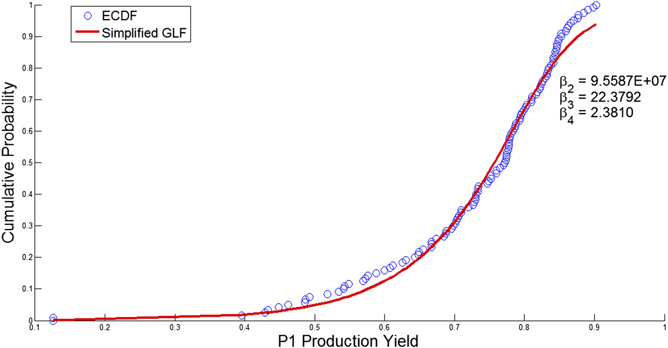
FIGURE 12. Distribution of the historical data for the production yield of facility P1 (Calfa et al., 2014).

When fitting the GLF to the empirical CDF data, the GLF can be simplified by setting ${\beta }_0=0$ and ${\beta }_1=1$ as these parameters correspond to the lower and upper asymptotes, respectively. The empirical CDF in Figure 12 can be approximated by the red GLF curve with ${\beta }_2=9.5587\times {10}^7$, ${\beta }_3=22.2792$, ${\beta }_4=2.3810$.

The NLP formulation that aims to match the moments, the covariances, and the distribution calculated from data is,

$\underset{x,p}{\text{min}}{z}_{\text{DMP}}^{L^2}={\displaystyle \sum _{i\in I}{\displaystyle \sum _{k\in K}{\text{w}}_{i,k}{\left(m_{i,k}-{\text{M}}_{i,k}\right)}^2}}+{\displaystyle \sum _{\underset{i<i^{\prime }}{\left(i,i^{\prime }\right)\in I}}{\text{w}}_{i,i^{\prime }}{\left(c_{i,i^{\prime }}-{\text{C}}_{i,i^{\prime }}\right)}^2}+{\displaystyle \sum _{i\in I}{\displaystyle \sum _{j=1}^N{\omega }_{i,j}{\delta }_{i,j}^2}}(\mathrm{14a})$

$\text{s}.\text{t}.\sum _{j=1}^N{p}_j=1(\mathrm{14b})$

$m_{i,1}=\sum _{j=1}^N{x}_{i,j}{p}_j\forall i\in I(\mathrm{14c})$

$m_{i,k}=\sum _{j=1}^N{\left(x_{i,j}-m_{i,1}\right)}^k{p}_j\forall i\in I,k>1(\mathrm{14d})$

$c_{i,i^{\prime }}=\sum _{j=1}^N\left(x_{i,j}-m_{i,1}\right)\left(x_{i^{\prime },j}-m_{i^{\prime },1}\right)p_j\forall \left(i,i^{\prime }\right)\in I,i<i^{\prime }(14e)$

$x_{i,j}\in \left[{\text{x}}_{i,j}^{\text{LB}},{\text{x}}_{i,j}^{\text{UB}}\right]\forall i\in I,j=1,\dots ,N(\mathrm{14f})$

$p_j\in \left[0,1\right]\forall j=1,\dots ,N(\mathrm{14g})$

$\widehat{\text{ECDF}}\left(x_{i,j}\right)-\stackrel{j}{{\displaystyle \sum }_{j\text{'}=1}}{p}_{j^{\text{'}}}={\delta }_{i,j}\forall i\in I,j=1,\dots ,N(\mathrm{14h})$

$x_{i,j}\le x_{i,j+1}\forall i\in I,j=1,\dots ,N-1(\mathrm{14i})$

where the entries of the uncertain parameters are indexed by $i\in I$. For example, if the uncertainties are the yields of some processes, I will be the set of these processes. N denotes the number of outcomes per node at the second stage, $j\in J=\left\{1,2,\dots ,N\right\}$ denotes the branches (outcomes) from the root node, and $k\in K=\left\{1,2,3,4\right\}$ is the index of the first four moments. The decision variables are the uncertain parameters of the stochastic programming problem, $x_{i,j}$, and their corresponding probabilities, $p_j$. The moments calculated from the tree are denoted by variables $m_{i,k}$ and the ones calculated from the data are denoted by parameters ${\text{M}}_{i,k}$. The covariances calculated between entity i and $i^{\prime }$ from the tree and the data are denoted by $c_{i,i^{\prime }}$ and $c_{i,i^{\prime }}$, respectively. Variables ${\delta }_{i,j}$ represent the deviations with respect to the empirical CDF data, which in turn are approximated by, for example, the GLF and is represented by the expression $\widehat{\text{ECDF}}\left(x_{i,j}\right)$. In addition to minimizing the weighted square errors from matching (co-)moments, the sum of squares of the deviations ${\delta }_{i,j}$ is also minimized with given weights ${\omega }_{i,j}$ that can be chosen relative to the weights for the term involving the moments.

Problem Eq. 14 minimizes the weighted Euclidean distance of the moments, covariances, and distribution from the scenario tree to those calculated from the data. Problem Eq. 14 is a nonconvex NLP because the variables x, m, and p are involved in the bilinear and trilinear terms in Eqs. 14d and 14e. If the empirical CDF is not considered, problem Eq. 14 reduces to the standard moment matching NLP problem proposed by Høyland and Wallace (2001).

7 Conclusion

We have provided an overview of stochastic programming in process systems engineering. The applications of stochastic programming are widespread, from the traditional petrochemical, pharmaceutical industry to carbon capture, energy storage. There are two major types of uncertainties that can be modeled using stochastic programming, exogenous uncertainty, which is the most commonly one considered, and endogenous uncertainty where realizations of the uncertainties depend on the decisions taken. Depending on the time discretization and the realizations of uncertainties, two-stage or multistage stochastic programming can be used to solve the problem under exogenous uncertainty. We have provided the mathematical formulations and algorithms for solving two-stage and multistage stochastic mixed-integer linear/nonlinear programming problems. Endogenous uncertainty is decision-dependent. Therefore, the scenario tree representation and the mathematical formulation of multistage stochastic programming under endogenous uncertainty differ from those of stochastic programming under exogenous uncertainty. To provide an intuitive view of the modeling framework, some process network design problems and a pooling problem are used as illustrative examples. Finally, we discussed how the scenario trees in stochastic programming can be generated from time-series models or historical data.

Despite the advances in applying stochastic programming in process systems, several challenges exist for its broader applications. First, it is often difficult to convince practitioners without any mathematical programming background to adopt stochastic programming methods in their problems. To that end, more tutorials and textbooks for practitioners rather than mathematicians need to be developed. Also, simulation can be used to verify the advantages of using stochastic programming. Second, the types of problems that can be solved efficiently are still limited. A utopia problem would be multistage stochastic mixed-integer nonlinear programming under both exogenous and endogenous uncertainty with an arbitrary probability distribution that can be stagewise dependent. The current algorithmic development and computational resources are still far from solving the utopia problem efficiently. The major challenge for algorithm development remains to be handling nonconvexity. Third, risk measures can be better integrated into stochastic programming, such as the ones used in chance-constrained programming. Other risk measures, such as Expected CVaR (conditional value at risk) (Pflug and Pichler, 2016), stochastic dominance (SD) (Ruszczyński, 2010), can also be used. Fourth, the connections of stochastic programming with the other 14 communities of decision-making under uncertainty (Powell, 2016) can be better established. Last but not least, generating a scenario tree that has a low error in practice requires high fidelity historical data and better forecast methods. The recent popularity and advances in data science and machine learning bring opportunities toward this direction.

Author Contributions

Both CL and IG designed the outline and the content of this manuscript. CL finished the writing of this manuscript under the guidance of Ignacio Grossmann.

Funding

This research was conducted as part of the Institute for the Design of Advanced Energy Systems (IDAES) with funding from the Simulation-Based Engineering, Crosscutting Research Program of the U.S. Department of Energy’s Office of Fossil Energy.

Conflict of Interest

The authors declare that the research was conducted in the absence of any commercial or financial relationships that could be construed as a potential conflict of interest.

Supplementary Material

The Supplementary Material for this article can be found online at: https://www.frontiersin.org/articles/10.3389/fceng.2020.622241/full#supplementary-material.

References

Acevedo, J., and Pistikopoulos, E. N. (1998). Stochastic optimization based algorithms for process synthesis under uncertainty. Comput. Chem. Eng. 22, 647–671. doi:10.1016/s0098-1354(97)00234-2

CrossRef Full Text | Google Scholar

Apap, R. M., and Grossmann, I. E. (2017). Models and computational strategies for multistage stochastic programming under endogenous and exogenous uncertainties. Comput. Chem. Eng. 103, 233–274. doi:10.1016/j.compchemeng.2016.11.011

CrossRef Full Text | Google Scholar

Beale, E. M. L. (1955). On minimizing a convex function subject to linear inequalities. J. Roy. Stat. Soc. B. 17, 173–184. doi:10.1111/j.2517-6161.1955.tb00191.x

CrossRef Full Text | Google Scholar

Birge, J. R. (1985). Decomposition and partitioning methods for multistage stochastic linear programs. Oper. Res. 33, 989–1007. doi:10.1287/opre.33.5.989

CrossRef Full Text | Google Scholar

Birge, J. R., and Louveaux, F. (2011). Introduction to stochastic programming. Heidelberg, Germany: Springer Science & Business Media.

Google Scholar

Boland, N., Dumitrescu, I., Froyland, G., and Kalinowski, T. (2016). Minimum cardinality non-anticipativity constraint sets for multistage stochastic programming. Math. Program. 157, 69–93. doi:10.1007/s10107-015-0970-6

CrossRef Full Text | Google Scholar

Bonami, P., Salvagnin, D., and Tramontani, A. (2020). “Implementing automatic Benders decomposition in a modern MIP solver,” in International conference on integer programming and combinatorial optimization, Heidelberg, Germany: Springer, 78–90.

CrossRef Full Text | Google Scholar

Calfa, B. A., Agarwal, A., Grossmann, I. E., and Wassick, J. M. (2014). Data-driven multi-stage scenario tree generation via statistical property and distribution matching. Comput. Chem. Eng. 68, 7–23. doi:10.1016/j.compchemeng.2014.04.012

CrossRef Full Text | Google Scholar

Cao, Y., and Zavala, V. M. (2019). A scalable global optimization algorithm for stochastic nonlinear programs. J. Global Optim. 75, 393–416. doi:10.1007/s10898-019-00769-y

CrossRef Full Text | Google Scholar

Christian, B., and Cremaschi, S. (2015). Heuristic solution approaches to the pharmaceutical R&D pipeline management problem. Comput. Chem. Eng. 74, 34–47. doi:10.1016/j.compchemeng.2014.12.014

CrossRef Full Text | Google Scholar

Chu, Y., and You, F. (2013). Integration of scheduling and dynamic optimization of batch processes under uncertainty: two-stage stochastic programming approach and enhanced generalized benders decomposition algorithm. Ind. Eng. Chem. Res. 52, 16851–16869. doi:10.1021/ie402621t

CrossRef Full Text | Google Scholar

Colvin, M., and Maravelias, C. T. (2008). A stochastic programming approach for clinical trial planning in new drug development. Comput. Chem. Eng. 32, 2626–2642. doi:10.1016/j.compchemeng.2007.11.010

CrossRef Full Text | Google Scholar

Dantzig, G. B. (1955). Linear programming under uncertainty. Manag. Sci. 1, 197–206. doi:10.1287/mnsc.1.3-4.197

CrossRef Full Text | Google Scholar

Ding, L., Ahmed, S., and Shapiro, A. (2019). A python package for multi-stage stochastic programming. Optimization online, 1–41.

Google Scholar

Dowson, O., and Kapelevich, L. (2020). SDDP.jl: a Julia package for stochastic dual dynamic programming. Inf. J. Comput. doi:10.1287/ijoc.2020.0987

CrossRef Full Text | Google Scholar

Escudero, L. F., Garín, M. A., and Unzueta, A. (2017). Scenario cluster lagrangean decomposition for risk averse in multistage stochastic optimization. Comput. Oper. Res. 85, 154–171. doi:10.1016/j.cor.2017.04.007

CrossRef Full Text | Google Scholar

Escudero, L. F., and Monge, J. F. (2018). On capacity expansion planning under strategic and operational uncertainties based on stochastic dominance risk averse management. Comput. Manag. Sci. 15, 479–500. doi:10.1007/s10287-018-0318-9

CrossRef Full Text | Google Scholar

Escudero, L. F., Monge, J. F., and Rodríguez-Chía, A. M. (2020). On pricing-based equilibrium for network expansion planning. a multi-period bilevel approach under uncertainty. Eur. J. Oper. Res. 287, 262–279. doi:10.1016/j.ejor.2020.03.048

CrossRef Full Text | Google Scholar

Gassmann, H. I., and Schweitzer, E. (2001). A comprehensive input format for stochastic linear programs. Ann. Oper. Res. 104, 89–125. doi:10.1023/a:1013138919445

CrossRef Full Text | Google Scholar

Gebreslassie, B. H., Yao, Y., and You, F. (2012). Design under uncertainty of hydrocarbon biorefinery supply chains: multiobjective stochastic programming models, decomposition algorithm, and a comparison between cvar and downside risk. AIChE J. 58, 2155–2179. doi:10.1002/aic.13844

CrossRef Full Text | Google Scholar

Geoffrion, A. M. (1972). Generalized benders decomposition. J. Optim. Theor. Appl. 10, 237–260. doi:10.1007/bf00934810

CrossRef Full Text | Google Scholar

Goel, V., and Grossmann, I. E. (2006). A class of stochastic programs with decision dependent uncertainty. Math. Program. 108, 355–394. doi:10.1007/s10107-006-0715-7

CrossRef Full Text | Google Scholar

Goel, V., and Grossmann, I. E. (2004). A stochastic programming approach to planning of offshore gas field developments under uncertainty in reserves. Comput. Chem. Eng. 28, 1409–1429. doi:10.1016/j.compchemeng.2003.10.005

CrossRef Full Text | Google Scholar

Grossmann, I. E. (2021). Advanced optimization for process systems engineering. in Cambridge series in chemical engineering. (Cambridge, England: Cambridge University Press.

Google Scholar

Guignard, M. (2003). Lagrangean relaxation. Top. 11, 151–200. doi:10.1007/bf02579036

CrossRef Full Text | Google Scholar

Guillén-Gosálbez, G., and Grossmann, I. E. (2009). Optimal design and planning of sustainable chemical supply chains under uncertainty. AIChE J. 55, 99–121. doi:10.1002/aic.11662

CrossRef Full Text | Google Scholar

Gupta, A., and Maranas, C. D. (2003). Managing demand uncertainty in supply chain planning. Comput. Chem. Eng. 27, 1219–1227. doi:10.1016/s0098-1354(03)00048-6

CrossRef Full Text | Google Scholar

Han, J.-H., and Lee, I.-B. (2012). Multiperiod stochastic optimization model for carbon capture and storage infrastructure under uncertainty in co2 emissions, product prices, and operating costs. Ind. Eng. Chem. Res. 51, 11445–11457. doi:10.1021/ie3004754

CrossRef Full Text | Google Scholar

Hart, W. E., Laird, C. D., Watson, J.-P., Woodruff, D. L., Hackebeil, G. A., Nicholson, B. L., et al. (2017). Pyomo-optimization modeling in python. Heidelberg, Germany: Springer.

CrossRef Full Text | Google Scholar

Hellemo, L., Barton, P. I., and Tomasgard, A. (2018). Decision-dependent probabilities in stochastic programs with recourse. Comput. Manag. Sci. 15, 369–395. doi:10.1007/s10287-018-0330-0

CrossRef Full Text | Google Scholar

Høyland, K., and Wallace, S. W. (2001). Generating scenario trees for multistage decision problems. Manag. Sci. 47, 295–307 47,295–307. doi:10.1287/mnsc.47.2.295.9834

CrossRef Full Text | Google Scholar

Kannan, R. (2018). Algorithms, analysis and software for the global optimization of two-stage stochastic programs. Ph.D. thesis, Massachusetts, MA: Massachusetts Institute of Technology.

Google Scholar

Karuppiah, R., and Grossmann, I. E. (2008). Global optimization of multiscenario mixed integer nonlinear programming models arising in the synthesis of integrated water networks under uncertainty. Comput. Chem. Eng. 32, 145–160. doi:10.1016/j.compchemeng.2007.03.007

CrossRef Full Text | Google Scholar

Kaut, M. (2011). Scenario generation for stochastic programming introduction and selected methods. SINTEF Technology and Society. 3, 1–61.

Google Scholar

Kaut, M., and Wallace, S. W. (2003). Evaluation of scenario-generation methods for stochastic programming. Yokohama, Japan: Yokohama.

Google Scholar

Kim, J., Realff, M. J., and Lee, J. H. (2011). Optimal design and global sensitivity analysis of biomass supply chain networks for biofuels under uncertainty. Comput. Chem. Eng. 35, 1738–1751. doi:10.1016/j.compchemeng.2011.02.008

CrossRef Full Text | Google Scholar

Kim, K., and Zavala, V. M. (2018). Algorithmic innovations and software for the dual decomposition method applied to stochastic mixed-integer programs. Math. Prog. Comp. 10, 225–266. doi:10.1007/s12532-017-0128-z

CrossRef Full Text | Google Scholar

Kittrell, J., and Watson, C. (1966). Don’t overdesign process equipment. Chem. Eng. Prog. 62, 79.

Google Scholar

Kleywegt, A. J., Shapiro, A., and Homem-de-Mello, T. (2002). The sample average approximation method for stochastic discrete optimization. SIAM J. Optim. 12, 479–502. doi:10.1137/s1052623499363220

CrossRef Full Text | Google Scholar

Küçükyavuz, S., and Sen, S. (2017). Leading developments from INFORMS communities—an introduction to two-stage stochastic mixed-integer programming. Maryland, MD: INFORMS.

Google Scholar

Laporte, G., and Louveaux, F. V. (1993). The integer l-shaped method for stochastic integer programs with complete recourse. Oper. Res. Lett. 13, 133–142. doi:10.1016/0167-6377(93)90002-x

CrossRef Full Text | Google Scholar

Lappas, N. H., and Gounaris, C. E. (2016). Multi-stage adjustable robust optimization for process scheduling under uncertainty. AIChE J. 62, 1646–1667. doi:10.1002/aic.15183

CrossRef Full Text | Google Scholar

Lara, C. L., Siirola, J. D., and Grossmann, I. E. (2019). Electric power infrastructure planning under uncertainty: stochastic dual dynamic integer programming (sddip) and parallelization scheme. Optim. Eng. 21, 1243–1281. doi:10.1007/s11081-019-09471-0

CrossRef Full Text | Google Scholar

Legg, S. W., Benavides-Serrano, A. J., Siirola, J. D., Watson, J. P., Davis, S. G., Bratteteig, A., et al. (2012). A stochastic programming approach for gas detector placement using CFD-based dispersion simulations. Comput. Chem. Eng. 47, 194–201. doi:10.1016/j.compchemeng.2012.05.010

CrossRef Full Text | Google Scholar

Levis, A. A., and Papageorgiou, L. G. (2004). A hierarchical solution approach for multi-site capacity planning under uncertainty in the pharmaceutical industry. Comput. Chem. Eng. 28, 707–725. doi:10.1016/j.compchemeng.2004.02.012

CrossRef Full Text | Google Scholar

Li, C., Bernal, D. E., Furman, K. C., Duran, M. A., and Grossmann, I. E. (2020). Sample average approximation for stochastic nonconvex mixed integer nonlinear programming via outer-approximation. Optim. Eng. doi:10.1007/s11081-020-09563-2

CrossRef Full Text | Google Scholar

Li, C., and Grossmann, I. E. (2019a). A finite $$\epsilon $$-convergence algorithm for two-stage stochastic convex nonlinear programs with mixed-binary first and second-stage variables. J. Global Optim. 75, 921–947. doi:10.1007/s10898-019-00820-y

CrossRef Full Text

Li, C., and Grossmann, I. E. (2019b). A generalized Benders decomposition-based branch and cut algorithm for two-stage stochastic programs with nonconvex constraints and mixed-binary first and second stage variables. J. Global Optim. 75, 247–272. doi:10.1007/s10898-019-00816-8

CrossRef Full Text | Google Scholar

Li, C., and Grossmann, I. E. (2018). An improved L-shaped method for two-stage convex 0-1 mixed integer nonlinear stochastic programs. Comput. Chem. Eng. 112, 165–179. doi:10.1016/j.compchemeng.2018.01.017

CrossRef Full Text | Google Scholar

Li, P., Arellano-Garcia, H., and Wozny, G. (2008). Chance constrained programming approach to process optimization under uncertainty. Comput. Chem. Eng. 32, 25–45. doi:10.1016/j.compchemeng.2007.05.009

CrossRef Full Text | Google Scholar

Li, X., Armagan, E., Tomasgard, A., and Barton, P. I. (2011a). Stochastic pooling problem for natural gas production network design and operation under uncertainty. AIChE J. 57, 2120–2135. doi:10.1002/aic.12419

CrossRef Full Text | Google Scholar

Li, X., Tomasgard, A., and Barton, P. I. (2011b). Nonconvex generalized benders decomposition for stochastic separable mixed-integer nonlinear programs. J. Optim. Theor. Appl. 151, 425. doi:10.1007/s10957-011-9888-1

CrossRef Full Text | Google Scholar

Lima, R. (2010). Ibm ilog cplex-what is inside of the box?” in Proc. 2010 EWO seminar (Pittsburgh, PA: Carnegie Mellon University).

Google Scholar

Liu, M. L., and Sahinidis, N. V. (1996). Optimization in process planning under uncertainty. Ind. Eng. Chem. Res. 35, 4154–4165. doi:10.1021/ie9504516

CrossRef Full Text | Google Scholar

Liu, P., Pistikopoulos, E. N., and Li, Z. (2010). Decomposition based stochastic programming approach for polygeneration energy systems design under uncertainty. Ind. Eng. Chem. Res. 49, 3295–3305. doi:10.1021/ie901490g

CrossRef Full Text | Google Scholar

Lubin, M., and Dunning, I. (2015). Computing in operations research using julia. Inf. J. Comput. 27, 238–248. doi:10.1287/ijoc.2014.0623

CrossRef Full Text | Google Scholar

Ogbe, E., and Li, X. (2019). A joint decomposition method for global optimization of multiscenario nonconvex mixed-integer nonlinear programs. J. Global Optim. 75, 595–629. doi:10.1007/s10898-019-00786-x

CrossRef Full Text | Google Scholar

Oliveira, F., Gupta, V., Hamacher, S., and Grossmann, I. E. (2013). A lagrangean decomposition approach for oil supply chain investment planning under uncertainty with risk considerations. Comput. Chem. Eng. 50, 184–195. doi:10.1016/j.compchemeng.2012.10.012

CrossRef Full Text | Google Scholar

Paules, G. E., and Floudas, C. A. (1992). Stochastic programming in process synthesis: a two-stage model with minlp recourse for multiperiod heat-integrated distillation sequences. Comput. Chem. Eng. 16, 189–210. doi:10.1016/0098-1354(92)85006-t

CrossRef Full Text | Google Scholar

Pereira, M. V. F., and Pinto, L. M. V. G. (1991). Multi-stage stochastic optimization applied to energy planning. Math. Program. 52, 359–375. doi:10.1007/bf01582895

CrossRef Full Text | Google Scholar

Pflug, G. C., and Pichler, A. (2016). Time-consistent decisions and temporal decomposition of coherent risk functionals. Mathematics. 41, 682–699. doi:10.1287/moor.2015.0747

CrossRef Full Text | Google Scholar

Pistikopoulos, E. N., and Ierapetritou, M. G. (1995). Novel approach for optimal process design under uncertainty. Comput. Chem. Eng. 19, 1089–1110. doi:10.1016/0098-1354(94)00093-4

CrossRef Full Text | Google Scholar

Powell, W. B. (2016). Optimization challenges in complex, networked and risky systems—a unified framework for optimization under uncertainty. Maryland, MD: INFORMS.

Google Scholar

Powell, W. B. (2019). A unified framework for stochastic optimization. Eur. J. Oper. Res. 275, 795–821. doi:10.1016/j.ejor.2018.07.014

CrossRef Full Text | Google Scholar

Rockafellar, R. T., and Wets, R. J.-B. (1991). Scenarios and policy aggregation in optimization under uncertainty. Mathematics. 16, 119–147. doi:10.1287/moor.16.1.119

CrossRef Full Text | Google Scholar

Ruszczyński, A. (1997). Decomposition methods in stochastic programming. Math. Program. 79, 333–353. doi:10.1016/s0025-5610(97)00041-5

CrossRef Full Text | Google Scholar

Ruszczyński, A. (2010). Risk-averse dynamic programming for Markov decision processes. Math. Program. 125, 235–261. doi:10.1007/s10107-014-0783-z

CrossRef Full Text | Google Scholar

Sahinidis, N. V. (2004). Optimization under uncertainty: state-of-the-art and opportunities. Comput. Chem. Eng. 28, 971–983. doi:10.1016/j.compchemeng.2003.09.017

CrossRef Full Text | Google Scholar

Sand, G., and Engell, S. (2004). Modeling and solving real-time scheduling problems by stochastic integer programming. Comput. Chem. Eng. 28, 1087–1103. doi:10.1016/j.compchemeng.2003.09.009

CrossRef Full Text | Google Scholar

Sargent, R. (2005). Process systems engineering: a retrospective view with questions for the future. Comput. Chem. Eng. 29, 1237–1241. doi:10.1016/j.compchemeng.2005.02.008

CrossRef Full Text | Google Scholar

Shapiro, A., Dentcheva, D., and Ruszczyński, A. (2014). Lectures on stochastic programming: modeling and theory. Philadelphia, Pennsylvania: SIAM.

Google Scholar

Tarhan, B., and Grossmann, I. E. (2008). A multistage stochastic programming approach with strategies for uncertainty reduction in the synthesis of process networks with uncertain yields. Comput. Chem. Eng. 32, 766–788. doi:10.1016/j.compchemeng.2007.03.003

CrossRef Full Text | Google Scholar

Torres, J. J., Li, C., Apap, R. M., and Grossmann, I. E. (2019). A review on the performance of linear and mixed integer two-stage stochastic programming algorithms and software. Optimization Online.

Google Scholar

Van Slyke, R. M., and Wets, R. (1969). L-shaped linear programs with applications to optimal control and stochastic programming. SIAM J. Appl. Math. 17, 638–663. doi:10.1137/0117061

CrossRef Full Text | Google Scholar

Wallace, S. W., and Ziemba, W. T. (2005). Applications of stochastic programming. Philadelphia, Pennsylvania: SIAM.

Google Scholar

Watson, J.-P., Woodruff, D. L., and Hart, W. E. (2012). Pysp: modeling and solving stochastic programs in python. Math. Prog. Comp. 4, 109–149. doi:10.1007/s12532-012-0036-1

CrossRef Full Text | Google Scholar

Yang, Y., and Barton, P. I. (2016). Integrated crude selection and refinery optimization under uncertainty. AIChE J. 62, 1038–1053. doi:10.1002/aic.15075

CrossRef Full Text | Google Scholar

Ye, Y., Li, J., Li, Z., Tang, Q., Xiao, X., and Floudas, C. A. (2014). Robust optimization and stochastic programming approaches for medium-term production scheduling of a large-scale steelmaking continuous casting process under demand uncertainty. Comput. Chem. Eng. 66, 165–185. doi:10.1016/j.compchemeng.2014.02.028

CrossRef Full Text | Google Scholar

Zavala, V. M. (2014). Stochastic optimal control model for natural gas networks. Comput. Chem. Eng. 64, 103–113. doi:10.1016/j.compchemeng.2014.02.002

CrossRef Full Text | Google Scholar

Zeballos, L. J., Méndez, C. A., Barbosa-Povoa, A. P., and Novais, A. Q. (2014). Multi-period design and planning of closed-loop supply chains with uncertain supply and demand. Comput. Chem. Eng. 66, 151–164. doi:10.1016/j.compchemeng.2014.02.027

CrossRef Full Text | Google Scholar

Zeng, Z., Christian, B., and Cremaschi, S. (2018). A generalized knapsack-problem based decomposition heuristic for solving multistage stochastic programs with endogenous and/or exogenous uncertainties. Ind. Eng. Chem. Res. 57, 9185–9199. doi:10.1021/acs.iecr.8b00822

CrossRef Full Text | Google Scholar

Zeng, Z., and Cremaschi, S. (2018). Multistage stochastic models for shale gas artificial lift infrastructure planning. Computer aided chemical engineering. 44, 1285–1290.

CrossRef Full Text | Google Scholar

Zhang, Q., Cremer, J. L., Grossmann, I. E., Sundaramoorthy, A., and Pinto, J. M. (2016). Risk-based integrated production scheduling and electricity procurement for continuous power-intensive processes. Comput. Chem. Eng. 86, 90–105. doi:10.1016/j.compchemeng.2015.12.015

CrossRef Full Text | Google Scholar

Zou, J., Ahmed, S., and Sun, X. A. (2018). Multistage stochastic unit commitment using stochastic dual dynamic integer programming. IEEE Trans. Power Syst. 34, 1814–1823. doi:10.1109/TPWRS.2018.2880996

Google Scholar

Zou, J., Ahmed, S., and Sun, X. A. (2019). Stochastic dual dynamic integer programming. Math. Program. 175, 461–502. doi:10.1007/s10107-018-1249-5

CrossRef Full Text | Google Scholar