Curating and Visualizing Dense Networks of Monsoon Precipitation Data: Integrating Computer Science Into Forward Looking Climate Services Development

Introduction

The North American Monsoon (NAM) is a seasonal phenomenon characterized by increased precipitation driven by a shift in the mid-level circulation pattern across the western U.S. and subsequent increase in moisture availability in the Southwest U.S (Adams and Comrie, 1997; Higgins et al., 1997). The influx of low-level moisture conducive to support monsoon precipitation emerges and intensifies in late June and declines in late September (Douglas et al., 1993; Maddox et al., 1995). Previous attempts to characterize the monsoon used the progression of precipitation amounts and extent to identify the onset, persistence, and decline of monsoon related activity, while some local National Weather Service offices used dewpoint temperature thresholds to identify the onset of monsoon activity (Ellis et al., 2004). To aid in messaging and public outreach over seasonal hazards and to facilitate standardized comparisons of cumulative precipitation totals, the official National Weather Service definition of the monsoon was changed in 2008 to the period between June 15th and September 30th.

Single station metrics using a limited number of stations - typically a municipal airport or other long term National Weather Service stations - provide benchmarks that track the daily and cumulative totals for the monsoon during the aforementioned standardized seasonal window. This facilitates comparisons to long term averages and daily and seasonal records at these stations. Station level monsoon precipitation tracking stands in as approximations for the location of regional monsoon activity, allowing for intra- and inter-annual spatial and temporal comparisons, between geographies and years, respectively. Daily totals identify the broad outlines of regional variability by identifying where recent monsoon activity occurred, while the seasonal (annual monsoon) totals index each year against other years and climatology. Daily and seasonal totals are some of the primary metrics used to track the seasonal progression and rank of each year of the monsoon, while the impacts associated with extreme events are of great interest to emergency managers, planners, and flood control district analysts (Shoemaker and Davis, 2008; Demaria et al., 2019).

The inherent challenge in using stations from around the region to characterize the monsoon, is that monsoon precipitation shows considerable spatial and temporal variability at both the event and annual timescale, and within and across years (Mullen et al., 1998; Englehart and Douglas, 2006). On average, the monsoon is the source of up to half of the annual rainfall in the Southwest during this period (Crimmins, 2006), but any given seasonal total can vary considerably from the long term average. The manner in which these cumulative seasonal rainfall totals are achieved is highly variable in both timing and intensity. Some years have a lower number of days with rain but a few highly intense storm events, while other years have more frequent and regular rain (see Ellis et al., 2004).

Monsoon events (either single days or multi-day precipitation events) are frequently spatially heterogeneous in both precipitation extent and intensity within relatively small spatial bounds (Crimmins et al., 2021). The variability in intensity is especially relevant in urban areas as it relates to flood risk potential, where the location and intensity of storm activity can have dramatic effects, especially during the strongest of storms (Garcia et al., 2008; Crimmins et al., 2021). This variability makes characterizing the monsoon a challenge at local scales, given the steep gradients of spatial heterogeneity observed in single events or across seasonal totals. This variability is pronounced even at the finest scales, where a single monsoon event or runs of storms can produce concentrated and heavy precipitation in one location, while other locations within the same municipal area record much less (and sometimes zero) precipitation. This is sometimes described in local media reports as the “winners and losers” in a monsoon storm (see NWS El Paso, 2020), or lucky vs. unlucky when these patterns turn more intense, potentially dangerous, and occasionally deadly.

Daily and seasonal/annual totals at a single station are one way of tracking the progression and performance of the monsoon, but they do not capture fine scale spatial variability. During single days or across multi-day precipitation events, a single station is unlikely to be representative for the region, especially given the range of local variability often seen in monsoon precipitation. Additionally, precipitation measurements from official monitoring stations do not generally provide enough spatial coverage in a region to capture small events or steep gradients of precipitation variability. Gridded estimates of precipitation provide full coverage of the region. They range in spatial resolution from 1 km (MRMS) to 4 km (PRISM) for freely available products, while 800 m (PRISM) data is available for a fee. Despite offering comprehensive coverage of the region, these gridded products still may not capture the spatial variability in precipitation even at the resolution at which the data are provided, and small events or those with steep gradients in precipitation intensity are not always well-captured by these data. This inability to capture and characterize variability, and overall lack of access to finer resolution data highlights a gap in regional climate services. Information about the spatial variability and range of intensity of storm events would be useful across a range of decision making contexts. This includes flood control and emergency management (Zanchetta and Coulibaly, 2020), phenology and invasive species green-up (Wallace et al., 2016), and irrigation control and water use decisions (Goap et al., 2018).

One solution to this lack of appropriately scaled data is development-of, or opportunistic sampling-from, dense networks of precipitation monitoring stations located within a municipal area. There are emergent research efforts to use dense networks to better characterize variability in monsoon precipitation (Demaria et al., 2019; Crimmins et al., 2021), some of which provide dozens or even hundreds of additional stations as a supplement to official stations. On the applications side, flood control districts already use automated sensors to track precipitation events for flood risk assessment and monitoring. Other sources are also available, including NOAA-COOP, Mesowest, citizen science monitoring data (e.g., CoCoRaHS and Rainlog) and gridded-interpolated or radar-derived estimates (such as PRISM or MRMS). A mix of these data are already in use in an ad hoc manner by both researchers and decision makers to describe monsoon events, especially larger impact events shortly after they occur.

These networks of station data are useful for analyzing monsoon events. Their density, especially when multiple networks are used in tandem, begin to capture some of the variability of smaller monsoon precipitation events. There are a few challenges for using these networks of sensors: (1) they derive from multiple sources with different mechanisms for presenting or giving access to the data, and (2) they record data over different windows of time. Assessments of these networks and their timing identified the varying windows of date attribution for the different networks (Figure 1; note the dates listed on this figure were how we documented the challenges in temporal attribution using a specific date that illustrated the variable timing of the different networks). This highlights the challenge of integrating data that was captured on either calendar date (midnight to midnight) or another temporal window (12z−12z, etc.). Integrating these data into decision making contexts or research applications poses an inherent data management challenge for processing and analyzing data from these sources. To date, there is not a singular platform that organizes these data in an accessible way.

FIGURE 1

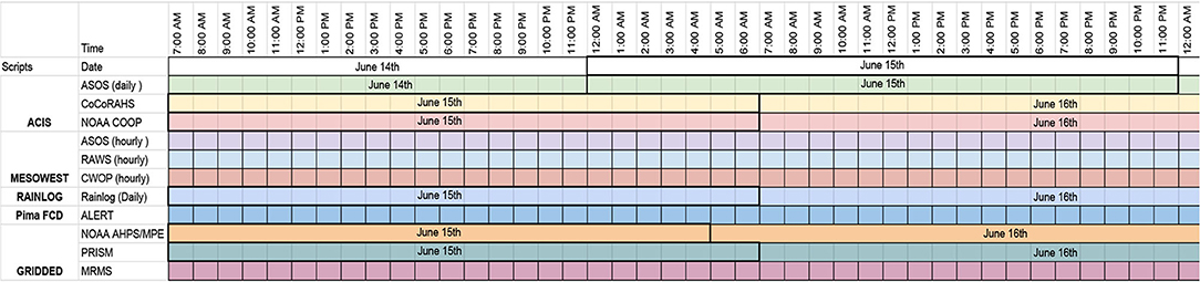
Figure 1. Date and timing windows for station based observations and gridded precipitation estimates.

This project originated based on our own use of these data, and our observation that others in the regional stakeholder and collaborator network were using these data in an opportunistic way. This included daily precipitation summaries, examples of precipitation variability within the metropolitan region, or in identifying regions with possible-to-likely flooding impacts. We felt that a central repository that brought together these data sources would be useful for our own research and climate services development, and would also serve as a value-add to stakeholders in our network (cf. Mahmood et al., 2017) who were grappling with similar or related questions about monsoon variability. We also hoped this would also serve a bridging function (see boundary objects/organizations: Lemos et al., 2014) that brought together new partnerships or collaborations centered on the use of these aggregated data. We developed a platform that allowed for visualization-of and access-to these data.

We recognized the complexity of aggregating data from multiple sources, developing a workflow to manage and store these data, and the need for a robust visualization platform using these data. This was a computer science and data management driven challenge as much as it was a question of climate services development. This helped catalyze activity in our UArizona research computing working group. This group, located within the Arizona Institutes for Resilience (AIR) is focused on research collaboration and technology development at the intersection of natural, social, and computer sciences. The monsoon variability provided a reason, and computer science and cloud computing techniques provided a mechanism, to collaborate across disciplines to address the computational and data-organizational challenges of scraping, querying, and visualizing these data in a way not previously possible via ad hoc use-of or access-to the data. We also prototyped an Application Programming Interface (API) for eventual use by stakeholders interested in accessing the data stored and visualized in this platform. An API is a programmatic interface developed to allow requests to an external application or data set. An API enables users to send or receive data dependent on the API's intended design and function.

In this paper, we present the process by which we aggregated and organized precipitation data from multiple sources. We summarize the development of a web based data visualization tool that synthesizes and visualizes station based precipitation monitoring data in conjunction with MRMS derived gridded estimates of precipitation. Our initial goal was to develop a monsoon event-viewer for use in visualizing and analyzing monsoon variability after daily or multi-day events. We added database and API development to facilitate data access both within our stakeholder network on partnered projects and outside this network via API access. We present a climate services-motivated question and posit that access to increasingly granular data about monsoon precipitation events using a computer science informed approach adds value in the climate services context and demonstrates what a collaborative project between these fields looks like. In the following sections we outline the process by which we aggregated and organized the data and describe what the monsoon event viewer looks like in practice. We also discuss preliminary analyses of monsoon activity using these data. We conclude with a discussion of the potential-for and limitations-of collaborations between climate services and computer science. This includes application development and directions for future work.

Materials and Methods

The framework for this project emerged during our own initial attempts to collect and organize data from various sources and sensors around the region. We identified and summarized the data sources, including information about their window of data capture and approximate availability, and developed a preliminary scraping schema for some of the data. This process was not systematic or easily replicable, and was limited to our opportunistic samples of data based on what was easily obtainable. This made clear the need for a strategy to organize, analyze, and visualize these data, and is a major reason we expanded our team to include computer science and application development expertise.

The following section gives a plain language overview of the technical steps involved in this process. We start with the overall structure and architecture of the platform and database architecture, before we provide additional details on each of the relevant steps in building the database, organizing the data, and developing the web-based visualization platform. This section outlines technical challenges, and the solutions we employed in each step of the platform development process. We also briefly describe preliminary case study analyses we used as a test run for the platform, before moving on to the results of these tests. In the discussion section we further address challenges and opportunities of bringing together computer science expertise and climate services development.

Data Collection

Overview and Database Architecture

This section includes technical information about the development of the database architecture, the data scraping and organization schema, and the backend database and frontend web visualization technologies. It is presented to document the steps to replicate or adapt these processes. For those interested in the monsoon viewer but not the mechanisms that built it, we suggest skipping to section Results.

One of the first challenges faced was developing an automated and repeatable process for gathering and storing rainfall data. We had multiple flood control district (FCD) and rainfall data sources independently run by the state of Arizona, individual counties in Arizona, and research programs. We organized these data sources into networks which we named Pima FCD, Maricopa FCD, Rainlog, Mesowest, and State FCD. The database containing the sensor data for each network is housed within an Amazon Web Services (AWS) service called Relational Database Service (RDS). RDS is Amazon's scalable cloud-based hosting solution with multiple database engine offerings and can be optimized for memory or read/write performance. This project utilizes the MariaDB engine which is an open source relational database engine from the developers of MySQL (see glossary for details on the various referenced technologies). The database contains a total of 10 tables. Each network requires two tables for housing sensor metadata and rainfall readings. The metadata table consists of latitude and longitude coordinate locations, the date the sensor first came online, a unique sensor ID, a name which is usually relevant to its geographic location, and sensor type. Figure 2 is a screen capture that displays architecture details of the metadata table. Rainlog, a self-report citizen science network, has a slightly different metadata architecture that incorporates a revision_id field. In the event a Rainlog user moves, this field is used to associate users back to their original sensor_id field with new latitude and longitude location. The table details are found in the screen capture in Figure 3. The sensor readings table contains the rainfall reading data from each sensor in each network. The database structure consists of a primary key reading_id, sensor_id that is a foreign key to the metadata table sensor_id, the reading_value the sensor reported, reading_date, reading_time, and if the data is considered anomalous for the network value. Figure 4 is a screen capture that includes the details for the sensor readings table.

FIGURE 2

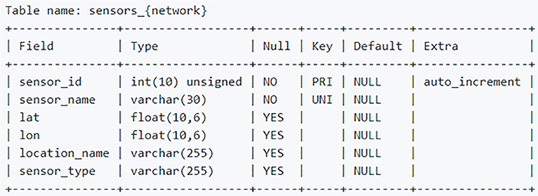
Figure 2. Database architecture of the main metadata table.

FIGURE 3

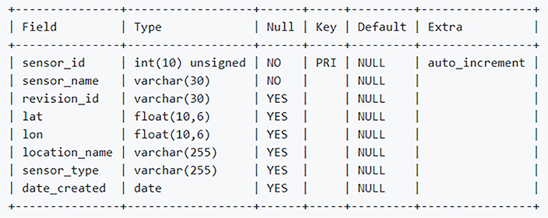
Figure 3. Database architecture of the rainlog metadata table.

FIGURE 4

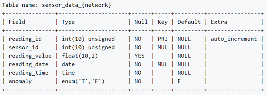
Figure 4. Database architecture of the sensor readings table.

Discovery

While investigating the public frontend websites of the networks, we found the county and state FCD networks were utilizing the same commercial product. This commercial product gathers and stores readings from the remote sensors located throughout each network's monitoring region and has a built-in frontend web interface used to present the data on county or state-maintained websites. The challenge in gathering the data from the state and county sensor networks is each was technically implemented in a different manner from the next while still being an implementation of the same underlying commercial product. We also discovered that the state FCD network lacks a public API that could have been used to make programmatic calls from various programming languages to gather data. Whereas, Rainlog and Mesowest both have APIs we query for data (note: we integrated data from the Mesowest repository using the SynopticsLabs API).

Data Scraping

From our discovery process we learned the only way to source the data for the state and county sensor networks was through their web frontends since they lack an API. Through these frontends we programmatically identified individual sensors on a per network basis. We then created database tables per network containing metadata for each network's sensors. These tables contain data such as unique sensor IDs, latitude and longitude coordinates, and when a sensor first came online. We then use these network tables to programmatically iterate through each identified sensor to gather reading values from the sensor's specific web frontend. In order to gather that rainfall reading data, we utilize Python and a module called BeautifulSoup. We identify the relevant elements that make up the web frontend of each sensor's specific readings page such as reading values, date, time, and if the sensor detected an anomaly in the reading value. Python and BeautifulSoup then programmatically scrapes that data and stores it in our RDS MariaDB instance. This process repeats per sensor in each network table for Pima FCD, Maricopa FCD, and State FCD.

In addition to developing a data scraping solution for the county and state networks, we also discovered the frequency at which we gathered the data was important. The Maricopa FCD network would return a daily total per sensor for the previous day without incremental readings throughout the day. We found if we scraped the data every 60 minutes, we would capture incremental readings every 15 min. This is important to understanding rainfall frequency in certain areas of the network's geographic region. The Pima FCD network reported at varying frequencies depending on which sensors detected rainfall. A typical reporting frequency during a rainfall event was every 5 min. We find this reporting frequency important because of the opportunity it provides to perform a near real-time analysis of the readings. The flexibility of the AWS platform allows us to run our Lambda scripts at user defined frequencies. This means we could gather rainfall data at faster intervals for more immediate data processing such as predictive modeling for severe weather events or flooding.

Gathering data from the Rainlog and Mesowest networks was a different process because both have APIs in place that allow for data to be requested directly from the network. This is done by creating an account with the network and requesting an API key, which in turn allows for request calls to be made directly from a Python script. Rainlog required two different calls to be made. One of them was to request all revision IDs within a given region. A region is defined by drawing a shape between latitude and longitude points. Since Rainlog allows users to move locations and keep the same account, revision IDs represent a way to track the latest sensor ID, along with its latest location. After the call to request revision IDs is made, a second call is made to request rainfall data for all sensors in a region using a date range as a parameter. Mesowest worked in a similar way, where a region is defined, and rainfall data was requested for a certain date range. The main difference was that stations did not change location and there was no need to make multiple calls. Finally, after the Lambda functions run for each of these two networks, the data obtained is then added to a MariaDB database within RDS.

Data Visualization

The intention of the data visualization is to aggregate the collected data and model it in a meaningful manner while providing a straightforward user experience. This is done in two phases, the backend API, and the web application frontend. These phases make use of an S3 Static Web Hosting Bucket, an EC2 Instance virtual machine, and an RDS MariaDB database all provided by AWS used in tandem as shown by the control-flow diagram in Figure 5.

FIGURE 5

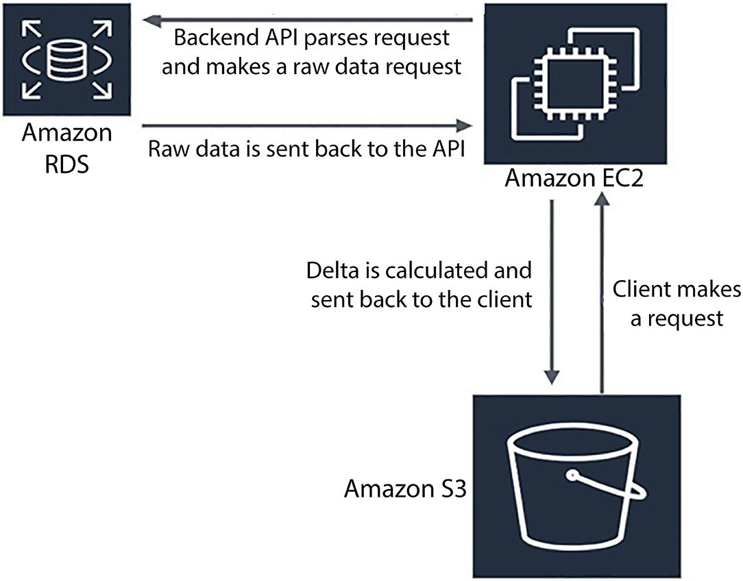
Figure 5. Amazon web services control flow diagram.

Backend API

The backend API serves as a control center for the entire data visualization application. Built with Node.js using the Express framework, the API will accept RESTful queries detailing (1) what network is to be shown, (2) what date or date range, (3) and whether MRMS gridded data is to be returned. Supplementary Table 1 lists the services and versions used to create the backend API.

During a query in which MRMS data is not requested, the API will make a query to the AWS RDS database for the user selected dates and networks. When the data is delivered back to the API it is in a raw format and represents how much rainfall a sensor has collected at the time of reporting. This is the case for the Pima FCD, Maricopa FCD, State FCD, and Mesowest networks. The Rainlog network is a special case as the reported values are how much it had rained for that 24-h period. Once this raw data is retrieved it is filtered, formatted, and a delta calculation will be performed (Pima FCD, Maricopa FCD, State FCD and Mesowest) resulting in the amount of precipitation that fell for the requested period. During this stage, specifically the delta calculation for the FCD networks, special conditionals will look for any anomalous readings that may be in the data. This check on the readings delta was only in place for the FCD stations, as the other networks presumably have their own QA/QC measures. Anomalous data for the FCD networks are counted as any two readings whose change results in a negative value (i.e., the sensor tipped over to empty its' collection tank) or the change results in a value greater than a specified threshold. We reviewed historical records for the FCD networks, which revealed large delta errors were exceedingly rare, and in some cases, preceded instances where the sensor was taken offline for repairs or stopped recording altogether. The threshold value was designed to filter out extreme readings that were due to clear and obvious errors in the data or sensor operation. A comprehensive review of the different networks is outside the scope of this paper, but we are working on an analysis that assesses the different station networks, so as to better understand their observations in comparison to other networks, as well as to gridded estimates of precipitation.

After all the data has been formatted, filtered, and the delta calculation has been performed, the API will then merge each sensor's rainfall data with its geospatial data. The geospatial data is collected from a cronjob executing at 12:00 UTC daily, which is then written to a specific file contained locally on the AWS EC2 Instance. At this stage the data has been formatted in an array of JSON objects, where each JSON object contains the precipitation amount, the sensor name, and the latitude and longitude for each sensor which is then sent back to the web application frontend.

The MRMS data retrieval and processing are a separate process from a network precipitation query as described above. A cronjob executed daily at 12:00 UTC calls a Python script which (1) retrieves a raw binary GRIB2 file from the MRMS website, (2) crops a bounding box around Arizona and New Mexico, (3) converts the GRIB2 file to a readable NumPy array using PyGrib, (4) names and stores a compressed NumPy array file representing the rainfall for the previous day's 24-h period from 5:00 a.m. to 5:00 a.m. Arizona time. On a request for MRMS data from the web frontend, similar to a network precipitation request, the Node.js API will accept and parse the request, yet it will then execute a Python script detailing the request day for the MRMS data. This Python script will (1) read the compressed NumPy array (which contains point data 4 km apart from each other with geospatial data in a Web Mercator mapping), (2) convert each Web Mercator point into a latitude and longitude, (3) and write an array of JSON objects that is then sent back to the web frontend.

On any given day, the EC2 Instance stores the past week of MRMS data locally in its compressed NumPy array format, and the current day's MRMS data in an array of JSON objects that is readable by the web frontend. This is done as a “storage safe saving solution” as the compressed NumPy arrays range from 4 to 5 MB while the uncompressed array of JSON objects on average range from 50 to 55 MB in size. The theory is that a user is more likely to look at the current day's MRMS data than a historical date, therefore, the backend API can send the file on demand rather than processing a historical MRMS file which in turn takes more compute time.

Frontend Web Application

The intention of the frontend is to visualize the data in a meaningful manner while providing a straightforward user experience. This is done by utilizing the React Framework where a component-based paradigm is used, such that every element in the DOM (Document Object Model) can be represented as a React “component.” All these components are then compiled in a hierarchal manner into one main “parent” component which represents the overall webpage. Supplementary Table 2 is the complete list of dependencies that the React application utilizes.

The main component of the webpage is built using the Deck.gl data visualization library. Our Deck.gl component uses a base layer of a static Web Mercator map (provided by the MapBox API) and a default “icon layer” visible when the webpage is loaded. This layer uses symbolic representation to display (1) how much precipitation each sensor received (via its color) and (2) which network the sensor belongs to (via its symbol). This data is collected via HTTPS requests to the backend API specifying what date/date range and what networks to display. By default, the web application will make a request for the Pima FCD network's data for the day before upon a user visiting the website. Any other request for either MRMS or another network's data will be a separate HTTPS request to the backend.

Before the React application is sent to AWS S3 for hosting, the application will go through a compiling process to improve the overall performance of the website. This process is done by React's build feature. The build process will (1) use the transcompilier Babel to convert the ECMAScript 2016 (ES6) JavaScript into a version that is compatible with all web browsers, and (2) combine all the separate JavaScript components and Cascading Style Sheets (CSS) into one single file. Combining the JavaScript and CSS will allow the client to make less HTTPS requests upon loading the webpage. Once the build process has finished, the compiled built application will be uploaded to an AWS S3 Bucket configured for static web hosting using the “AWS Sync” function on the AWS CLI (Command Line Interface).

Testing the Monsoon Visualizer

To test the utility of the monsoon viewer and database/API, we used a case study examples to illustrate events where the database/viewer is well-suited to capture precipitation variability not well-characterized elsewhere. We also used maps of annual totals, plots of the range of variability across these totals, and inter-annual comparisons to briefly illustrate how further exploration of the database/API could look to monthly or seasonal typologies of monsoon activity. In the results below, we present these examples of how snapshots of daily or event data (maps and plots), along with seasonal summaries and inter-annual comparison plots, can all illustrate various temporal scales of monsoon variability. In the discussion we speak to possible applications of these data.

Results

The results we present here demonstrate the strength of systematic aggregation of monsoon data, as well as the utility of making these data available in an intuitive/visual platform. This aggregated data captures aspects of monsoon variability that are not represented by single station metrics, and analysis and visualization of these data is not easily possible without a centralized database and visualization platform. The monsoon viewer itself is live at monsoon.environment.arizona.edu. Version 1.0 of the viewer includes daily precipitation totals from the Pima and Maricopa Flood Control District sensor networks, Mesowest, and Rainlog. The viewer also includes MRMS/radar derived estimates of precipitation for the previous seven days. Data visualization options include selection of one or more of the station networks, summarization of these data via a heat map and hex map visualization function, and MRMS gridded data (for the previous seven days). All data presented in the viewer are available for download as a CSV file that contains the coordinates of the station, the name of the network and sensor, and the daily total precipitation for the date specified.

Exploring Recent Precipitation Events With the Monsoon Viewer

In early July 2018, heavy and localized rain to the northwest of Tucson (but within the Tucson Metropolitan region) caused intense localized flooding and a train derailment. Over a 3-day period station totals in the Tucson Metropolitan area ranged from over 7 inches to at or near zero (Figure 6), while the Tucson International Airport (the National Weather Service station used for long term statistics and monitoring), recorded 0.09 inches over the same 3 day window. This event highlights the extreme variability that can be observed over a single day or short run of days during the monsoon (note: the single day totals for July 8 and July 10 exhibit similar variability). This also highlights events where antecedent conditions could help inform decision making and planning. The single day totals were impressive, but flood risk is also linked to cumulative conditions when multiple intense events stack up, particularly when they hit the same locations.

FIGURE 6

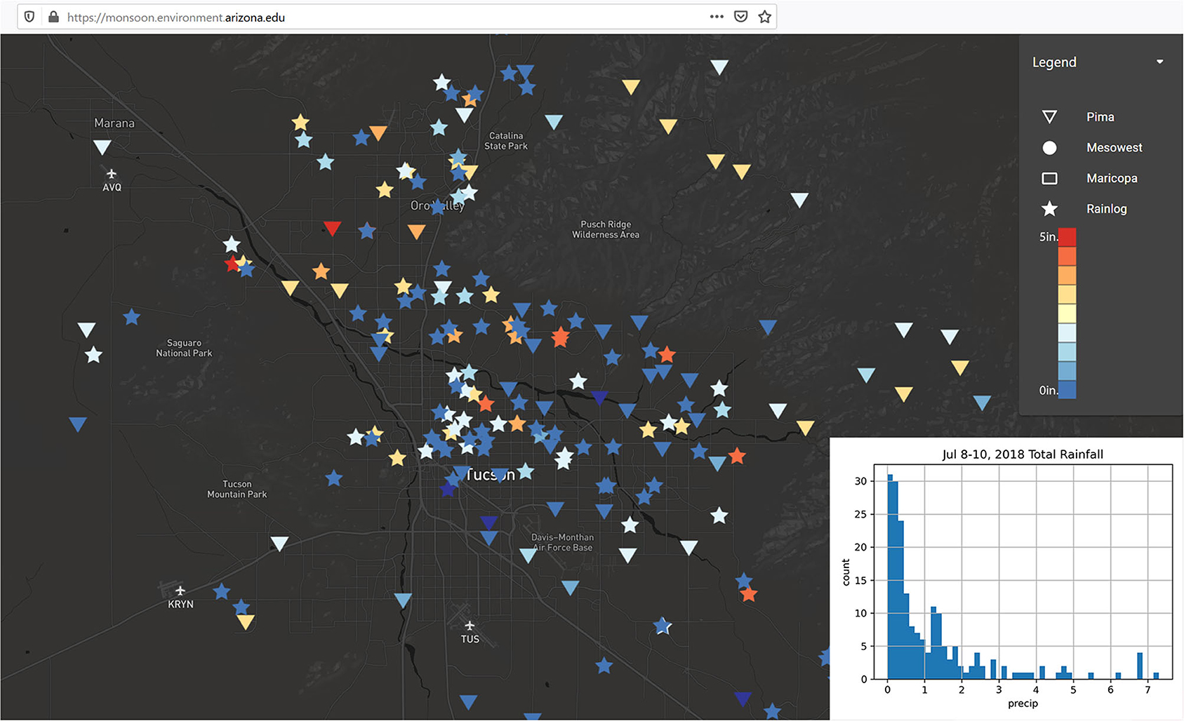
Figure 6. Tucson Metropolitan Region Total Precipitation - Jul 8-10, 2018 - Highly Variable Cumulative 3 Day Totals.

In July 2020, a much more widespread precipitation event was notable for the intense precipitation that fell across a larger swath of the city (Figure 7), along with the steep gradient as precipitation levels dropped off. A mere 0.15″ of precipitation fell at the Tucson International Airport station, which is ~10 miles away from the station that recorded the highest daily total. Note there are a small number of events in the period of record when the airport receives at or near the highest daily total; even when much of the city sees little precipitation. This is not meant to question the use of the airport as a standard metric, but merely to illustrate what a fine-grained data viewer can capture, especially at the daily or event timescale.

FIGURE 7

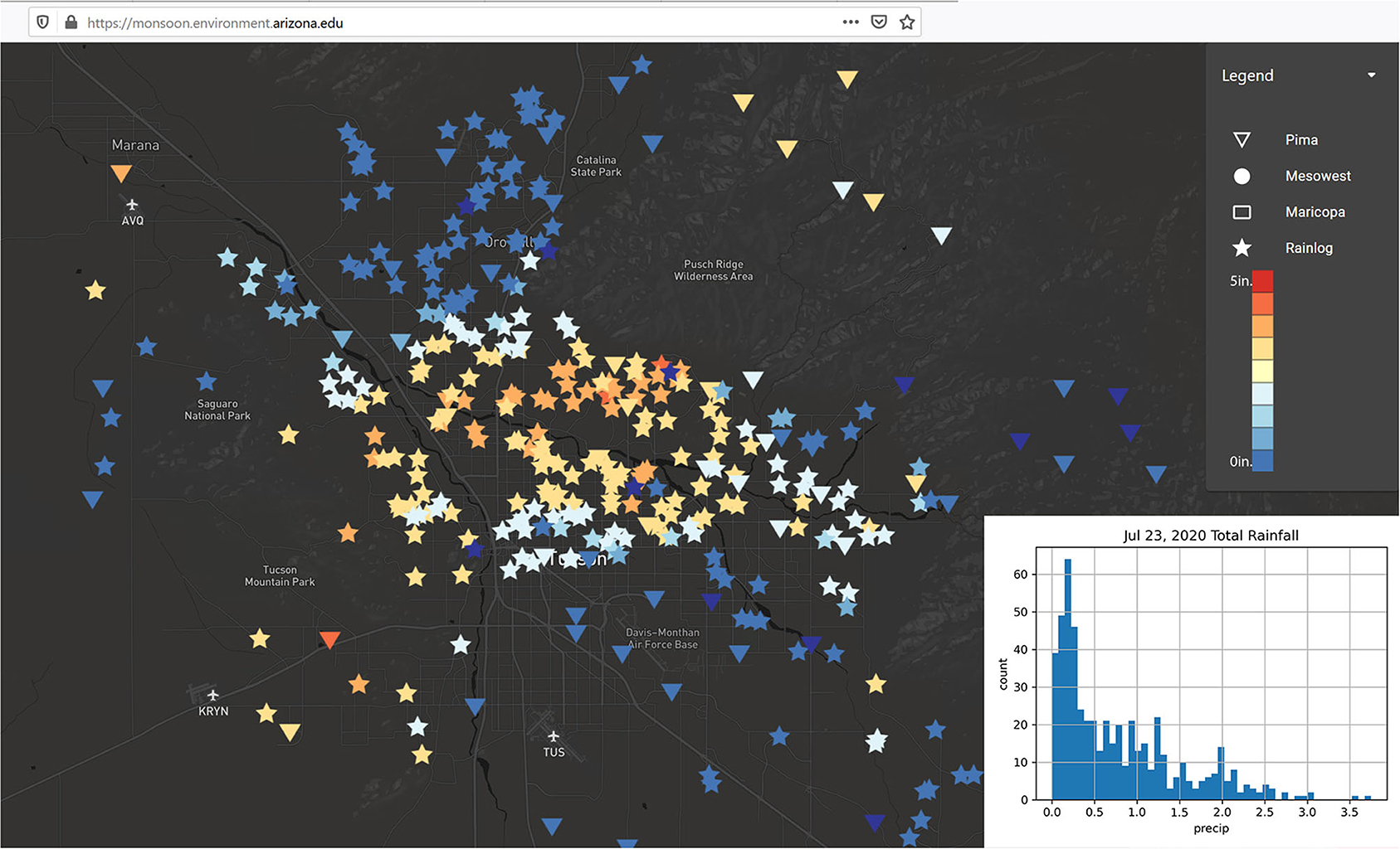
Figure 7. Tucson Metropolitan Region Total Precipitation - Jul 23, 2020 - Widespread Event with Steep Dropoffs in Total Precipitation.

This widespread activity on July 23 is also a good example of a few of the beta features in the monsoon viewer – namely the heatmap visualization, which aggregates station data into a continuous surface (Figure 8), and the hex map visualization, which uses the precipitation values to map data on the z-axis, adding a 3rd dimension to these data (Figure 9). These are prototype features of the visualizer but offer alternatives to the point-based data visualization.

FIGURE 8

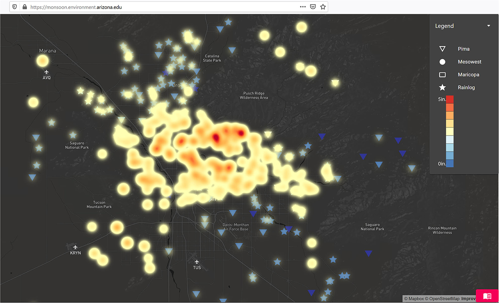
Figure 8. Tucson Metropolitan Region Total Precipitation - Jul 23, 2020 - Example of Heat Map Function of Monsoon Viewer.

FIGURE 9

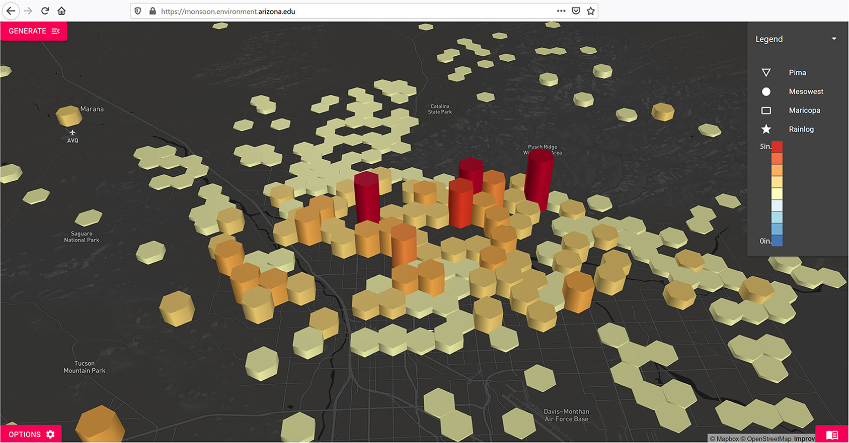
Figure 9. Tucson Metropolitan Region Total Precipitation - Jul 23, 2020 - Example of Hex Grid (3D) Function of Monsoon Viewer.

In late August 2020, a small precipitation event popped up in the afternoon. Most of the city recorded zero precipitation, but a small but intense storm was observed on the western edge of Tucson. A small number of stations recorded over 0.5″ of precipitation (Figure 10), but the storm was very limited in its extent. The monsoon viewer also includes recent MRMS data (within the last 7 days) to display the radar derived (gauge corrected) estimate of precipitation. For more widespread events, this offers an opportunity for ad hoc comparisons of point/station vs. gridded estimates of precipitation, but for the purposes of the viewer, it helps demonstrate instances when precipitation events are only captured in the station data. Figure 10 also includes the MRMS estimates as an overlay. Only one cell in the metropolitan area had an estimate over 0.00″.

FIGURE 10

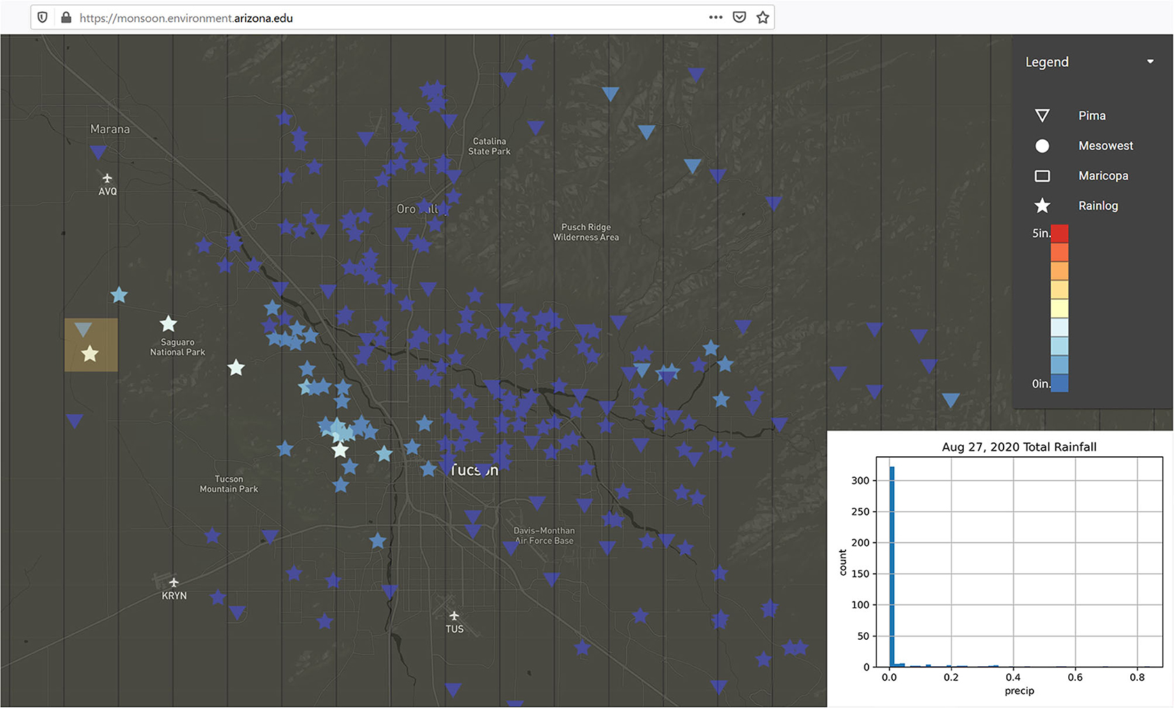
Figure 10. Tucson Metropolitan Region Total Precipitation - Aug 27, 2020 - Isolated Storm Event with Limited Data Coverage.

The inclusion of the MRMS data is also useful for a regional perspective, especially in locations where few if any weather stations are located. On August 30, daily forecasts indicated potential widespread and intense storm activity for the Tucson Metropolitan Area. These events did build and develop, but not quite as far east as some of the forecasts had initially suggested. Figure 11 shows the relatively limited precipitation that was recorded in the Tucson area, while the much more intense storm activity to the south and west is captured by the MRMS precipitation estimates. There are few stations located in this rural area, so the combination of station data in more densely covered areas in conjunction with the coarser estimates from MRMS, helps fill in information about where precipitation did (and did not) fall.

FIGURE 11

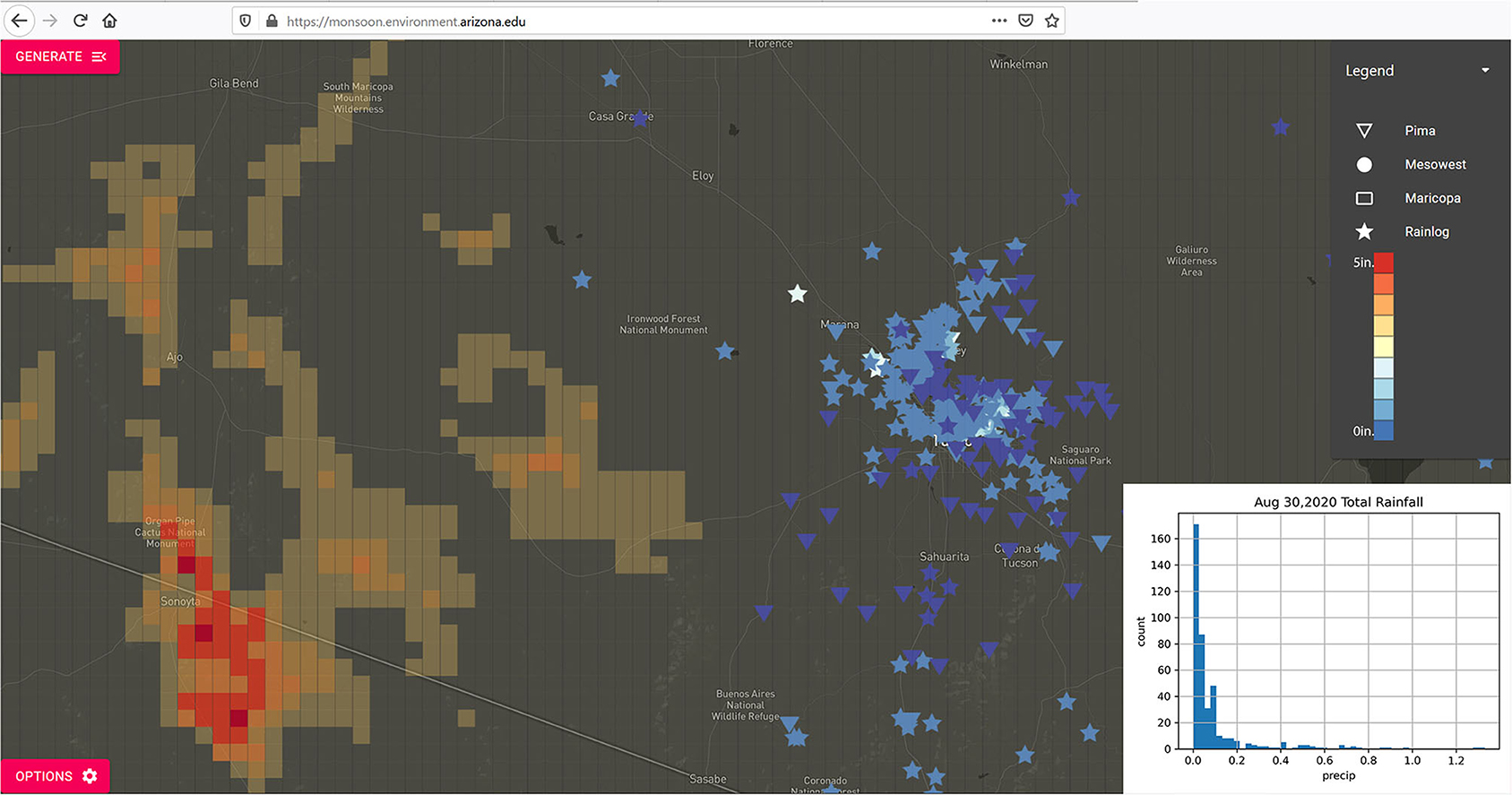
Figure 11. Pima County Region Total Precipitation - Aug 30, 2020 - Isolated Precipitation in Tucson Metro Area with Limited Data Coverage but with Heavy Precipitation in MRMS estimates in Western Pima County.

Inter-annual Comparisons

In addition to daily or event-based precipitation visualizations, the database (and particularly the Pima Flood Control District data, some of which goes back to the mid-1980's) also allows for some provisional comparison across years. This inter-annual comparison blunts some of the daily spatial variability, but these data summaries speak to what is sometimes referred to as the character or flavor of a given monsoon year.

A few of the most recent years are a helpful comparison to illustrate this use of these data. 2017 was widely regarded as a good year for the monsoon in Tucson. The Airport total was 8.57″, well above its long-term average of ~6.1″. Across the region stations also recorded precipitation at or above the airport's long-term average (Figure 12, top). Looking at the seasonal progression of events, these impressive totals were mostly the result of a pulse of very active monsoon precipitation in mid-to-late July, with one large event in August (Figure 12, bottom). 2018 by comparison, had both an early start with tropical storm Bud bringing precipitation to the region on June 15–16, a run of lighter but more regular monsoon activity for much of July and August, and then was capped with another tropical storm incursion in mid-September (Figure 13). Even though the airport recorded just over 7″ of rain in 2018 and had regular activity, it lacked the run of intense activity as was seen in 2017. Ongoing research within CLIMAS is using the monsoon viewer database to explore these spatial and temporal patterns in small scale monsoon precipitation events, and their connection to patterns and drivers of regional monsoon activity.

FIGURE 12

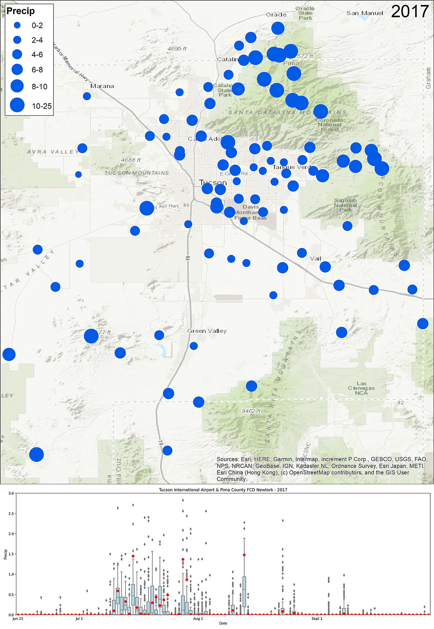
Figure 12. Map of Tucson Metropolitan Region 2017 Monsoon Total Precipitation - (Jun 15 - Sept 30) (map, top) and Range of Daily Precipitation (Jun 15 - Sept 30) compared to Tucson International Airport (boxplot, bottom).

FIGURE 13

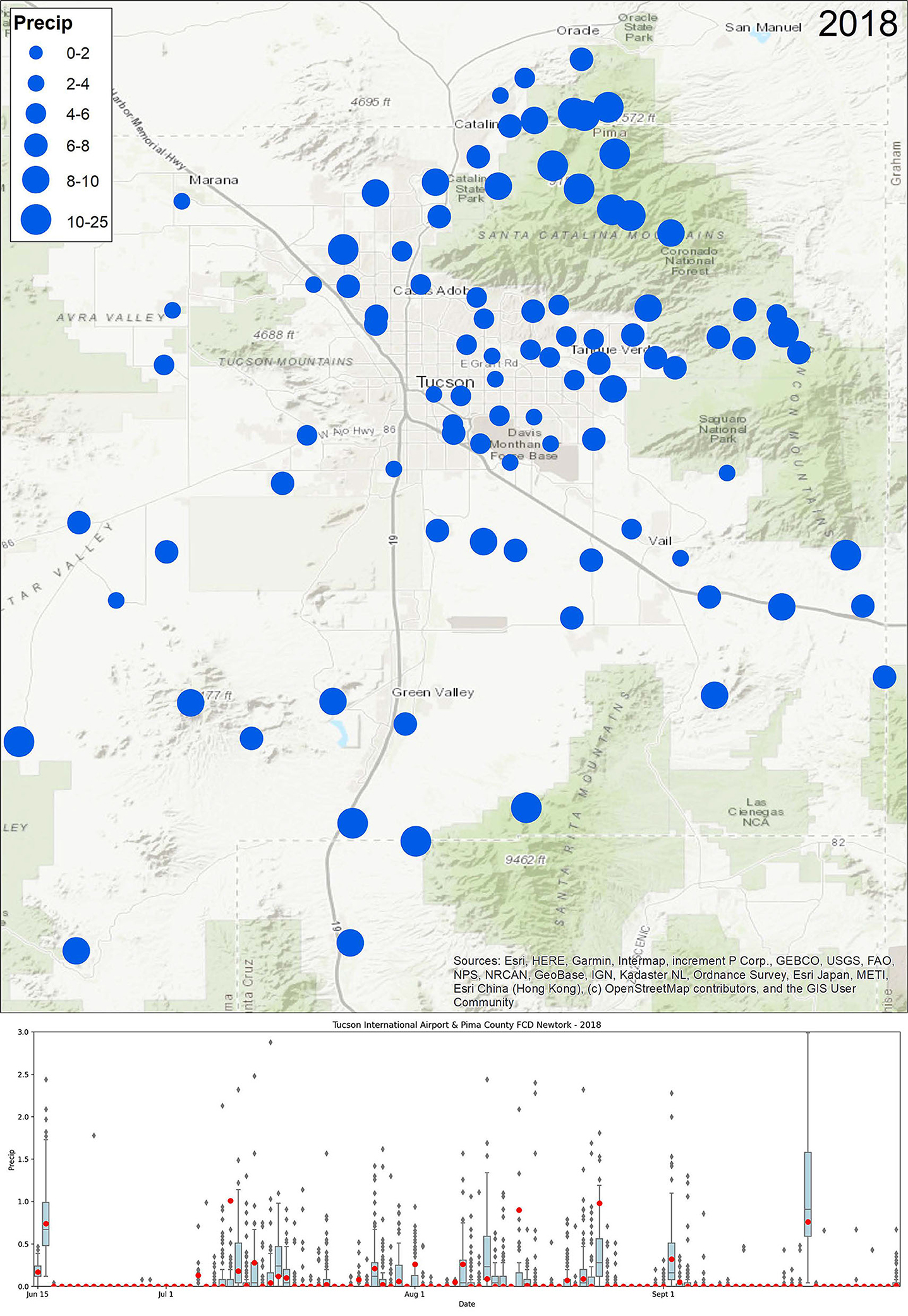
Figure 13. Map of Tucson Metropolitan Region 2018 Monsoon Total Precipitation - (Jun 15 - Sept 30) (map, top) and Range of Daily Precipitation (Jun 15 - Sept 30) compared to Tucson International Airport (boxplot, bottom).

Looking across multiple years of data, the percent of stations recording precipitation also helps fill in our understanding of how widespread monsoon activity was in the Tucson Metropolitan Region (Figure 14). This analysis is preliminary, and in conjunction with the spatial/temporal information mentioned above, is part of our larger and ongoing effort to use this database/viewer to illustrate regional precipitation variability. Our goal is to analyze and communicate not just how much precipitation fell at a given location, but how widespread these events were, and what this means for various applications that would benefit from granular spatial estimates (or longitudinal temporal characterizations) of monsoon precipitation.

FIGURE 14

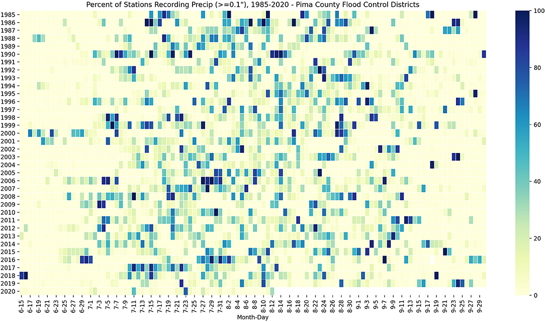
Figure 14. Daily Percent of Stations Recording Precipitation over 0.1″ during the monsoon (Jun 15 - Sept 30), 1985–2020.

Discussion

Despite a standardized seasonal definition that outlines the temporal boundaries of the monsoon across the Southwest, monsoon variability is challenging to accurately characterize at fine scales on the order of cities to neighborhoods. The monsoon viewer presented above characterizes monsoon precipitation variability in the U.S. Southwest, at scales that are not possible with single station metrics, and with a density of data that is not available in gridded datasets. Our initial goal for this platform was an improved characterization of fine-grained monsoon variability, informed by gaps and priorities of local stakeholders interested in updated and increasingly granular data about monsoon variability. We opportunistically focused on metropolitan regions with these larger networks of observations, and where there are known priorities for research applications or decision support. Our project analyzes the patterns we observe in the data and what it means for ongoing or potential research applications. Our project is also focused on the need for data curation and the role that computer science plays in helping integrate and visualize diverse and sometimes messy data cannot be underestimated.

This focus on metropolitan regions highlights a limitation of this approach, given dense sensor networks are typically only found in metropolitan regions such as Tucson (or Phoenix, Flagstaff, Albuquerque, El Paso, etc.), where there are sufficient sensors to offer additional granular information about precipitation variability. The inclusion of citizen science networks increases station density, but does little to significantly expand the extent of the networks, as many of these observers are also found in metropolitan regions. We added MRMS data to check the correspondence between point based (station) and gridded (radar derived) estimates of precipitation and to fill in gaps where few stations were found. A systematic comparison between these sources (see Westcott et al., 2008 for an example) is beyond the scope of this paper, but is part of a larger research project we have underway using these data. Despite the limited spatial extent of these data, these dense networks of observation can contribute to an improved understanding of fine-grained monsoon variability, identifying any coherent patterns that may exist at a regional, municipal, or even local neighborhood scale. This reflects emergent interest in targeted and fine scale analysis of weather and climate impacts, especially in urban and metropolitan contexts, as well as the decision making contexts that could be informed by these data and information (see Baklanov et al., 2018).

There are a number of contexts where these data could inform ongoing or future applied research, preparedness and emergency response activities, or long term planning and recovery efforts. What follows is a brief overview of collaborative applications either planned or underway.

An initial collaborator on this project was the National Weather Service office in Tucson, which indicated interest in a “monsoon event viewer” that stitched together station based precipitation data with the radar derived gridded estimates of precipitation from MRMS. Our ongoing work is assessing the correspondence between precipitation estimates in established sensor networks (e.g., Mesowest, RCC-ACIS), opportunistic sensor networks (e.g., flood control districts), citizen science observations (CoCoRaHS and Rainlog), and gridded data (including PRISM and MRMS estimates of daily and seasonal precipitation). Our goal is not to assess the accuracy of these data, but to see how well they correspond and if there is any indication as to best practices for assimilating multiple sources, types and scales of data.

From our participation in Pima County Hazard Mitigation workshops, we were aware of flood response and emergency management applications using these data. Given the potential for accumulated flood risk following a series of days in a row or a few days apart, the viewer and the fine-grained spatial and daily temporal data it presents could be used to assess regions that are likely to experience serious flooding were an additional storm to occur. This could be linked to the information about the saturation of soils, water already flowing in washes, or as is the case with the 2020 Bighorn Fire, post-fire flooding on wildfire scars. Participants at the workshop also identified cleanup and recovery efforts as another application, given the impact that floodwater can have in spreading sand and soil across roadways after flood events. A more precise estimate of precipitation location in conjunction with flow and wash data, could identify hotspots for cleanup and recovery following localized intense storm events.

The extreme spatial variability of the monsoon is also a challenge for irrigation control and water harvesting. An application could be useful to inform irrigation control and management after a series of storm events, rendering additional irrigation unnecessary. A map of spatial variability in the monsoon could identify regions where water harvesting tanks were likely to have filled given the location and intensity of precipitation. Notices to homeowners could be provided, especially if additional precipitation was in the forecast, with appropriate caveats about monsoon variability.

Finally, the USA National Phenology Network produces short-term forecasts of green-up in buffelgrass, an invasive grass that creates substantial fire risk to native desert plant and animal communities in the Southwestern US (https://usanpn.org/data/forecasts/Buffelgrass). The buffelgrass Pheno Forecast is based on known precipitation thresholds for triggering green-up to a level where management actions are most effective. These maps are updated daily using PRISM 4 km daily precipitation and predict green-up 1–2 weeks in the future, primarily during the summer monsoon period. Preliminary results indicate that the 4 km precipitation estimates provided by the PRISM dataset are often too coarse to detect sub-grid scale precipitation events that may trigger the green-up of local buffelgrass populations. The CLIMAS team is working with the NPN to utilize the monsoon viewer API to provide higher resolution precipitation data across the Tucson metropolitan region. These data will be used in conjunction with the PRISM precipitation grids to help provide sub-grid scale precipitation data points to help trigger and interpret bufflegrass green up forecasts.

On Collaboration Between Computer/Natural/Social Science

Climate services development and climate adaptation and impacts research has done well to encourage interdisciplinary approaches that embrace collaborative processes (Meadow et al., 2015; Owen et al., 2019) or which consider the type of climate services and platform for their use (Visscher et al., 2020). This collaborative focus builds on the foundation of well-articulated strategies regarding the role that data management and computer science applications could play in collecting, visualizing, and disseminating weather data (National Research Council, 2003). This foundation has been extended via emphasis on the global framework for climate services (GFCS) and associated frameworks for connecting data to users (Hewitt et al., 2012; Giuliani et al., 2017), or by tracing the value chain of climate data through data discovery, data integration, and the analysis, products and services that extend from this chain (Giuliani et al., 2017). Other work has emphasized design and interface issues, highlighting the need to focus user experience and interface (Christel et al., 2018).

The monsoon event viewer and API highlight the value and necessity of integrating computer science expertise into forward thinking climate services development. This provided a mechanism to aggregate and organize data, as well as a means to develop interactive design elements, with considerations of user experience and interface. Our initial use of dense network data demonstrated the utility of integrating information from multiple sources, but it also quickly revealed that our preliminary methods and approaches were not designed, much less capable, of scaling to anything that would resemble an operational product. We also learned it was important to integrate computer science and application development expertise into the core project team, to lead the database development process, and give guidance and input on visualization options and best practices. Put simply, this was more than tacking data science and aggregation onto existing climate services and highlighted the value of building and cultivating this collaboration early in the process. Regular meetings that brought together this interdisciplinary team were essential to discuss the database framework, design ideas for the viewer, and opportunities for additional data analysis. This process also identified technical challenges in managing the data, or issues which might affect visualization strategies. This ongoing dialogue allowed the team to identify priorities for version 1.0 of the visualizer, and to create a punch list of updates and fixes for subsequent versions. The project collaboration was also an opportunity for student training and experiential learning, providing a real-world application to test out and deploy innovative data aggregation, management, and visualization techniques from their studies. Faculty researchers working on the project also learned from this process, which helped them better understand the technological limitations of the various platforms, and how to integrate research questions into a feasible data aggregation and visualization framework. They also learned how to work with application/platform developers to revise the data visualizer, and to improve accessibility in the data/API. They also discussed existing and planned collaborations using these data and the API, to help refine the database and API development based on the needs of current or future stakeholder partners. These meetings and discussions drove the iterative development of the final platform and were a key part of our collective identification of version 1.0 of the viewer, which sits at the intersection of useful and technologically possible. Ongoing work continues to expand on both fronts.

This project also demonstrates the potential for external collaboration. We designed the visualizer and API with some known priorities in mind, as well as some presumed end-users who might be interested. We wanted the visualizer and API to be responsive to end-user priorities and useful based on expressed needs or gaps, but we also wanted to design a standalone platform that would allow for as-yet unknown end users to explore their own ideas for data visualization and data access. As such, we included the ability to download CSV files of the data, as well as an API for automated or systematic use of the data outside of the visualizer. These are still in beta with a soft launch of the monsoon viewer in August of 2020. One of our goals was to make a platform that would make these data widely accessible in a curated format for those that wanted a visualized overview. We also provide the raw data format via CSV download and the API for those that wanted to access the data and conduct the analyses themselves.

Data Availability Statement

Publicly available datasets were analyzed in this study. This data can be found here: monsoon.environment.arizona.edu.

Author Contributions

BM designed the study and led the research project activities. RG led the technological development team. BM and MC provided input on the network specifications and data attributes, and on the development of the monsoon visualizer platform. RG, BD, and MH developed the data aggregation, storage, and visualization platforms. BM, RG, BD, MH, and MC contributed to the final manuscript. All authors contributed to the article and approved the submitted version.

Funding

This work was supported in part by the University of Arizona's office of Research Discover and Innovation (now the office of Research, Innovation, and Impact - RII), and Climate Assessment for the Southwest (CLIMAS), which is part of the National Oceanic and Atmospheric Administration (NOAA) Regional Integrated Sciences and Assessments (RISA) program (Award Number: NA17OAR4310288).

Conflict of Interest

The authors declare that the research was conducted in the absence of any commercial or financial relationships that could be construed as a potential conflict of interest.

Acknowledgments

Special thanks to Zack Guido and Will Holmgren for their feedback and input. Additional thanks to careful and thoughtful comments provided by peer reviewers.

Supplementary Material

The Supplementary Material for this article can be found online at: https://www.frontiersin.org/articles/10.3389/fclim.2021.602573/full#supplementary-material

References

Adams, D. K., and Comrie, A. C. (1997). The North American monsoon. Bull. Amer. Meteor. Soc. 78, 2197–2213. doi: 10.1175/1520-0477(1997)078<2197:TNAM>2.0.CO;2

CrossRef Full Text | Google Scholar

Baklanov, A., Grimmond, C. S. B., Carlson, D., Terblanche, D., Tang, X., Bouchet, V., et al. (2018). From urban meteorology, climate and environment research to integrated city services. Urban Clim. 23, 330–341. doi: 10.1016/j.uclim.2017.05.004

CrossRef Full Text | Google Scholar

Christel, I., Hemment, D., Bojovic, D., Cucchietti, F., Calvo, L., Stefaner, M., et al. (2018). Introducing design in the development of effective climate services. Clim. Services 9, 111–121. doi: 10.1016/j.cliser.2017.06.002

CrossRef Full Text | Google Scholar

Crimmins, M. A. (2006). Arizona and the North American Monsoon System. University of Arizona Cooperative Extension, AZ1417.

Google Scholar

Crimmins, M. A., McMahan, B., Holmgren, W. F., and Woodard, G. (2021). Tracking precipitation patterns across a western U.S. metropolitan area using volunteer observers: RainLog.Org. Int. J. Climatol. doi: 10.1002/joc.7067. [Epub ahead of print].

CrossRef Full Text | Google Scholar

Demaria, E. M. C., Hazenberg, P., Scott, R. L., Meles, M. B., Nichols, M., and Goodrich, D. (2019). Intensification of the North American monsoon rainfall as observed from a long-term high-density gauge network. Geophys. Res. Lett. 46, 6839–6847. doi: 10.1029/2019GL082461

CrossRef Full Text | Google Scholar

Douglas, M. W., Maddox, R. A., Howard, K., and Reyes, S. (1993). The Mexican monsoon. J. Clim. 6, 1665–1667. doi: 10.1175/1520-0442(1993)006<1665:TMM>2.0.CO;2

CrossRef Full Text | Google Scholar

Ellis, A. W., Saffell, E. M., and Hawkins, T. W. (2004). A method for defining monsoon onset and demise in the southwestern USA. Int. J. Climatol. 24, 247–265. doi: 10.1002/joc.996

CrossRef Full Text | Google Scholar

Englehart, P. J., and Douglas, A. V. (2006). Defining intraseasonal rainfall variability within the North American monsoon. J. Clim. 19, 4243–4253. doi: 10.1175/JCLI3852.1

CrossRef Full Text | Google Scholar

Garcia, M., Peters-Lidard, C. D., and Goodrich, D. C. (2008). Spatial interpolation of precipitation in a dense gauge network for monsoon storm events in the southwestern United States. Water Resour. Res. 44, 1–18. doi: 10.1029/2006WR005788

CrossRef Full Text | Google Scholar

Giuliani, G., Nativi, S., Obregon, A., Beniston, M., and Lehmann, A. (2017). Spatially enabling the global framework for climate services: reviewing geospatial solutions to efficiently share and integrate climate data and information. Clim. Services 8, 44–58. doi: 10.1016/j.cliser.2017.08.003

CrossRef Full Text | Google Scholar

Goap, A., Sharma, D., Shukla, A. K., and Krishna, C. R. (2018). An IoT based smart irrigation management system using machine learning and open source technologies. Comput. Electron. Agric. 155, 41–49. doi: 10.1016/j.compag.2018.09.040

CrossRef Full Text | Google Scholar

Hewitt, C., Mason, S., and Walland, D. (2012). The global framework for climate services. Nat. Clim. Chang. 2, 831–832. doi: 10.1038/nclimate1745

CrossRef Full Text | Google Scholar

Higgins, R. W., Yao, Y., and Wang, X. L. (1997). Influence of the North American monsoon system on the US summer precipitation regime. J. Clim. 10, 2600–2622. doi: 10.1175/1520-0442(1997)010<;2600:IOTNAM>;2.0.CO;2

CrossRef Full Text | Google Scholar

Lemos, M. C., Kirchhoff, C. J., Kalafatis, S. E., Scavia, D., and Rood, R. B. (2014). Moving climate information off the shelf: boundary chains and the role of RISAs as adaptive organizations. Weather Clim. Soc. 6, 273–285. doi: 10.1175/WCAS-D-13-00044.1

CrossRef Full Text | Google Scholar

Maddox, R. A., McCollum, D., and Howard, K. (1995). Large-scale patterns associated with severe summertime thunderstorms over Central Arizona. Weather Forecast. 10, 763–778. doi: 10.1175/1520-0434(1995)010<;0763:LSPAWS>;2.0.CO;2

CrossRef Full Text | Google Scholar

Mahmood, R., Boyles, R., Brinson, K., Fiebrich, C., Foster, S., Hubbard, K., et al. (2017). Mesonets: mesoscale weather and climate observations for the United States. Bull. Am. Meteorol. Soc. 98, 1349–1361. doi: 10.1175/BAMS-D-15-00258.1

CrossRef Full Text | Google Scholar

Meadow, A. M., Ferguson, D. B., Guido, Z., Horangic, A., Owen, G., and Wall, T. (2015). Moving toward the deliberate coproduction of climate science knowledge. Weather Clim. Soc. 7, 179–191. doi: 10.1175/WCAS-D-14-00050.1

CrossRef Full Text | Google Scholar

Mullen, S. L., Schmitz, J. T., and Rennó, N. O. (1998). Intraseasonal variability of the summer monsoon over southeast Arizona. Monthly Weather Rev. 126, 3016–3035. doi: 10.1175/1520-0442(2002)015<2477:IVAWWM>2.0.CO;2

CrossRef Full Text | Google Scholar

National Research Council (2003). Fair Weather: Effective Partnership in Weather and Climate Services. Washington, DC: National Academies Press.

Google Scholar

NWS El Paso (2020). Available online at: https://twitter.com/NWSElPaso/status/1282536133885231104 (accessed July 12, 2020).

Owen, G., Ferguson, D. B., and McMahan, B. (2019). Contextualizing climate science: applying social learning systems theory to knowledge production, climate services, and use-inspired research. Clim. Change 157, 151–170. doi: 10.1007/s10584-019-02466-x

CrossRef Full Text | Google Scholar

Shoemaker, C. J. T., and Davis (2008). Hazardous Weather Climatology for Arizona. NOAA Technical Memorandum, NWS-WR 282, 47. Available online at: https://www.wrh.noaa.gov/images/twc/monsoon/TM-282.pdf (accessed August 15, 2020).

Google Scholar

Visscher, K., Stegmaier, P., Damm, A., Hamaker-Taylor, R., Harjanne, A., and Giordano, R. (2020). Matching supply and demand: a typology of climate services. Clim. Services 17:100136. doi: 10.1016/j.cliser.2019.100136

CrossRef Full Text | Google Scholar

Wallace, C. S., Walker, J. J., Skirvin, S. M., Patrick-Birdwell, C., Weltzin, J. F., and Raichle, H. (2016). Mapping presence and predicting phenological status of invasive buffelgrass in southern Arizona using MODIS, climate and citizen science observation data. Rem. Sens. 8:524. doi: 10.3390/rs8070524

CrossRef Full Text | Google Scholar

Westcott, N. E., Knapp, H. V., and Hilberg, S. D. (2008). Comparison of gage and multi-sensor precipitation estimates over a range of spatial and temporal scales in the Midwestern United States. J. Hydrol. 351, 1–12. doi: 10.1016/j.jhydrol.2007.10.057

CrossRef Full Text | Google Scholar

Zanchetta, A. D., and Coulibaly, P. (2020). Recent advances in real-time pluvial flash flood forecasting. Water 12:570. doi: 10.3390/w12020570

CrossRef Full Text | Google Scholar

Appendix

Referenced Technologies

Deck.gl docs – https://deck.gl/docs

React docs – https://reactjs.org/docs/getting-started.html

Express docs – https://expressjs.com/en/4x/api.html

Babel – https://babeljs.io/docs/en/

ES6 – https://www.ecma-international.org/ecma-262/7.0/

In Depth DOM – https://developer.mozilla.org/en-US/docs/Web/API/Document_Object_Model/Introduction

AWS Lambda – https://docs.aws.amazon.com/lambda/latest/dg/welcome.html

AWS S3 Hosting – https://docs.aws.amazon.com/AmazonS3/latest/dev/WebsiteHosting.html

AWS RDS – https://docs.aws.amazon.com/AmazonRDS/latest/UserGuide/Welcome.html

AWS EC2 Linux – https://docs.aws.amazon.com/AWSEC2/latest/UserGuide/concepts.html

GRIB2 – https://confluence.ecmwf.int/display/CKB/What+are+GRIB+files

MRMS – https://www.nssl.noaa.gov/projects/mrms/.

General Technical Overview/Appendix

There are several technologies required to gather, store, process, and present the data. Here you will find commonly referred to terms and services along with a short description of the functions they perform and links to documentation.

• Lambda

◦ Serverless/headless infrastructure used to execute scripts

◦ Run code without provisioning or managing servers or server instances.

◦ https://docs.aws.amazon.com/lambda/latest/dg/welcome.html

• EC2

◦ An EC2 Instance is a cloud computing solution allowing us to run various backend related tasks on a virtual machine

▪ This is equivalent to on premise server infrastructure without the cost of new infrastructure or physical systems administration needs.

◦ https://docs.aws.amazon.com/AWSEC2/latest/UserGuide/concepts.html

◦ AWS EC2 Instance T3a.Large

▪ Memory: 8GB

▪ vCPU: 2

▪ Storage: 30GB

▪ OS: Red Hat Enterprise Linux release 8.2 Ootpa

• RDS

◦ Cloud based relational database service with the ability to be hosted on scalable infrastructure that can be optimized for memory or read/write performance.

◦ Multiple database engines can be utilized such as Amazon Aurora, PostgreSQL, MariaDB, MySQL, Oracle, and Microsoft SQL Server.

▪ This project uses MariaDB

◦ https://docs.aws.amazon.com/AmazonRDS/latest/UserGuide/Welcome.html

• S3

◦ Scalable cloud-based object storage

◦ https://docs.aws.amazon.com/AmazonS3/latest/dev/WebsiteHosting.html

• React

◦ Framework for building user interfaces built on JavaScript

◦ https://reactjs.org/docs/getting-started.html

• Node.js

◦ A runtime environment for running JavaScript server-side built on Chrome's V8 JavaScript engine.

◦ https://nodejs.org/docs/latest-v12.x/api/

• Express

◦ A framework for building backend web applications in Node.js

◦ https://expressjs.com/en/4x/api.html

• Deck.gl

◦ A Web-GL JavaScript framework used for data visualization.

◦ https://deck.gl/docs

• Python

◦ A high-level programming language

◦ https://docs.python.org/3/.