Intuitively visualizing spatial data from biogeographic assessments: A 3-dimensional case study on remotely sensing historic shipwrecks and associated marine life

Introduction

Biogeographic assessments aim to quantify spatial and temporal relationships between organisms and their habitats to inform spatial planning decisions (Caldow et al., 2015). Complex spatial data streams resulting from biogeographic assessments, however, are challenging to communicate and translate into accessible formats that can inform resource management decisions and foster stakeholder engagement (Caldow et al., 2015). This challenge is especially pronounced in marine ecosystems, largely stemming from rapid technological innovations that enable scientists to more quickly and efficiently collect larger and more complex data at fine resolution and over expanded spatial and temporal scales (Porter et al., 2009). For example, active acoustics surveys, such as using echosounders to map seafloor habitats and detect biological organisms, including fish and plankton, can generate more than 2GB of data per minute during acquisition, and passive acoustic monitoring of marine soundscapes and soniferous organisms can accrete data at rates exceeding multiple GB of data per minute. Optical sensors, such as 4K and low-light video used to visually characterize ecosystems, can collect over several GB of imagery per minute, and photogrammetric [e.g., structure from motion (SfM)] imagery of seabed habitats and associated sessile organisms can breach 1 GB of imagery per m². Advances in marine robotics have allowed vehicles, such as autonomous underwater vehicles (Morris et al., 2014), autonomous surface vehicles (Ludvigsen et al., 2018), and uncrewed aerial vehicles (Ridge and Johnston, 2020), to be outfitted with acoustic and optical sensors further expand the reach and endurance to continuously collect data over broader spatial and temporal scales, amplifying the amount of data collected in marine ecosystems that require visualization and translation for biogeographic assessments.

Myriad approaches have been developed to more effectively convey highly quantitative, large, spatial data for resource managers and stakeholders by displaying these data within geographic information systems (GIS), often manifested through data or mapping portals and decision-support tools. These applications provide platforms that can integrate ecological, social, and economic information. For example, “Marine Cadstre” (https://www.marinecadastre.gov/), a government agency-supported data portal within the USA, provides spatial data to support resource management decisions, including offshore energy planning. As part of Marine Cadastre, a tool called OceanReports (https://www.marinecadastre.gov/oceanreports/) can output spatial characterizations and high-level spatial planning analyses of coastal ocean areas to further facilitate planning decisions. Formal decision-support tools, like the “Barbuda Blue Halo” (https://www.seasketch.org/), integrate multilevel survey information (e.g., habitat classifications, biological organism occurrence), allowing direct stakeholder interaction and exploration of the data. Decision-support tools come in many different forms to facilitate different aspects of spatial planning, as in the case of “Coexist” that merges simulation models and stakeholder consultations within an online framework aimed toward sustainably integrating aquaculture and fisheries in Europe (https://www.coexistproject.eu/). While these data portals and decision-support tools provide pathways for constituents to interact directly with and explore data, the tools do not always provide data in a visually intuitive, easy to understand manner. In fact, a recent review of decision-support tools for marine spatial planning concluded that future tools could benefit from expanded avenues for stakeholder engagement with data (Pinarbaşi et al., 2017), and another synthesis concluded that dramatic improvements are required when sharing data to the public (e.g., accessible, translated, effectively communicated) to foster a more transparent, integrated, and successful resource management process (Caldow et al., 2015).

Here, we present a case study detailing a novel approach for sharing complex, spatial data from biogeographic assessments in a three-dimensional (3D), interactive online format. The goal of our case study was to characterize and visualize cultural and ecological resources within and around the USA's first federally-designated National Marine Sanctuary, Monitor National Marine Sanctuary, to assess these resources. We also developed quantitative metrics for hypothesis-driven research on the ecological function of these resources (Paxton et al., 2019), but in this paper we focus on the 3D visualization of these complex data as a path toward disseminating and translating key spatial data to support resource management decisions and stakeholder engagement. Below we share our workflow and use it to illustrate how this visualization method can be applied to other coastal ecosystems, allowing seamless exploration of complex coastal spatial data stemming from biogeographic assessments.

Visualization approach

Overview

We simultaneously mapped shipwrecks and their associated fish on 19 historical shipwrecks off North Carolina, USA (Figure 1). The shipwrecks included the Civil War ironclad vessel, USS Monitor, which sank in 1862 and was later designated as the USA's first national marine sanctuary in 1975, as well as shipwrecks on the outer continental shelf of North Carolina (https://monitor.noaa.gov/). These surrounding shipwrecks include three from the World War I time period, two from the mid-1920's, and thirteen from World War II. The shipwrecks rest in waters ranging from 17 m (Ashkhabad) to 231 m deep (SS Bluefields). Each shipwreck was selected based on its historical significance, and some were also selected because they had not yet been assessed and data were required to support resource management decisions.

FIGURE 1

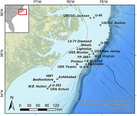
Figure 1. Locations of shipwrecks for which biogeographic assessments were conducted. Splitbeam echosounder and multibeam echosounder data from each shipwreck was displayed in three-dimensions within the “Living Shipwrecks 3D” visualization tool. Inset shows broader geographic context. Basemap credit: General Bathymetric Chart of the Oceans, NOAA National Centers for Environmental Information.

We surveyed each shipwreck using a suite of scientific echosounders, including a multibeam echosounder and splitbeam echosounders. We first collected high-resolution multibeam bathymetry imagery of each shipwreck. Using the resulting bathymetry, we then designed additional surveys to detect fish associated with the shipwrecks. These fish surveys were conducted using splitbeam echosounders and the watercolumn data from the multibeam echosounder and were designed in a grid survey pattern, with orthogonal along-shipwreck and across-shipwreck survey lines. Survey line spacing was determined based on the size of the shipwreck from the multibeam bathymetry imagery to enable adequate spatial coverage for fish detections.

Multibeam bathymetry

The multibeam echosounders (Reson 7125 and Kongsberg EM2040) collected multibeam bathymetry of each shipwreck at fine resolution (<1 m x 1 m cell size); the exact resolution was selected to provide optimal coverage based on the depth and anticipated shipwreck size. We corrected multibeam bathymetry data for changes in the speed of sound throughout the water column, tidal influence, static draft, latency, roll, pitch, yaw, and sensor offsets during post-acquisition processing (NOAA OCS, 2021). To display these data visually within a GIS framework, we imported the bathymetry elevation of each shipwreck as ground layers into a scene rendered within ESRI ArcGIS Pro version 2.4.0 (ESRI, 2020) and imported the corresponding geotiff of the bathymetry imagery into the ArcGIS Pro scene, as well.

Splitbeam echosounder

We detected fish associated with the shipwrecks using splitbeam echosounders. The splitbeam echosounders (Kongsberg Simrad EK60 with 7° beam angle) emitted sound pulses downwards into the water column at three frequencies and corresponding pulse lengths (38 kHz−0.256 μs, 120 kHz−0.128 μs, and 200 kHz−0.128 μs). Splitbeam ping emissions were triggered by multibeam pings to reduce interference among the echosounders. The hull-mounted transducers were calibrated for backscatter response using a tungsten carbide sphere (Demer et al., 2015). Following data acquisition, we processed raw echogram data within Echoview version 10.0 (Echoview Software Pty Ltd, 2020) to identify and characterize individual fish and schools of fish around the shipwrecks. We focused on the 120 kHz echosounder because data from this frequency were most commonly used by the authors in other studies for detecting fish across the varying shipwreck depths.

To detect individual fish, we applied a target detection and fish tracking algorithm that classifies sequential acoustic targets as discrete fish. Data for tracked individual fish were exported from Echoview with their corresponding latitude, longitude, depth, and target strength. These data were read into R version 3.5 (R Core Team, 2020) using a custom written script and exported as a shapefile. The shapefile was imported into ArcGIS Pro with the “Feature to 3D by Attribute” geoprocessing tool within the “3D Analyst” toolbox and displayed using at the identified geographic location and depth using a selected 3D symbology, where colored spheres sized proportionally to the mean target strength represent individual fish.

We applied a SHAPES school detection algorithm (Barange, 1994) to detect schools of fish and calculate geometric metrics associated with the schools, such as school thickness, school length, school perimeter, and school area. Data for fish schools were exported from Echoview with their corresponding centroid latitude, centroid longitude, centroid depth, and geometries (thickness, length, area, perimeter—all corrected for beam geometry). Similar to the workflow described for individual fish, we then read the exported data into R, exported the data from R as a shapefile, imported the shapefile into ArcGIS Pro to display the schools at the appropriate geographic coordinates and depth, and set 3D symbology where spheres represent fish schools. Sphere height was proportional to the corrected fish school thickness, whereas sphere width was proportional to the corrected fish school length. The presentation of schools in this way simplifies the shape of often irregular fish schools, but provides a standard presentation of relative size and extent across the seascape in the 3D visualization.

Multibeam watercolumn

The multibeam echosounder used to acquire multibeam bathymetry also collected watercolumn data. We used these watercolumn data to detect the across-ship path extent of fish schools associated with the shipwrecks. In comparison to the narrow (7°) beam width of the splitbeam echosounder, the broader (~130°) beam width of the multibeam echosounder permitted fish school detection of a larger area of the watercolumn around shipwrecks. Raw multibeam data were processed within Echoview to detect fish targets comprising a fish school. Data rates for the multibeam echosounder require significant computing and graphical resources. Therefore, for each shipwreck, we selected segments of transects that contained fish schools detected from the splitbeam echosounder data and then applied a multibeam target detection algorithm to subsets of ping transmissions in the data files, yielding a “cloud” of targets constituting the fish school. These identified multibeam fish targets representing the school were exported from Echoview by multibeam ping. For each ping, fish target values, including the target range, mean, major axis angle, and minor axis angle, were provided.

The multibeam fish target data were then read into R, where we performed geometric corrections accounting for ship position and motion to compute the position of each target in geographic space (latitude, longitude, depth). These processed data with a corresponding latitude, longitude, and depth for each target in the school were exported from R as a shapefile. The shapefile was imported into ArcGIS Pro, as per the splitbeam fish data described above, and set to the appropriate 3D symbology, where standard sized spheres represented fish targets—we did not vary sphere size by attribute because the multibeam system is uncalibrated and backscatter values are affected by numerous factors not limited to fish size and angular orientation relative to the acoustic beam. We also applied a convex hull to the multibeam fish targets within ArcPro, which allowed us to quantify the volume of the school, as well as the school width, thickness, and length. Ultimately, these schooling fish targets from the wider angle multibeam fan convey the broader spatial extent of the same fish schools that were originally detected and visualized in a narrower slice of the watercolumn using the splitbeam echosounder.

Data visualization

To visualize the multibeam bathymetry, splitbeam detected individual and schooling fish, and multibeam fish school extents, we next developed an online 3D tool using ArcGIS software products (Figure 2 and Supplementary Video S1). We exported each layer from the ArcGIS Pro scene (bathymetry, ground bathymetry, imagery, splitbeam individual fish, splitbeam fish schools, multibeam fish school extent) to the online NOAA Geoplatform using the “Share as Web Layer” tool. Once the layers were uploaded to the Geoplatform, we created a Web Scene to depict all layers in 3D using the following steps. First, we added a background ground layer to the Web Scene for ocean bathymetry that displays the broader geographic study area on a 3D ocean topography map (“TopoBathy 3D”) (ESRI, 2020). Second, we added the ground elevation layers for each shipwreck that display the bathymetry-derived shipwreck elevations in 3D. Third, we added the bathymetry-derived geotiff imagery of the shipwreck, which drapes over the ground elevation layer, providing a visual representation of the shipwreck. Fourth, we added the fish detection layers (splitbeam individual fish, splitbeam fish schools, multibeam fish school extent), which displayed in 3D around the ground elevation layers and accompanying geotiffs. We then imported the Web Scene into a Web Application. By pulling the Web Scene into a Web Application, we could customize the user interface by adding menus, navigation options, and styling to facilitate constituent exploration of and interaction with the multiple data streams.

FIGURE 2

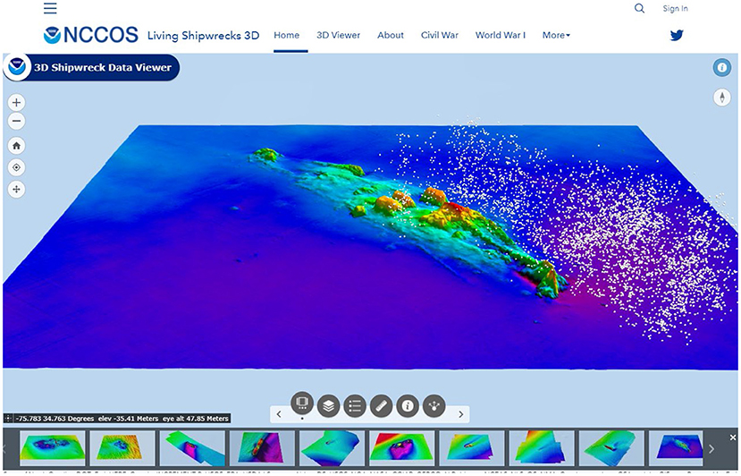
Figure 2. “Living Shipwrecks 3D” is an online interactive tool that displays habitat mapping data collected from acoustic surveys over shipwrecks, as well as photographs and videos. The tool combines bathymetry maps with maps of fish (white circles) detected with echosounders.

Once our data were compiled into the customized Web Application, we created an Arc Hub site. Arc Hub is an online ESRI software product that allows creation of customized web-page content using a GUI interface (ESRI, 2020). By using Arc Hub, we created a Hub Site called “Living Shipwrecks 3D” where we could combine visual media and story text with the data from the Web Scene and resulting Web Application (Figure 2 and Supplementary Video S1). The beauty of Arc Hub is that by building Hub Pages within the Hub Site, we can organize information into intuitive manners. For example, we created Hub Pages specific to shipwrecks from certain time periods to facilitate interaction with these data by stakeholders interested in history. The visual media that we added to the Hub Site included photographs and videos.

Conclusions

The “Living Shipwrecks 3D” visualization tool that we developed allows resource managers and stakeholders to directly access and engage with data in a way that best meets their needs. Resource managers can use the tool to understand the spatial extent and arrangement of shipwrecks and the spatial distributions of fish reliant upon the shipwrecks. For example, managers can measure the vertical height of shipwrecks from habitat mapping data and relate the vertical height to fish abundance and biomass. Information gained from interacting with remote sensing data can help inform resource management decisions on how to best ensure that shipwrecks remain special places within the seascape. Stakeholders, including those with an interest in ecology and history, can learn more about how shipwrecks function as habitat for marine life using the tool. For instance, recreational divers can use the tool to understand the layout of shipwrecks that they may visit for recreational dives.

We anticipate that additional interactive 3D data tools can be constructed using a similar workflow allowing seamless exploration of complex coastal spatial data used in biogeographic assessments. These tools can help overcome inherent challenges of visualizing and translating complex spatial datasets into formats that can be interpreted by diverse stakeholders and into actionable information to guide resource management decisions. Pursuits to develop similar visualization tools can help democratize data access.

Data availability statement

The datasets presented in this study can be found in online repositories. The names of the repository/repositories and accession number(s) can be found below: Data are archived and publicly available as: JT, AP, and EE. 2020. Living Shipwrecks 3D: Water column data in Southeast Atlantic, 2016-10-29 to 2018-08-21 (NCEI Accession 0215765). NOAA National Centers for Environmental Information Dataset. doi: 10.25921/y18j-8h61. The Living Shipwrecks 3D website is publicly available at https://3d-shipwreck-data-viewer-noaa.hub.arcgis.com/.

Author contributions

All authors conceptualized this research and reviewed and edited the manuscript. JT and TC acquired funding. EE processed multibeam bathymetry and splitbeam data. AP processed multibeam water-column data, created the 3D visualization tool, and drafted the manuscript. All authors contributed to the article and approved the submitted version.

Acknowledgments

We thank the NOAA National Centers for Coastal Ocean Science and Monitor National Marine Sanctuary for supporting this research. We thank the officers and crew of the NOAA ship Nancy Foster for supporting missions to collect data. AP was supported by CSS under NOAA/NCCOS Contract #EA113C17BA0062 during part of the study.

Conflict of interest

Author EE was employed by CSS-Inc. Author AP was employed by CSS-Inc. during part of the study.

The remaining authors declare that the research was conducted in the absence of any commercial or financial relationships that could be construed as a potential conflict of interest.

Publisher's note

All claims expressed in this article are solely those of the authors and do not necessarily represent those of their affiliated organizations, or those of the publisher, the editors and the reviewers. Any product that may be evaluated in this article, or claim that may be made by its manufacturer, is not guaranteed or endorsed by the publisher.

Author disclaimer

The views and conclusions contained in this document are those of the authors and should not be interpreted as representing the opinions or policies of the US Government, nor does mention of trade names or commercial products constitute endorsement or recommendation for use.

Supplementary material

The Supplementary Material for this article can be found online at: https://www.frontiersin.org/articles/10.3389/fclim.2022.1011194/full#supplementary-material

Supplementary Video S1. Tour of the “Living Shipwrecks 3D” online tool. The video tour of the tool showcases data associated with two shipwrecks: USS Tarpon and Proteus.

References

Barange, M. (1994). Acoustic identification, classification and structure of biological patchiness on the edge of the Agulhas Bank and its relation to frontal features. South Afr. J. Marine Sci. 14, 333–347. doi: 10.2989/025776194784286969

CrossRef Full Text | Google Scholar

Caldow, C., Monaco, M. E., Pittman, S. J., Kendall, M. S., Goedeke, T. L., Menza, C., et al. (2015). Biogeographic assessments: a framework for information synthesis in marine spatial planning. Marine Policy 51, 423–432. doi: 10.1016/j.marpol.2014.07.023

CrossRef Full Text | Google Scholar

Demer, D. A., Berger, L., Bernasconi, M., Bethke, E., Boswell, K., Chu, D., et al. (2015). Calibration of Acoustic Instruments. ICES Cooperative Research Report No. 326. p. 133. doi: 10.25607/OBP-185

CrossRef Full Text | Google Scholar

Echoview Software Pty Ltd (2020). Echoview Software. Hobart, Australia: Echoview Software Pty Ltd.

Google Scholar

ESRI (2020). ArcGIS Pro. Redlands, California, USA. Redlands, California, United States: Environmental Systems Research Institute. Environmental Systems Research Institute.

Ludvigsen, M., Berge, J., Geoffroy, M., Cohen, J. H., De La Torre, P. R., Nornes, S. M., et al. (2018). Use of an Autonomous Surface Vehicle reveals small-scale diel vertical migrations of zooplankton and susceptibility to light pollution under low solar irradiance. Sci. Adv. 4, eaap9887. doi: 10.1126/sciadv.aap9887

PubMed Abstract | CrossRef Full Text | Google Scholar

Morris, K. J., Bett, B. J., Durden, J. M., Huvenne, V. A. I., Milligan, R., Jones, D. O. B., et al. (2014). A new method for ecological surveying of the abyss using autonomous underwater vehicle photography. Limnol. Oceangraph. Method. 12, 795–809. doi: 10.4319/lom.2014.12.795

CrossRef Full Text | Google Scholar

NOAA OCS (2021). Hydrographic Survey Specifications and Deliverables. NOAA Office of Coast Survey, Hydrographic Surveys Division.

Paxton, A. B., Taylor, J. C., Peterson, C. H., Fegley, S. R., and Rosman, J. H. (2019). Consistent spatial patterns in multiple trophic levels occur around artificial habitats. Marine Ecol. Prog. Series 611, 189–202. doi: 10.3354/meps12865

CrossRef Full Text | Google Scholar

Pinarbaşi, K., Galparsoro, I., Borja, Á., Stelzenmüller, V., Ehler, C. N., and Gimpel, A. (2017). Decision support tools in marine spatial planning: present applications, gaps and future perspectives. Marine Policy 83, 83–91. doi: 10.1016/j.marpol.2017.05.031

CrossRef Full Text | Google Scholar

Porter, J. H., Nagy, E., Kratz, T. K., Hanson, P., Collins, S. L., Arzberger, P., et al. (2009). New eyes on the world: advanced sensors for ecology. BioScience 59, 385–397. doi: 10.1525/bio.2009.59.5.6

PubMed Abstract | CrossRef Full Text | Google Scholar

R Core Team (2020). R: A Language and Environment for Statistical Computing. Vienna, Austria: R Foundation for Statistical Computing.

Google Scholar

Ridge, J. T., and Johnston, D. W. (2020). Unoccupied aircraft systems (UAS) for marine ecosystem restoration. Front. Marine Sci. 7, 438. doi: 10.3389/fmars.2020.00438

CrossRef Full Text | Google Scholar