Deep learning for skillful long-lead ENSO forecasts

Patil, Kalpesh Ravindra; Doi, Takeshi; Jayanthi, Venkata Ratnam; Behera, Swadhin

doi:10.3389/fclim.2022.1058677

ORIGINAL RESEARCH article

Front. Clim., 04 January 2023
Sec. Predictions and Projections
Volume 4 - 2022 | https://doi.org/10.3389/fclim.2022.1058677

Deep learning for skillful long-lead ENSO forecasts

Kalpesh Ravindra Patil^*

Takeshi Doi

Venkata Ratnam Jayanthi

Swadhin Behera

Application Laboratory (APL), Research Institute for Value-Added-Information Generation (VAiG), Japan Agency for Marine-Earth Science and Technology (JAMSTEC), Yokohama, Japan

El Niño-Southern Oscillation (ENSO) is one of the fundamental drivers of the Earth's climate variability. Thus, its skillful prediction at least a few months to years ahead is of utmost importance to society. Using both dynamical and statistical methods, several studies reported skillful ENSO predictions at various lead times. Predictions with long lead times, on the other hand, remain difficult. In this study, we propose a convolutional neural network (CNN)-based statistical ENSO prediction system with heterogeneous CNN parameters for each season with a modified loss function to predict ENSO at least 18–24 months ahead. The developed prediction system indicates that the CNN model is highly skillful in predicting ENSO at long lead times of 18–24 months with high skills in predicting extreme ENSO events compared with the Scale Interaction Experiment-Frontier ver. 2 (SINTEX-F2) dynamical system and several other statistical prediction systems. The analysis indicates that the CNN model can overcome the spring barrier, a major hindrance to dynamical prediction systems, in predicting ENSO at long lead times. The improvement in the prediction skill can partly be attributed to the heterogeneous parameters of seasonal CNN models used in this study and also to the use of a modified loss function in the CNN model. In this study, we also attempted to identify various precursors to ENSO events using CNN heatmap analysis.

1. Introduction

The effects of El Niño-Southern Oscillation (ENSO) events on weather and climate, which have been linked to numerous climate calamities worldwide, have been extensively discussed and well-documented in the past (Ropelewski and Halpert, 1987; Trenberth et al., 1998; Alexander et al., 2002; Domeisen et al., 2019; Taschetto et al., 2020). The ability to forecast ENSO events and their associated climatic impacts well in advance of their onset is critical for the effective management of ENSO, which has been linked to numerous climate calamities worldwide.

El Niño-Southern Oscillation has been theorized to be predictable for at least 2 years in advance (Jin et al., 2008; Luo et al., 2008). However, the predictability at long lead times of up to 2 years and beyond is still challenging due to the unresolved teleconnection processes. The state-of-the-art dynamical models have shown success in ENSO forecasting of up to 1 year lead time (Luo et al., 2005, 2008; Jin et al., 2008; Barnston et al., 2017), but forecasts generated beyond that show moderate to poor forecasting skills, apparently due to the spring predictability barrier (Latif et al., 1994; Torrence and Webster, 1998; Luo et al., 2005, 2008; Lopez and Kirtman, 2014). Various statistical models were also developed for ENSO forecasting in the past, and some of them are seen to outperform the dynamical models with a sufficient difference at the 1-year lead time (Barnston et al., 1994; Tangang et al., 1997; Dijkstra et al., 2019; Ham et al., 2019, 2021a; Yan et al., 2020). But they show marginal improvements at the longer lead times. With recent advances in statistical methods, ENSO forecasting shows the possibility of skillful forecasts at 1.5- to 2-year-lead time and has succeeded in pushing the spring predictability barrier a few seasons further than the dynamical models (Ham et al., 2019; Hu et al., 2021; Mu et al., 2021; Zhou and Zhang, 2022).

The studies carried out so far using the convolutional neural network (CNN) model had some limitations in their setup to forecast ENSO at long lead times, such as the lack of updating the model parameters for each season and training them using a trivial loss function (Ham et al., 2019, 2021a; Geng and Wang, 2021; Hu et al., 2021; Mu et al., 2021). We attempt to address such limitations in this study and further improve the lead time of ENSO prediction. Moreover, ENSO shows strong physical linkages with the slowly evolving oceanic components in the tropical Pacific (Chen et al., 2004; Moon et al., 2007; Luo et al., 2008; Ramesh and Murtugudde, 2012; Ogata et al., 2013; Zhao et al., 2021), Indian Ocean (Behera et al., 2006; Izumo et al., 2010; Luo et al., 2010; Kug and Kang, 2006), Atlantic Ocean (Ham et al., 2013, 2021a; Chikamoto et al., 2020; Richter and Tokinaga, 2020), western hemisphere warm pool (Park et al., 2018), and North Pacific regions (Larson and Kirtman, 2014; Pegion and Selman, 2017; Tseng et al., 2017) at longer lead times. They can work as potential sources of the long lead predictability of ENSO.

Among various recent deep learning schemes, the CNN has shown significant success in the oceanic (de Silva et al., 2021; Huang et al., 2022; Jahanbakht et al., 2022; Patil and Iiyama, 2022) and climate applications (Reichstein et al., 2019; Baño-Medina et al., 2021; Liu et al., 2021; Cheng et al., 2022), including the ENSO forecasting (Ham et al., 2019, 2021b; Geng and Wang, 2021; Hu et al., 2021; Mu et al., 2021), due to its fine ability to correlate the intricate patterns within the spatio-temporal data with the target (Krizhevsky et al., 2012). Therefore, in the current study, we propose a forecasting scheme for ENSO at very long lead times (up to 3 years) based on CNN by additionally taking into account the varying parameters of CNN models for each season and training them with a customized loss function which considers extreme ENSO events separately. This is a kind of a novel attempt compared to previous studies of deep learning applied to climate predictions (Ham et al., 2019, 2021b; Geng and Wang, 2021; Hu et al., 2021; Liu et al., 2021; Mu et al., 2021; Feng et al., 2022). We train the CNN models using the past monthly global sea-surface temperature anomalies (SSTA) and vertically averaged subsurface ocean temperature anomaly (VATA) (averaged over 0–300 m depth, a proxy for heat content) fields. Model skills are compared with persistent forecasts, dynamical models, and previous deep-learning-based forecasts. In addition, we ran a heatmap analysis to confirm the significant oceanic regions that contribute to subsequent ENSO episodes.

2. Datasets

To provide robustness in the validation procedure, datasets from different sources were used in the calibration and validation process. For the calibration phase, SSTA data from Centennial In Situ Observation-Based Estimates (COBE) (Ishii et al., 2005) and VATA from Simple Ocean Data Assimilation (SODA) (Carton and Giese, 2008) were used; whereas, for the validation phase, SSTA from NOAA Optimum Interpolation SST v2 (OISSTv2) (Reynolds et al., 2007) and VATA from Global Ocean Data Assimilation System (GODAS) (Behringer and Xue, 2004) were used as predictors of the CNN.

In this study, we target the prediction of the Nino 3.4 index, a representative of ENSO events (Trenberth and Hoar, 1996), estimated by averaging the spatial SSTA over the Nino3.4 region [170°-120°W, 5°S−5°N]. The index is smoothed with a 3-month running mean during the calibration and validation phases to reduce the impact of high-frequency variations. The model calibration phase spans over 110 years, ranging from 1871 to 1980, using COBEv2 data, and that of the validation phase spans over 38 years, from 1984 to 2021, using OISSTv2 data. To provide robustness in the validation procedure, distinct datasets for the calibration and validation phases were used. Anomalies were calculated by removing the corresponding climatologies from 1981 to 2020 and re-gridded to a 5° × 5° spatial resolution. To achieve a 5° × 5° spatial resolution, datasets were re-gridded using bilinear interpolation from the source grid. Furthermore, standardization and normalization (−1 to +1 range) at each grid were performed to take into account the varying source of data and the limits of the transfer function, respectively.

3. Model and methods

We used CNN to accomplish multiyear ENSO forecasts using the past 3 monthly SSTA and VATA fields as predictors over the 0°-360°E, 55°S−60°N region. The lead time in forecasting is calculated from the center month of predictors to the center months of the target 3 monthly averaged Nino3.4 index. For example, the lead time between May–July (MJJ) 1996 predictors and Dec–Feb (DJF) 1997/98 target Nino3.4 index is 18 months.

The convolutional neural network was chosen above other deep learning approaches because of its capacity to handle spatiotemporal inputs and detect probable predictability sources from them (Krizhevsky et al., 2012). Even though several previous studies have also shown very promising results of using CNN toward prediction and analysis problems related to ocean and climate studies, including ENSO forecasting, we observe some important shortcomings in them.

In this study, we improved the proposed statistical scheme based on CNN in three aspects considering the limitations noted in the preceding studies of ENSO forecasting. These improvements include (a) separate CNN models for each season with varying internal parameters, (b) the loss function used for training the CNN models, which accounts for the extreme ENSO events, and (c) layers (average pooling, batch normalization) that followed convolutional layers.

3.1. Proposed CNN architecture

The proposed CNN consists of three convolutional layers that extract important spatial features from the predictors (i.e., SSTA and VATA). Each convolutional layer was followed by an average pooling layer to reduce the model parameters without losing the extracted features. After each average pooling layer, further layers were added to avoid over-fitting, which include dropout, regularization, and batch-normalization layers. Dropout layers ensure the filtering of unnecessary parts from the input, regularization layers ensure the penalization of the large-sized weights, whereas batch-normalization ensures further normalization of inputs after each convolutional process.

One block of the proposed CNN model consists of convolutional, average pooling, drop-out, regularization, and batch-normalization layers; three such blocks were used for each seasonal CNN. Furthermore, dense layers were added after three blocks to output an ENSO event which was compared against the observed ENSO event and based on the observed error, the parameters of CNN were optimized using a customized loss function. Figure 1 depicts briefly the architecture of the proposed CNN and Equation (1) elaborates on the feature extraction process. The training of the proposed CNN was done on JAMSTEC's Earth Simulator under Python 3.6 environment using Tensorflow 2.2.4 (Abadi et al., 2016) in the background and Keras 2.4.1 (Chollet, 2015) at the front end.

\begin{array}{l} N i n o 3 . 4 i n d e x_{t} = \\ \sum_{l = 1}^{L} (a v g P (\sum_{f = 1}^{M} \sum_{I N P_{t - l d}} σ (\sum_{i = 1}^{w \times h} (W_{i f l} R_{i l}) + b_{f l}))) & (1) \end{array}

where;

INP_t−ldglobal SSTA, VATA map of size (lat × lon), for the first convolutional layer,

feature maps for subsequent convolutional layers of size ((lat − h + 1)/2, (lon − w + 1)/2).

ld—lead time in months.

M–Number of convolutional filters with height (h), width (w).

R_il–region where Mfocuses on part of the complete input image INP_t−ld.

W_ifl–weight matrix of size “M,” shared over various regions of INP.

b_fl–bias vector of convolutional filters.

avg–Paverage pooling over region focused by “M'.

L–number of convolutional layers.

FIGURE 1

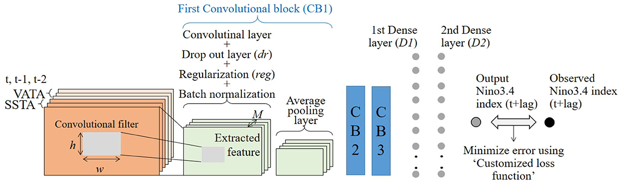
Figure 1. Architecture of the seasonally varying CNN models proposed for ENSO forecasts, trained using the past 3 monthly global spatial fields of SSTA and VATA. Various additional layers of dropout, regularization, and batch normalization are added after the convolution layer for avoiding overfitting. Training is performed using a customized loss function. Various internal CNN parameters are obtained using random search algorithms over 300 different trials.

3.2. Customized loss function to train the CNN

We propose a novel customized loss function for the training of proposed seasonal CNN, unlike the trivial one, i.e., mean square error as reported in numerous past studies of CNN. In this customized loss function, we calculate the mean square error between observed and forecasted ENSO events, and in addition to it, we add a penalty to this error if the observed ENSO event crosses one standard deviation for the respective season. Equation (2) further elaborates on the customized loss function used for optimizing the CNN parameters, in which the first part is the usual mean square error loss and the second part is additional loss added only for extreme ENSO events with a penalty.

\begin{array}{l} \begin{array}{l} C u s t o m i z e d l o s s f u n c t i o n = \\ \frac{1}{N} \sum^{​} {(O b s_{N 3 . 4} - P r e d_{N 3 . 4})}^{2} + \\ α^{*} \frac{1}{N} \sum^{​} {(O b s_{N 3 . 4_{_e x t}} - P r e d_{N 3 . 4})}^{2} \end{array} & (2) \end{array}

where, N—Total number of validation months (38 months),

Obs_N3.4–Observed Nino3.4 index,

Pred_N3.4–Forecasted Nino3.4 index,

α–penalty factor extreme events loss 0.5 to 1.75,

Obs_{N3.4_ext}–Extreme ENSO events separated using one standard deviation as a threshold for the respective season.

3.3. Seasonally varying internal CNN parameters

Due to its seasonal foot-printing mechanism, ENSO amplitude shows high seasonal variability, and each seasonal CNN has different parameters to account for such high variability. These parameters include initial weights of CNN, convolutional filter size, number of convolutional filters, drop out ratio, regularization penalty factor, customized loss function penalty factor, number of dense layers, number of neurons in each dense layer, epochs (number of training cycles), learning rates, and cross-validation period (testing of the trained parameters at the initial, middle, or end of the total calibration period). The limits of these various parameters are briefed in Supplementary Table S1. It is quite advantageous to vary these parameters to enhance forecasting ability (Bergstra and Bengio, 2012). Furthermore, each seasonal CNN was initialized with 300 trials of different combinations of these parameters. These 300 trials were ranked in decreasing order of performance using higher correlation skill and lower mean square error values 1–10, and the top ten members were retained as ensemble members.

3.4. Heatmaps

We analyzed the important regions contributing to skillful ENSO forecasts in CNN using heatmaps. These heatmaps are multiplications of an activation map from the first or third convolutional layer with gradients from the same layer. The heatmaps are extracted from the best ensemble member among the top ten. These heatmaps have been proposed by Selvaraju et al. (2020) and were further found useful for estimating the relative contribution of the predictors in a few recent past studies (Liu et al., 2021; Feng et al., 2022). Equation (3) elaborates on the estimation of activation maps for specific convolutional layers (Krizhevsky et al., 2012) and Equation (4) elaborates on the extraction of gradients from a specific layer (Selvaraju et al., 2020). The proposed GradCAM heatmaps are generated by multiplying Equations (3) and (4).

\begin{array}{l} A c t M a p = \sum_{f = 1}^{M} \sum_{I N P_{t - l d}} σ (\sum_{i = 1}^{w \times h} (W_{i f l} R_{i l}) + b_{f l}) & (3) \end{array}

\begin{array}{l} \frac{\partial L}{\partial X_{i}} = \sum_{m = 1}^{M} \frac{\partial L}{\partial O_{m}} \times \frac{\partial O_{m}}{\partial X_{i}} & (4) \end{array}

where;

L - Customized loss function, M - number of filters in last convolutional layer.

X_i - output of the current layer, i - number convolutional filters,

O_m - outputs from last layer (Pred_N3.4).

3.5. SINTEX-F2 dynamical prediction system

The dynamical seasonal prediction system is based on a fully coupled global ocean–atmosphere circulation model (CGCM) called SINTEX-F ver. 2 developed under the EU–Japan collaborative framework (Masson et al., 2012; Sasaki et al., 2013). This system adopts a relatively simple initialization scheme based only on the nudging of the SST data (Doi et al., 2016) and a three-dimensional variational ocean data assimilation (3DVAR) method by taking three-dimensional observed ocean temperature and salinity data into account (Doi et al., 2017). In consideration of the uncertainties of both initial conditions and model physics, the system had 12 members for the 24-month lead predictions initiated on the first day of each month from 1983 to 2015 (Doi et al., 2019). Although the previous version of the SINTEX-F is also skillful at predicting seasonal climate anomalies of up to a 2-year lead during specific ENSO years, the prediction skills of ENSO beyond a 1-year lead time are partly improved by the SINTEX-F2 (Behera et al., 2021).

4. Results

The ENSO forecasts generated from the proposed CNN models were validated for the ensemble mean over the ten best ensemble members from 1984 to 2021 against the Nino3.4 index calculated from the OISSTv2 dataset. Skill assessment of these ENSO forecasts was done using deterministic and probabilistic skill measures, namely correlation coefficient and relative operating characteristic curve (ROC), respectively.

4.1. Deterministic skills

4.1.1. Multi-year all season ENSO index correlation skill

Correlation coefficients (hereafter, correlation skills) are used to evaluate the model's deterministic skill score. Figure 2 shows the comparison of correlation skills for ENSO forecasts, namely seasonally varying-parameter CNN models, fixed-parameter CNN models, and reforecast output from the SINTEX-F2 dynamical model (hereafter SINTEX-F2) as a function of lead time ranging from 12 to 36 months. The correlation skill is compared for all season-forecasted ENSO indices obtained by combining the forecasted ENSO index from individual seasonal CNN models.

FIGURE 2

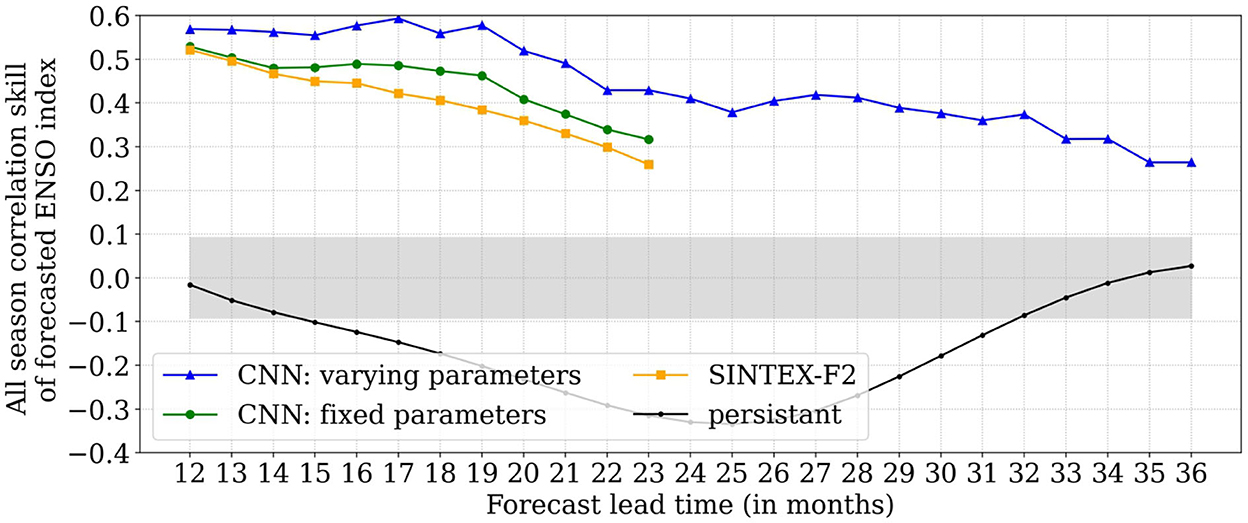
Figure 2. Multi-year CNN ensemble mean correlation skills as a function of lead time for all season forecasted ENSO index combined from each seasonal CNN model (blue) compared with fixed parameter CNN model (green), SINTEX-F2 (orange), and persistent predictions (black) (calculated from OISSTv2). Validation of CNN experiments is done using the observed ENSO index calculated from OISSTv2 data over 38 years from 1984 to 2021, whereas validation of SINTEX-F2 is done from the period 1984 to 2015 (32 years). Correlations outside light gray shading are statistically significant at a 95% level based on Student's 2-tailed t-test.

The all-season correlation skills of the forecasted ENSO index for seasonally varying parameter CNN models show higher values ranging from 0.57 to 0.40 for 12- to 23-month lead times, whereas the same for fixed parameter CNN and SINTEX-F2 are much lower, from 0.48 to 0.25 (Figure 2). The performance of the CNN with fixed parameters is similar to that reported in earlier studies by Ham et al. (2019, 2021b), Yan et al. (2020), Hu et al. (2021), Mu et al. (2021), and Geng and Wang (2021). Both the varying and fixed parameter CNN models outperform the SINTEX-F2 dynamical model over 12–23-month lead times. The performance of the CNN model is also better than the persistence (Figure 2).

Encouraged by the performance of the CNN model in predicting the ENSO index of up to the 24-month lead time, we extended the forecast seasonally varying CNN model predictions to even lead times of up to 3 years. As seen in Figure 2, the all-season forecasted ENSO index correlation skill is modest but is higher than 0.35 from 2 to 2.5 years of lead time; afterward, it drops to 0.25 at around 3 years of lead time. However, the CNN performs better than persistence, even for a lead time of 3 years (Figure 2).

4.1.2. Seasonal variation of correlation skill

Because ENSO has a seasonal phase-locking nature, it is likely to have a similar effect on the forecasting skills for individual seasons. Figure 3A shows seasonal variation in the ensemble mean correlation skills for the forecasted seasonal ENSO index from seasonally varying CNN models of over 12–23 months of lead times, validated against observed seasonal ENSO index calculated from the OISSTv2 dataset from 1984 to 2021. The correlation skill of seasonally varying CNN models is observed to be higher than 0.6 during most of the target seasons for 12–18 months of lead time, except for a few. SINTEX-F2 was observed better only during the winter and spring seasons but with poor correlations for other seasons relative to the CNN model. Moreover, high correlation skills of > 0.6 for the proposed CNN are continued till 21 months of lead time for the winter (DJF) season. The corresponding skill is below 0.4 after 18 months of lead time for SINTEX-F2 and other fixed parameter CNN models evaluated in this study as well as some previous studies, such as Ham et al. (2019), Hu et al. (2021), Mu et al. (2021), and Zhou and Zhang (2022).

FIGURE 3

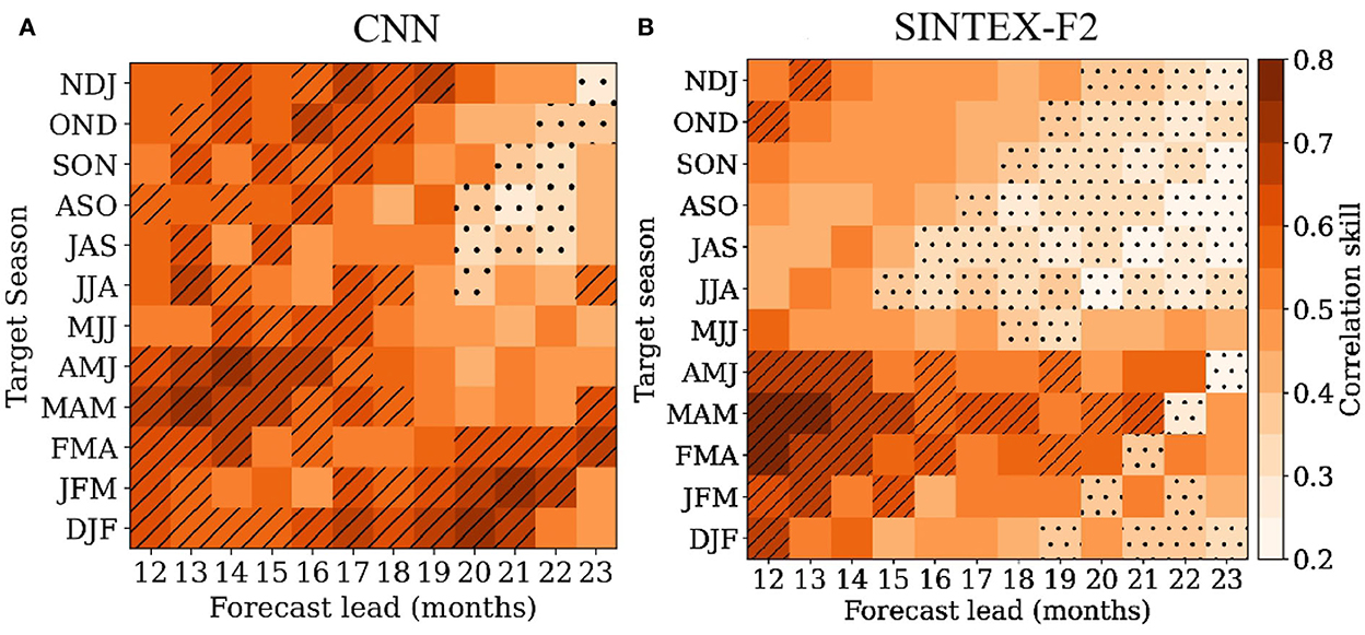
Figure 3. Ensemble mean correlation skills during each target season from seasonally varying CNN models (A) compared against SINTEX-F2 (B) through 12–23 months lead time. The validation period for the CNN experiment is 1984–2021 and SINTEX-F2 is 1985–2015. Hatching and dots represent the correlations >0.6 and <0.4, respectively. Correlations above 0.32 are statistically significant at a 95% level based on Student's 2-tailed t-test.

Furthermore, it is critical to comprehend the model prediction capabilities' behavior in relation to the spring predictability barrier. Because of ENSO's strong seasonal phase-locking nature, the forecast skills for the boreal spring season have rapidly declined, allegedly due to the least resilient ocean–atmosphere system during spring (Webster and Yang, 1992). Such a spring barrier has been seen for SINTEX-F2 (Figure 3B) and previous deep learning ENSO forecasting research (Ham et al., 2019; Hu et al., 2021; Mu et al., 2021; Zhou and Zhang, 2022), where prediction skills deteriorated during the spring season. However, this deterioration was noticed with greater severity around 14 months lead time and continued to be bad for both SINTEX-F2 (Figure 3B) and previous deep learning investigations. Interestingly, seasonally variable CNN models show comparable prediction abilities across all seasons (Figure 3A), with the first rapid reduction occurring at a somewhat late lead time, around 20 months. Furthermore, the expansion of such declining prediction skills beyond 20 months advance time was restricted to a few seasons (Figure 3A), in contrast to SINTEX-F2, which is spreading further (Figure 3B). As a result, the proposed seasonally variable CNN models are successful in breaking through the so-called spring predictability barrier. In addition to this, a high correlation skill between 0.5 and 0.6 is noticed in seasonally varying CNN models at even longer lead times of 2–3 years during the winter and early spring seasons (refer to Figure 4) when ENSO generally is in its respective peak and decaying phases.

FIGURE 4

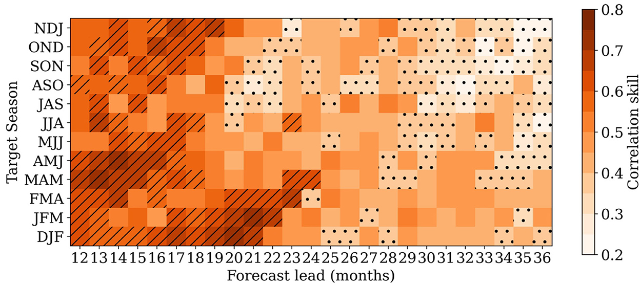
Figure 4. Same as in Figure 3A but up to a lead time of 36 months. Moderate to high correlations of 0.4–0.6 are noted at very high lead times, around 32 months. Correlation above 0.32 is statistically significant at a 95% level based on Student's 2-tailed t-test.

4.1.3. All season forecasted ENSO index

The time series of the observed, SINTEX-F2 predicted, and CNN predicted ENSO index along with the spread in the CNN ensemble members are shown in Figure 5. It is evident that seasonally varying CNN was successful in recording the peak ENSO events such as the El Niño of 1997/98, 2002/03, and 2009/10; and La Niña of 1988/89, 1999/00, 2010/11, and 2020/21. The SINTEX-F2 failed to predict most of those events. However, the CNN failed to capture the amplitude of the events correctly; although the amplitude of the forecasted ENSO index was underestimated, the phase was correctly predicted even at a longer time of 2.5–3 years (Refer to Supplementary Figure S1).

FIGURE 5

Figure 5. All season forecasted ENSO index from seasonally varying CNN models ensemble mean (blue), ensemble spread (shaded), SINTEX-F2 (orange) validated with observed OISSTv2 Nino3.4 index (black) at a lead time of 18 (A) and 23 (B) months. The validation period for the CNN experiment is 1984–2021 and SINTEX-F2 is 1985–2015. Correlation skills mentioned in the figures are statistically significant at a 95% level based on Student's 2-tailed t-test.

4.1.4. Peak and growth season forecasted ENSO index

We compared the forecasted ENSO index with those observed during peak (DJF) and growth Jun–Aug (JJA) seasons separately. As depicted in Figure 6, we notice a higher correlation skill in the predicted ENSO index during both peak and growth seasons at lead times of 18 and 23 months, as was seen for all season forecasted ENSO index. It is significant that the proposed CNN models are consistent in forecasting ENSO events during both growth and peak seasons, with a slightly improved skill for growth season at the 23-month lead time. On the other hand, in SINTEX-F2, though it is moderately better at 18 months, a further drop in the forecast skills is seen at 23 months' lead time during the peak season; with poor or no skills during the growth season. In addition, the winter season further demonstrates moderate correlation skills (0.43–0.39) for 2.5–3 years lead times with skills to forecast the El-Niño events of 1997/98, 2009/10, and 2015/16; and La-Niña events of 1984/85, 1999/00, and 2017/18 with slight underestimation in amplitude. Nonetheless, the growth season presents only reasonable to moderate skills at those lead times (Refer to Supplementary Figure S2).

FIGURE 6

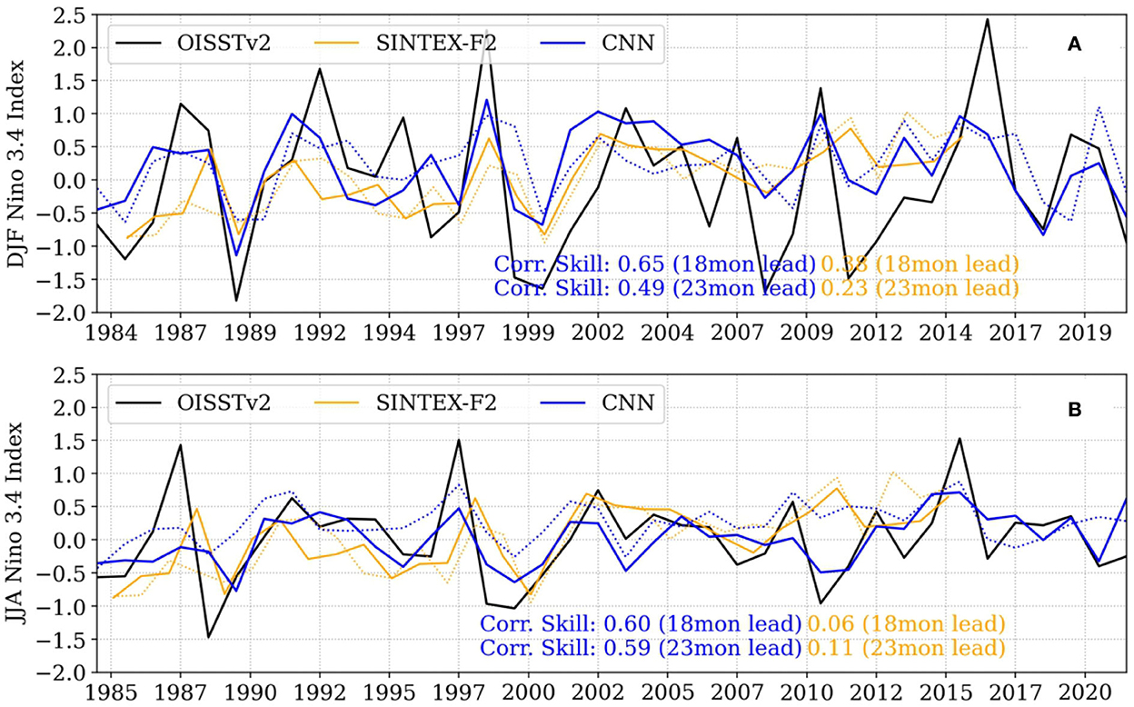
Figure 6. Time series of the ensemble mean forecasted ENSO index from seasonally varying CNN models (blue), SINTEX-F2 (orange) and validated with observed OISSTv2 (black) at lead time of 18 (solid) and 23 (dotted) months for (A) DJF and (B) JJA seasons. The validation period for the CNN experiment is from 1984 to 2021 and SINTEX-F2 is 1985-2015. Correlation skills mentioned in the figures are statistically significant at a 95% level based on Student's 2-tailed t-test.

5. Probabilistic skills

We further evaluated these models for their skills in probabilistic forecasts based on a relative operating characteristics (ROC) curve over the best ten ensemble members varying in initial conditions and internal CNN parameters. Figure 7 presents the probabilistic skills of all season forecasted ENSO index at 18- and 23-month lead times for El Niño, neutral, and La Niña events separated using a threshold of +0.5°C. ROC is plotted using hit rate and false alarm ratios, estimated by the number of events recorded vs. the total number of events that occurred, and the number of events wrongly forecasted vs. the number of nonevents, respectively, at various probability thresholds, as detailed in Mason and Graham (1999). The values in the ROC curve near the bottom-left indicate all ensemble members forecasting an event; thus, a high chance of an occurrence. Similarly, the values near the top-left indicate very few members forecasting an event; thus, a low chance of an occurrence. The overall probabilistic skill of the ROC curve is judged by the area under the ROC curve (AUC), the higher the AUC value highly, the more reliable the models are, and vice versa. Furthermore, the random predictions have an AUC of 0.5, as indicated by the black line in Figure 7. For a skill to be significant, it must be between 0.5 and 1.

FIGURE 7

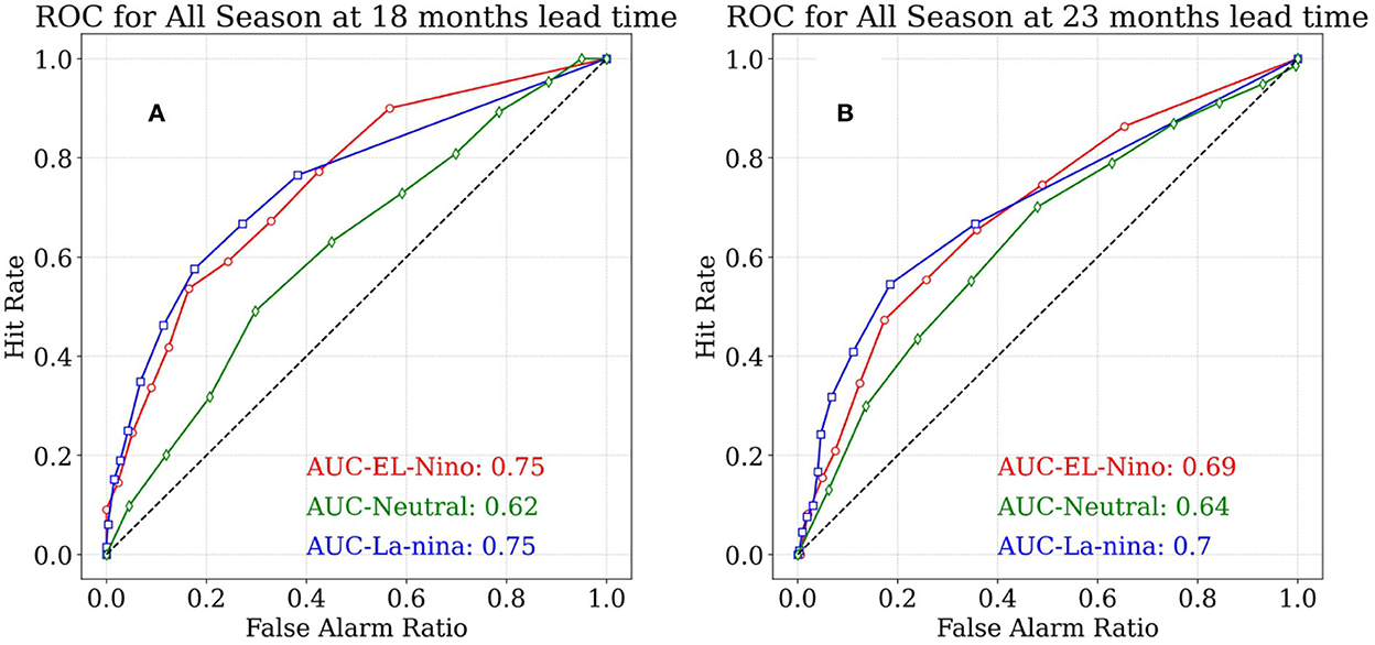
Figure 7. Probabilistic skill measured by ROC for various El-Niño (red), Neutral (black), and La-Niña (blue) events from all season forecasted ENSO index by seasonally varying CNN models at lead time of 18 (A) and 23 (B) months across various probability thresholds. An ensemble size of ten members is used for estimating the ROC. A threshold of ±0.5°C is used to separate various types of ENSO events. The dotted gray line indicates the probabilistic skills of random predictions. The procedure followed for calculating the hit rate and false alarms ratio is adopted by Mason and Graham (1999). Points to the left indicate many ensemble members capturing an event, whereas points to the right indicate very few members capturing an event in each panel.

Seasonally varying CNN models show high probabilistic skills at both lead times with a slight reduction at 23 months (Figure 7B). AUC for both El Niño and La Niña events is seen to be higher than 0.7 at both lead times, which is noteworthy, as El Niño events are comparatively difficult to predict compared to La Niña events (Philander, 1999; Luo et al., 2017). In addition, it is also important for models to forecast neutral events skillfully (Goddard and Dilley, 2005; Yu et al., 2010), wherein AUC for neutral events is >0.62 which is slightly lower than El Niño and La Niña events. However, skills are still substantially higher than the skills of random predictions. Moreover, very long lead forecasts up to 2.5–3 years show a moderate reduction in this skill compared with 18–23-month-lead times having an AUC >0.6 for El Niño, La Niña, and neutral events (Refer to Supplementary Figure S3).

6. Heatmap analysis

The above analysis indicates that the CNN model has good skills in predicting the ENSO index with a lead time of 1–3 years. In order to identify the regions of the global oceans that would have contributed to the skillful prediction of ENSO in the CNN model, we carried out a heatmap analysis of the seasonally varying CNN models. The heat map analysis was carried out for the extreme ENSO events. The heatmap analysis was performed for the first ensemble member among the best ten members for the third convolutional layer at 18- and 23-month lead times focusing on the boreal winter and summer. These heatmaps were based on the gradients (Equation 3) and activation maps (Equation 4) multiplied together at each region, better known as “‘GradCAM,” proposed by Selvaraju et al. (2020); refer to section Heatmaps of “Methods” for details. Darker regions in the heatmaps (Figures 8–11) portray stronger influences on the subsequent ENSO event.

FIGURE 8

Figure 8. Contribution of various oceanic regions estimated using GradCAM heatmaps (Selvaraju et al., 2020) for the best ensemble member among the top ten seasonally varying CNN models during growth (JJA) season ENSO index forecasting for strongest El-Niño of 1997, 2015 and La-Niña of 1998, 2020 with a lead time of 18 months (using NDJ season as predictors) (a–d) and 23 months (using JJA season as predictors) (e–h) estimated by multiplying Equation (3) and (4). Heatmaps (shaded) are estimated for the third convolutional layer. Darker shades indicate strong influence, with positively correlated shown in orange and negatively correlated in blue. Strong SSTA and VATA anomalies are overlapped on heatmaps with black and green contours, respectively, with solid lines for positive and dashed lines for negative values. The Tropical Pacific Ocean is highlighted by the black box.

6.1. Growth season (boreal summer)

We illustrate the contribution of various ocean regions using GradCAM heatmaps in Figure 8 to the growth season at 18- and 23-month lead times observed during the strongest El Niño events of 1997 and 2015 and La Niña events of 1998 and 2020. When compared to previous events, the 1997 El Niño was one of the strongest on record; predictors for the same were obtained from the Nov–Jan (NDJ) of 1995.

The prominent regions contributing to the 1997 El-Niño during the growth season were identified from the heatmaps as the Western Pacific, Southeast Pacific, Indian Ocean, tropical and subtropical southern Atlantic, and western hemisphere warm pool (Figure 8a). Similar regions were also noticed for the subsequent stronger El Niño event of 2015 (Figure 8c) when predicted from the NDJ-2013 at 18 months lead time, where the contributions from the Indian and Atlantic Ocean were relatively stronger with similar influence from the western Pacific. On the other hand, the contributors to the stronger La Niña events of 1998 (Figure 7B) and 2020 (Figure 7D) were of the opposite nature. Most of the influences come from similar regions when predicted by NDJ-1996 and NDJ-2018 at an 18-month lead time, with a weaker influence from the western Pacific and a stronger influence from the central Pacific. On the contrary, the contributing areas for the 23-month lead time are comparatively spread away from the western and central Pacific to the Indian and Atlantic Oceans with a stronger influence. For example, the Indian Ocean is strongly highlighted for 23 months lead time compared to the 18-month lead for La Niña of 1998 and 2020; El Niño of 2015; and the Atlantic Ocean for all the mentioned events (Figures 8e–h).

Interestingly, the roles of these mentioned regions are already identified in connection with successive ENSO developments in several past studies. This includes a negative (positive) dipole mode in the Indian Ocean triggering El Niño (La Niña) (Behera et al., 2006; Kug and Kang, 2006; Izumo et al., 2010; Luo et al., 2010). Negative (positive) surface anomalies in the Atlantic and subtropical Atlantic Ocean may lead to El Niño (La Niña) (Ham et al., 2013, 2021a; Zhang et al., 2019; Richter and Tokinaga, 2020) and positive (negative) surface anomalies in the western hemisphere warm pool potentially trigger El-Niño (La-Niña) (Park et al., 2018), surface anomalies in northern Pacific through Pacific meridional Mode (Chang et al., 2007), and surface and subsurface anomalies in the western to central Pacific preconditioning for various ENSO events (Ramesh and Murtugudde, 2012). Thus, the influential regions captured by the heatmap analyses in our study are supported well by the dynamical analysis in previous studies.

The precursors during the growth season were also analyzed from the first convolution layer at the 23-month lead time due to the stronger influence from the faraway Pacific region. An intriguing fact was distinguished in the Indian Ocean with a negative-dipole-mode-like structure as the only foremost precursor for various mentioned ENSO events, as depicted in Figure 9. Such a clear negative IOD-like pattern as a precursor to El Nino events was not captured by the heatmap analyses in previous studies (Ham et al., 2019, 2021b). A small disparity is observed though in this additional precursor analysis for La Niña events where the potential precursors were supposed to be the positive-dipole-like structure instead of the negative one.

FIGURE 9

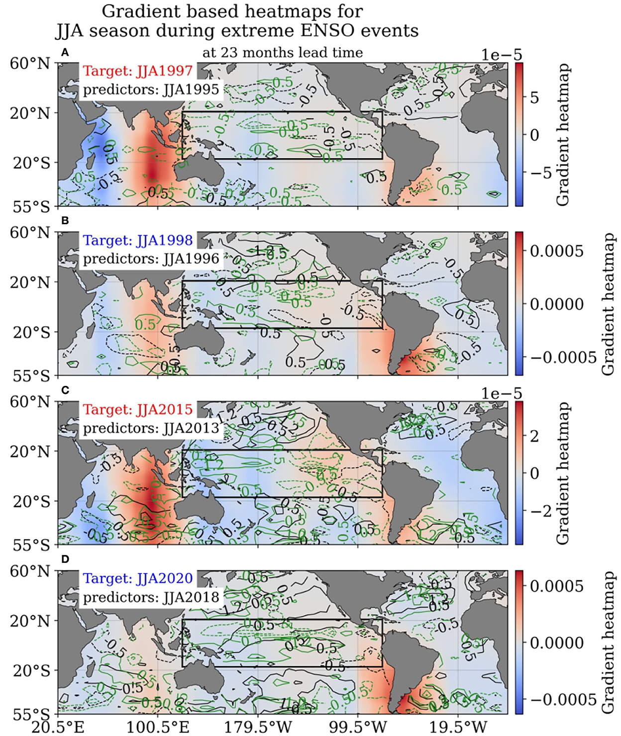
Figure 9. (a–d) Same in Figures 8e–h, but heatmaps are estimated using only gradients as in Equation (4) from the first convolutional layer at 23 months lead time.

6.2. Winter season

Potential precursors for the winter season were also observed for various stronger ENSO events, as shown in Figure 10. The nature of the precursor regions is similar to that seen during the growth season and at an 18-month lead time with predictors from the MJJ season. The major contributing areas for El Niño of 1997/98 (Figure 10A) and 2015/16 (Figure 10C) are highlighted as a negative-dipole-like structure in the Indian Ocean as well as anomalies in the western and subtropical Pacific, and subtropical Atlantic Ocean. The opposite nature of the precursors is seen for La Niña of 1998/99 (Figure 10B) and 2020/21 (Figure 10C). At the lead time of 23 months using the DJF season as the predictor (Figures 10E–H), the potential precursors were also noted in far regions of the tropical Pacific, Indian, and Atlantic Oceans. On the contrary, the influence of the tropical Pacific at a lead time of 23 months was also noted along with other regions unlike during the growth season. This contribution is attributed to the strong anomalies occurring in the tropical Pacific Ocean during the preceding peak season, which may be related to the biennial mode of ENSO variability (Rasmusson et al., 1990).

FIGURE 10

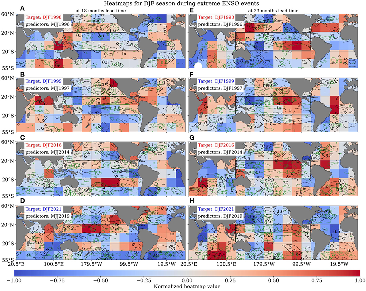
Figure 10. Heatmaps for highlighting the contribution of various oceanic regions for best ensemble member among the top ten seasonally varying CNN models during peak (DJF) season ENSO index forecasting for strongest El-Niño of 1997/98, 2015/6 and La-Niña of 1998/99, 2020/21 with a lead time of 18 months (using MJJ season as predictors) (A–D) and 23 months (using DJF season as predictors) (E–H). Heatmap estimation, shades, and contour meaning are the same as in Figure 7.

Similar to the growth season, we further analyzed the heatmap for the winter season at 30 months' lead time from the first convolutional layer. The results highlighted the south-western Indian Ocean as the main contributor. At the same time, the western hemisphere warm pool and northern tropical Atlantic Ocean were moderate contributors triggering successive ENSO events as seen in Figure 11. The anomalies in the south-western region can further grow in positive or negative Indian Ocean dipole mode events (Rao and Behera, 2005), which may further trigger the successive ENSO events (Izumo et al., 2010).

FIGURE 11

Figure 11. (A–D) Same in Figures 10A–D, but heatmaps are estimated using only gradients as in Equation (4) from the first convolutional layer at 23 months lead time.

7. Discussion

The forecast skill of seasonally varying CNN models is found to be better than those of the fixed-parameter CNN, SINTEX-F2 dynamical model, and previous deep learning-based ENSO predictions (Ham et al., 2019, 2021a; Geng and Wang, 2021; Hu et al., 2021; Liu et al., 2021; Mu et al., 2021). Despite the higher forecast skills observed in our CNN models for all season forecasted ENSO index and its seasonal variation, the amplitude of the ENSO index in the ensemble mean was underestimated (Figure 5). Such an underestimation is likely due to the selection of the best ten members for making the ensemble mean. As can be seen in Figure 12, indeed a few members, among the best ten, are capable of catching the peak of extreme ENSO events. Such an underestimation is common in statistical schemes and is also observed in preceding studies applied to ENSO forecasting (Yan et al., 2020; Geng and Wang, 2021; Hu et al., 2021; Mu et al., 2021). Furthermore, such underestimation can be corrected using a suitable bias correction technique (Eade et al., 2014), provided that the observed and forecasted indices are highly correlated, as shown in Figures 5, 6.

FIGURE 12

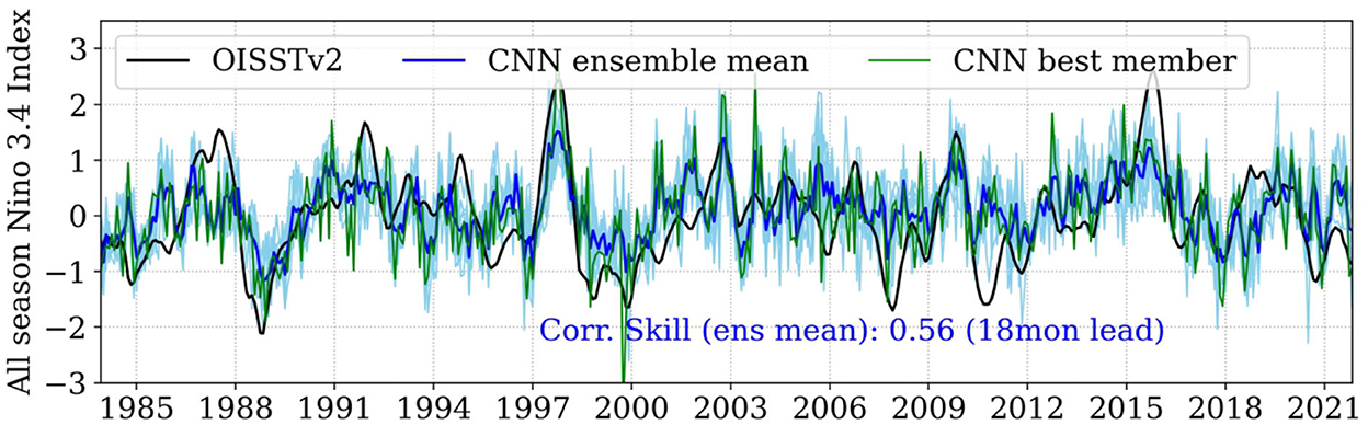
Figure 12. All season forecasted ENSO indexes from seasonally varying CNN models for the ensemble mean (blue), best ensemble member (green), and individual ten ensemble members (light blue) validated with observed (OISSTv2, black) index over a period from 1984 to 2021 at a lead time of 18 months. Despite the underestimation in the ensemble mean, few ensemble members are seen significantly capturing the amplitude of important ENSO events. Correlation skills mentioned in the figure are statistically significant at a 95% level based on Student's 2-tailed t-test.

Apart from the underestimation, the forecasted all-season ENSO index was found to miss a few important events, including the El Niño of 2015/16, La Niñas of 1998/99, 2007/08, 2010/11, and the recent 2020/21 (Figure 5). Nonetheless, these missed events were found to be reasonably captured either during the growth/peak season by the ensemble mean (Figure 6) or by one of the ensemble members with substantial skill (Figures 12, 13).

FIGURE 13

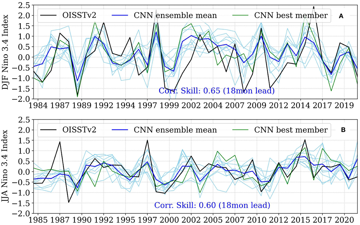
Figure 13. Same as in Figure 12 but for the DJF (A) and JJA (B) seasons. Correlation skills mentioned in the figures are statistically significant at a 95% level based on Student's 2-tailed t-test.

In addition to the improvements in deterministic skills, our CNN models do show noteworthy skills in probabilistic forecasts. AUC for various types of ENSO events was found to be significantly higher at 18- to 23-month lead times and to have reasonable to moderate skills at 30- to 36-month lead times. The AUC for El Niño events was sometimes found to be higher compared to that of the La Niña events. Such skills will greatly benefit from being able to reliably forecast stronger El Niño events, which may occur more frequently in future decades due to climate changes (Timmermann et al., 1999; Cai et al., 2014; Wang et al., 2017; Freund et al., 2020). Furthermore, the probabilistic skills mentioned above were based on the +0.5°C threshold used to separate different types of ENSO events; it is interesting to note that such skills are least disturbed when the threshold is increased to +1.0°C (Refer to Supplementary Figure S4).

Heatmap analyses suggest that the precursors are widely spread in the world's oceans. Though most precursors were in the tropical Pacific, significant precursors also manifested in the Indian and Atlantic Oceans much prior to ENSO occurrences. Moderate to significant contributions (Figure not shown) came from the tropical Pacific at a lead time of 23 months; such contributions were also noted by Ramesh and Murtugudde (2012) when they analyzed precursors of ENSO at an 18-month lead time, suggesting the intrinsic precursors of ENSO may largely be buried inside the tropical Pacific. Indeed, a separate numerical study is required to support such an analysis of the ENSO precursor at a very long lead time of 30–36 months. Furthermore, the Indian Ocean emerges as one of the main contributors to successive ENSO events. As noted in additional heatmaps analysis performed for long (23 months) (Figure 9) and very long (30 months) lead times (Figure 11), obvious patterns of negative Indian Ocean dipole are observed with regions in the south-western Indian Ocean during the growth and winter seasons, coinciding with stronger SSTA and VATA.

8. Conclusion

The present study demonstrates the potential of CNN models to accurately forecast ENSO events at long lead times of up to 2 years in all seasons and further up to 3 years for the winter season. Such ENSO forecasts are also found to greatly outperform the state-of-the-art dynamical model SINTEX-F2 and previous deep-learning approaches. The proposed CNN models are also efficient in forecasting the important extreme ENSO events during the seasons of interest. Such forewarning of ENSO events is extremely important as these extremes are considered to occur more frequently in the near future (Cai et al., 2014). However, the tropical Pacific Ocean provides the majority of forecasting skills with a 2-year lead time. Regions in the Indian, Atlantic, and tropical Pacific Oceans are found to be responsible for the generation of successive ENSO events. In particular, substantial contributions come from the Indian Ocean at longer lead times of 2–3 years. In conclusion, this study shows that CNN is a prospective tool for providing skillful ENSO forecasts relative to the current dynamical systems and can investigate possible precursors.

Data availability statement

The datasets used for training and validating the proposed CNN models are openly available. COBEv2 SST data is obtained from (https://psl.noaa.gov/data/gridded/data.cobe2.html). SODA v2 and GODAS datasets are acquired from (http://apdrc.soest.hawaii.edu/datadoc/soda_2.2.4.php) and (http://apdrc.soest.hawaii.edu/datadoc/godas_monthly.php). OISSTv2 data is available from (https://psl.noaa.gov/data/gridded/data.noaa.oisst.v2.html). The outputs of SST from the SINTEX-F2 dynamical model were furnished on request by Dr. Takeshi Doi, APL, JAMSTEC, please contact on takeshi.doi@jamstec.go.jp.

Author contributions

KP, TD, VJ, and SB contributed to the study's conceptualization, article writing, and findings interpretation. TD performed the SINTEX-F2 dynamical model setup and predicted global SSTA. KP was in charge of CNN modeling and analysis. All authors contributed to the article and approved the submitted version.

Funding

KP is appreciative of the financial support provided by the JAMSTEC young research award to carry out this study.

Acknowledgments

KP gratefully welcomes the financial assistance provided by the JAMSTEC young research grant as well as the computational assistance supplied by Earth Simulator by JAMSTEC in order to complete this project. The authors also want to thank the reviewers for their insightful feedback on the manuscript. The authors also thank Python, Keras, and Tensorflow developers for contributing open-source libraries.

Conflict of interest

The authors declare that the research was conducted in the absence of any commercial or financial relationships that could be construed as a potential conflict of interest.

Publisher's note

All claims expressed in this article are solely those of the authors and do not necessarily represent those of their affiliated organizations, or those of the publisher, the editors and the reviewers. Any product that may be evaluated in this article, or claim that may be made by its manufacturer, is not guaranteed or endorsed by the publisher.

Supplementary material

The Supplementary Material for this article can be found online at: https://www.frontiersin.org/articles/10.3389/fclim.2022.1058677/full#supplementary-material

References

Abadi, M., Agarwal, A., Barham, P., Brevdo, E., Chen, Z., Citro, C., et al. (2016). Tensorflow: Large-scale machine learning on heterogeneous distributed systems. arXiv preprint arXiv:1603, 04467.

Google Scholar

Alexander, M. A., Bladé, I., Newman, M., Lanzante, J. R., Lau, N. C., and Scott, J. D. (2002). The atmospheric bridge: the influence of ENSO teleconnections on air–sea interaction over the global oceans. J. Clim. 15, 2205–2231. doi: 10.1175/1520-0442(2002)015<2205:TABTIO>2.0.CO;2

ORIGINAL RESEARCH article

Deep learning for skillful long-lead ENSO forecasts

1. Introduction

2. Datasets

3. Model and methods

3.1. Proposed CNN architecture

3.2. Customized loss function to train the CNN

3.3. Seasonally varying internal CNN parameters

3.4. Heatmaps

3.5. SINTEX-F2 dynamical prediction system

4. Results

4.1. Deterministic skills

4.1.1. Multi-year all season ENSO index correlation skill

4.1.2. Seasonal variation of correlation skill

4.1.3. All season forecasted ENSO index

4.1.4. Peak and growth season forecasted ENSO index

5. Probabilistic skills

6. Heatmap analysis

6.1. Growth season (boreal summer)

6.2. Winter season

7. Discussion

8. Conclusion

Data availability statement

Author contributions

Funding

Acknowledgments

Conflict of interest

Publisher's note

Supplementary material

References

This article is part of the Research Topic

People also looked at