Climate-change scenarios require volatility effects to imply substantial credit losses: shocks drive credit risk not changes in economic trends

1. Introduction

Due to recent increased concerns over the long-term effects of climate change, regulators in several jurisdictions have worked with banks to assess climate stress tests (“CST”) for both the possible effects of climate change on their clients and the financial losses that a bank might incur as a consequence to those effects on company debt levels. Some regulators notably the ECB/ESRB and Project Team on Climate Risk Monitoring (2021) working with the NGFS (2022a,b) have proposed that banks try to identify the credit losses associated with a range of “top–down” style scenarios involving varying amounts of mitigation and climate-change intensities. While the NGFS scenarios are “top–down,” they are applied to individual companies on a “bottom-up” basis to assess scenario impacts on levels of debt and associated company probabilities of default (“PD”).

In most of these climate scenarios as currently applied, climate change slows economic growth, but does not affect the cyclical variability of the factors influencing credit risk. As a result, climate change in these scenarios has little impact on credit losses. This unsurprising result, is in contrast, to potentially larger climate change impacts that produce more (volatility) through extreme, weather events, related larger, political, or economic unexpected future shocks, that yields more severe physical-damage and higher economic and social costs. The lack of larger credit risk impacts in current CST efforts can also be contrasted with current, traditional, short-run regulatory capital stress testing that, in extreme (adverse) scenarios does impart larger economic shocks through sudden impacts on company cashflows.

Some of these recent CST studies, notably those from the Alogoskoufis et al. (2021) and ECB/ESRB and Project Team on Climate Risk Monitoring (2021), trace climate-change's effects on companies to rising costs caused by greater physical damage, more stranded carbon assets, and higher carbon taxes. Those studies use a key assumption that see these cost increases as incompletely passed through in prices. Thus, company profit margins decline and in response default rates and credit losses rise. However, under the alternative view that long-run cost increases are typically fully passed through in firm's output prices, the credit effects would for the most part be potentially small. The gradual decline in output growth and the slow progression of cost increases as usually represented in mainstream economic models, offer businesses ample time to adapt. But in contrast, in most credit models, only unanticipated shocks produce material increases in observed defaults and credit losses.

Here, we show that if, contrary to the NGFS scenarios, climate change increases the volatilities of systematic, credit-risk factors, then, in more severe climate scenarios, deeper credit downturns and higher credit losses could occur. Therefore, any assessment of future climate induced credit risks must assess systematic volatility not just trends in economic variables such as GDP. Luckily there is substantial objective and empirical evidence on credit cycles available from the last 40 years and a credit-factor framework to assess credit risk volatility, that can also be complementary to early CST approaches.

Recently in discussions and feedback concerning the primary NGFS CST scenario approach there is also a growing industry discussion concerning a set of more general points related to the application of these primarily top-down, smooth, scenario-based approaches. These include:

(1) The use of deterministic scenarios that are based on quite limited objective, empirical data,

(2) Application of IAM-derived mostly “smooth trend-like” scenarios—these don't include the usual drivers of systematic credit risk “shocks,”

(3) A lack of incorporation of more extreme near-catastrophic future “states of the world,” which limits NGFS assessments of potential extreme climate risks, and their related, potential probabilities, and,

(4) A limited ability to assess granular risk, as “top down” approaches cannot assess detailed industry and financial sector behavior.

Climate risk impacts are highly uncertain and assessing future credit risks over long 30-year or more horizons is a quite complicated task. The current CST NGFS scenario-focus generally seems to stem from the lack of, measurable, historical climate impacts on detailed economic, financial and industry sector data. Therefore, regulators and the NGFS have developed “stylized” scenarios derived from simplified “top–down” models. These NGFS scenarios provide a good start to thinking about long-run financial impacts of climate change as well as a standardized framework that can be applied in individual regulatory jurisdictions. However, current historical climate data limitations are one key constraint that limits the ability to better assess climate uncertainty and develop more empirical, statistical analysis including assessing implied probabilities of extreme climate scenarios.

In the context of developing risk models generally, the goal is focused on assessing an unbiased range of potential future outcomes and estimating (as best as possible) related empirical probabilities for these potential future outcomes. Adding more extreme, complex long-run climate scenarios are a contribution to developing a more unbiased “candidate set of possible future, climate and risk outcomes.” In the current, general NGFS CST approach, while good progress has been made, the NGFS approach seems to lack, both of these aspects inherent in general risk prediction models. Specifically, the inclusion of a wider unbiased candidate set of potential future “climate states of the world” coupled with related probabilities developed at least in a reasonably objective, empirically based way.

In this paper, we briefly review these key climate stress test discussion points but focus primarily on the role of systematic volatility. We present three climate risk assessments using the empirically based credit-factor framework we have developed in the Z-Risk Engine (“ZRE”) portfolio solution (Chawla et al., 2016; Forest and Aguais, 2019a,b,c).¹ The credit-factor approach applied in these assessments has been developed over the last 15 years and is well documented in the literature, and is developed from credit factors estimated from the full history of Moody's CreditEdge EDFs, (Nazeran and Dywer, 2015;Moody's Analytics, 2016). A similar approach to applying credit-factor simulations to assess climate risk can also be found in Garnier et al. (2022).

In the first assessment we compare the NGFS scenarios with the CCAR (Severely Adverse Capital Stress) scenario produced by the US Federal Reserve (Board of Governors of the Federal Reserve System, 2022b).² To accomplish this we apply the ZRE Scenario Forecasting Model (“SFM”) utilized to assess deterministic scenarios such as the NGFS and CCAR scenarios. The SFM starts with predetermined, macroeconomic-variable (“MEV”) scenarios, transforms MEVs into credit indicators called MEV Zs, and the approach then bridges from those MEV Zs to industry and region Zs, and through a series of further steps obtains credit-loss scenarios for a benchmark portfolio of corporate and commercial exposures.³ See Section 5 for more details.

The second assessment applies the ZRE Industry Region Monte-Carlo (“IRMC”) model, which begins with Monte Carlo simulations (“sims”) of the industry and region systematic factor Zs that in turn, through a series of further steps, leads to portfolio, credit-loss distributions. The third assessment, referred to as the Scenario-Forecasting, Monte-Carlo (“SFMC”) model, adds a Monte Carlo simulation engine for the MEV Z factors to the SFMC just described and thereby produces alternative credit-loss sims. Applying these models in estimating the credit losses of a hypothetical portfolio representative of US bank, commercial-and-industrial (C&I) loans, we find that, only after making credit-factor volatilities sensitive to global warming, do more severe, climate scenarios imply substantially higher credit losses, especially in downturns.

The climate-sensitive results in this paper involve an assumed relationship between global mean temperatures (GMTs) and credit-factor volatilities. Thus far, we have no empirical results to substantiate this or any other relationship between a climate metric and credit-factor volatilities. As additional research not included here, we have compared the CCAR series on market volatilities with GMTs and have found an insignificant (but positive) correlation. Thus, the quantitative results presented here for the direct GMT climate impacts remains illustrative, however the credit-factor models applied to assess these hypothetical climate impacts on credit losses is empirically based.

To highlight the key, new contributions presented in this paper, the empirical application of the macro-factor model discussed in more detail below juxtaposes NGFS scenarios with a CCAR scenario to highlight discussion point (1) in the literature that the current NGFS scenarios lack a more objective empirical foundation. The application of the CCAR scenario comparison also highlights concerns expressed above about the NGFS approach lacking the ability to apply unexpected systematic shocks consistent with past economic discontinuities as highlighted in discussion point (2). Applying long-run shocks for climate stress testing is key given the large uncertainty and the potential for higher future volatility as outlined, relating to major climate change.

The paper also runs detailed, empirical macro and industry/region credit-factor model assessments of climate risk impacts on credit losses whose results provide more clarity on discussion points (3) and (4), by assessing statistical “tail” climate related credit losses and applying detailed, dedicated industry/region factor models. Both assessments make new contributions to the climate change CST literature.

2. Brief review of current climate stress testing literature

Climate stress testing is a quite new topic, generally, and most research and articles have been published over only the last roughly 5 years. This includes the key focus on this topic by regulators. In this brief literature review, we highlight key recent contributions on two threads in the literature: the application of climate financial impact analysis in assessing company-specific climate impacts on PDs, and recent, related work by the regulators and the global NGFS consortium. We also link the four key industry discussion points we cited in the introduction to the related literature to set the context for the primary contributions of this paper focused on applying a more elaborate credit risk framework to assess climate change impacts.

Enhanced general stress testing of bank regulatory capital by financial regulators over the last roughly 20 years has been part of the overall Basel financial regulatory efforts to reform and enhance the global rules regarding bank capital and therefore overall macro-financial stability. For credit risky assets within banks, this effort has included the implementation of various regulatory enhancements to the core credit models (probability of default, loss-given default and exposure-at-default) used by banks. These efforts around the world have been substantial and form the enhanced foundation on which regulators oversee banking capital and risk management in banks.

The specific focus by regulators in conjunction with the banks they oversee on CST has only really become part of the overall climate change landscape in the last 3–5 years. This means that, CST models, methodologies and various sources of climate data to support CST are all in a very early stage of discussion and development. To support this global effort, the NGFS (“The Network of Central Banks and Supervisors for Greening the Financial System”) was formed in late 2017 following the 2015 Paris Climate Agreement. The NGFS is an umbrella, voluntary, cooperative organization focused on sharing best practices on the relationship between the environment and the development of climate risk management frameworks for the financial sector. Research efforts by the NGFS have therefore supported the development of a “common scenario-based” framework that forms the foundation generally of early CST research and modeling.

Focusing specifically, on recent key CST publications, see Battiston et al. (2017) for an initial framework for assessing climate impacts on financial asset classes, for European equities and debt, through the application of a “Climate VaR” approach. This research like other recent climate analysis applies a network approach to assess direct and indirect climate effects on a portfolio of financial assets. Focusing on climate impacts on financial assets, Battiston et al. (2019) assessed “pricing forward-looking climate risks under uncertainty.” Climate risk modeling based upon a Merton-Style company default model Baldassarri Höger von Högersthal et al. (2020), assessed various carbon price, price elasticity and cost pass-through assumptions of climate change on public-company PDs. The focus on Merton-style PD approaches across various time horizons, can also be found in Bouchet and Guenedal (2020), Capasso et al. (2020), and Adenot et al. (2022).

Key contributions from the regulators in recent years, include work by the Dutch Central Bank, Vermeulen et al. (2021) who focused on the aggregate Dutch Banking System, in applying a “topdown” stress test approach centered on various “shocks” including carbon price and technology shocks. From the French Regulators, Allen et al. (2020) also develops a CST approach for the French Banking System.

On the overall NGFS approach, see Boirard et al. (2022) and Monasterolo et al. (2022), for a general discussion, and NGFS (2022a, b). These models utilize primarily top-down scenarios, with the scenario approach motivated generally like others by very high levels of future climate uncertainty over long time horizons coupled with a lack of historical data available to build detailed empirical, predictive CST models.

Focusing on the four key industry discussion points, as pointed out in Aguais (2022), using the Rumsfeld risk taxonomy, climate risk is usually thought of as a “known–unknown.” What is “known” is that broad measures of global temperature (driven by CO₂ levels) most likely will increase and climate change policy responses have the potential to substantially impact carbon usage (carbon asset stranding) and economic and financial activity globally (GDP). Increasing severe weather volatility which is creating physical climate risk is already being observed.

What is “unknown” is how much these broad measures of potential temperature change and atmospheric CO₂ will impact GDP globally, economic activity generally, future volatility, and society overall. Future carbon policy in the form of carbon pricing primarily and future technology changes in energy markets could make positive contributions to the climate transition but remain highly uncertain. Climate change is fundamentally embedded in the last roughly 50–60 years of observed economic and financial data—but detailed statistical measures of climate impacts are hard to directly extract to calibrate better climate credit risk models.⁴

Narrower physical climate impacts through measured CO₂ emissions, rising global mean temperatures and increasing severe weather volatility are generally observable, but highly uncertain over long run horizons. Therefore, any climate risk assessments are dominated by large uncertainties over the long-run horizons currently under discussion. As already highlighted, credit risk in principle is driven by unexpected economic shocks not smaller deviations to trend variables like mean temperature and CO₂ levels. Finally, substantial climate uncertainty is also assessed to have “fat tails” (Wagner and Weitzman, 2015).

Scenario-based approaches however have their own limitations, as they are ultimately hard to validate because they basically represent “what if,” usually deterministic, views of possible future states of the world (Hughes, 2021a,b, 2022). CST approaches are also usually driven top-down primarily, focused on IAM-style models which also have a hard time assessing disaggregated sectors in detail (Pitman et al., 2022).⁵,⁶,⁷

Current CST approaches not only have a hard time “distributing climate risk” to lower levels—as has been pointed out Aguais (2022) and Cliffe (2021)—in addition, Kemp et al. (2022) also states; “prudent risk management requires consideration of bad-to-worse-case scenarios…for climate change, such potential futures are poorly understood…could anthropogenic climate change result in worldwide societal collapse or even human extinction?”⁸

The recent Real World Climate Scenarios (Cliffe, 2022; Cliffe et al., 2022) roundtable has elaborated on some of these concerns suggesting that better and more detailed “climate narratives” should also be part of enhanced CST approaches.⁹

Khanna (2022) has recently asked, “What Comes After the Coming Climate Anarchy?” suggesting potential extreme scenarios could have substantially negative impacts. David Wallace-Wells highlighted potential long-run existential concerns at plus 6 degrees C or more in the Uninhabitable Earth (Wallace-Wells, 2019). Kemp et al. (2022) also express substantial concerns about the lack of inclusion of catastrophic scenarios, stating: “climate catastrophe is relatively under-studied and poorly understood…cascading impacts are underexamined” (see text footnote 8).

The ultimate existential metaphor for the potential impact of climate change uncertainty was developed in the 2021 Paramount film, “Don't Look Up”—we call this the “DiCaprio Scenario”, (McKay, 2021). Overall, building on early CST work requires a much “broader” range of possible future risks—however, Stern et al. (2022) suggest including a “DiCaprio Scenario” for the end of the world would usually make CST models intractable.

Overall, the recent extensive research supporting climate stress testing, as outlined above, has focused mostly on, “stylized” deterministic, standardized scenarios developed by the NGFS consortium. Our three climate stress test assessments presented in this paper are meant to provide complementary ways to assess these key topics, adding to the overall debate by focusing on more detailed approaches to assessing systematic credit risks and the impacts of climate volatility.

3. Assessing NGFS and CCAR scenario credit losses using an empirical multi credit-factor approach

3.1. Overview of multi credit factor approach

For the empirical results presented in this article we apply various modules of the Z-Risk Engine (www.z-riskengine.com) multi credit-factor portfolio model to a benchmark C&I USA credit portfolio generally designed to replicate the indices reported by the FRB (Board of Governors of the Federal Reserve System, 2022a). The ZRE portfolio credit-factor approach was developed to support assessments of both Point-in-Time (“PIT”) and Through-the-Cycle (“TTC”) credit measures for Basel capital, stress testing and IFRS9.¹⁰

In implementing MEV-based Z indexes as presented below for the first assessment, we also translate GDP into a credit-cycle indicator, which requires one to first de-trend it. We accomplish that here by forming the ratio of GDP to an AR1 moving average of GDP. In this ratio, the moving average represents a debt proxy. Thus, GDP over its moving average corresponds roughly to cash flow over debt or debt service. For other credit-related series, we perform similar transformations before adding the normalizations that produce credit-cycle, Z indexes. See Section 5 for more detail.

3.2. NGFS climate scenarios imply uniformly small, credit losses

The first credit risk assessment presented focuses on comparing GDP projections from various NGFS scenarios to the well-known CCAR capital stress scenario to highlight the role of unexpected shocks. Applying the ZRE SFM we find that the NGFS scenarios imply credit losses that are small compared with those realized in past recessions. Further, the differences in losses estimated for moderate and severe, climate scenarios fall short of the differences estimated for regulatory baseline and stress scenarios. Thus, based on the climate scenarios now available, climate-change appears to have relatively little effect on credit losses.

We attribute these findings to the smoothness of the NGFS scenarios. The scenarios differ in economic growth rates but show little volatility around long-run trends. Evidently the scenarios seek to describe the long-run, welfare (consumption) losses related to climate change and not any systemic instabilities. But successful, credit models trace most defaults and losses to sharp declines in asset values and cash flows relative to trend and not to gradually slowing trends.

3.3. Large credit losses occur occasionally and suddenly

Experience indicates that credit crises arise in the manner described by Dornbusch's Law¹¹:

“The crisis takes a much longer time coming than you think, and then it happens much faster than you would have thought.”

Paraphrased for credit, one might state this as follows:

“Credit crises occur only occasionally, but, when they do, they happen suddenly, caused by sharp declines in asset values or cash flows relative to debt or debt service.”

We see the pattern of intermittent, large credit risk events in the history of US C&I credit losses assessed by the FRB. Over the past 32 years, C&I losses have risen sharply three times, in 1990–1991 and especially 2001–2002 and 2008–2009, with each episode lasting about a year (see Figure 1). About half of past, C&I, credit losses trace to these roughly once-a-decade, major spikes. During the 2020–2021, COVID-19 induced recession, loan losses rose only moderately, perhaps due to forbearance inspired by the recognition that the downturn involved a necessary pause rather than fundamental failure of some businesses.

FIGURE 1

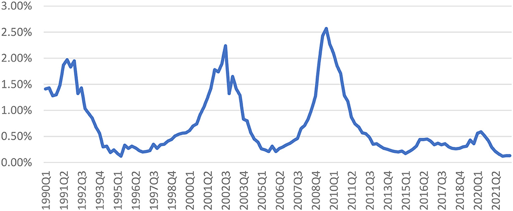
Figure 1. Annualized charge-off rates (%), US C&I loans, quarterly, seasonally adjusted. Source: board of governors of the federal reserve system.

3.4. NGFS scenarios show climate change as affecting economic trends and not volatility

The NGFS scenarios specify slightly different GDP growth rates in different climate scenarios (Table 1). However, the scenarios only indicate that growth rates may differ, but say nothing about cyclical instabilities around growth trends. To obtain quarterly projections, we must also resort to interpolation—the result; extremely smooth GDP scenarios.

TABLE 1

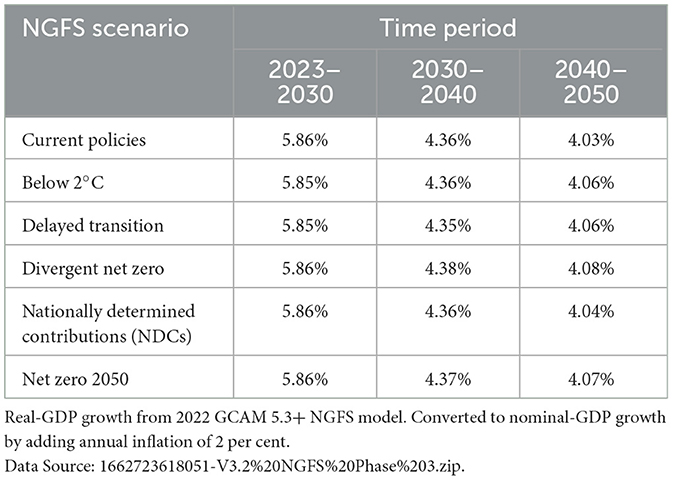
Table 1. Annual GDP growth rates in NGFS scenarios.

3.5. NGFS scenarios imply uniformly smooth credit-factor scenarios

Transformed into quarterly, credit-cycle, Z indexes for GDP, we get extremely smooth, credit-risk scenarios showing no major downturns and immaterial differences across scenarios (Figure 2). One sees very little difference between the severe climate-change, Current Policies Scenario and the moderate climate-change, Net Zero 2050 one. In contrast, the 2022 CCAR Severely Adverse Scenario has a strikingly different profile, exhibiting large deviations from the average setting of zero and from the baseline (no stress) scenario. While we don't show it here, the 2022 CCAR Baseline Scenario implies a Macro-Z path that sits almost on top of the NGFS Macro-Z paths.

FIGURE 2

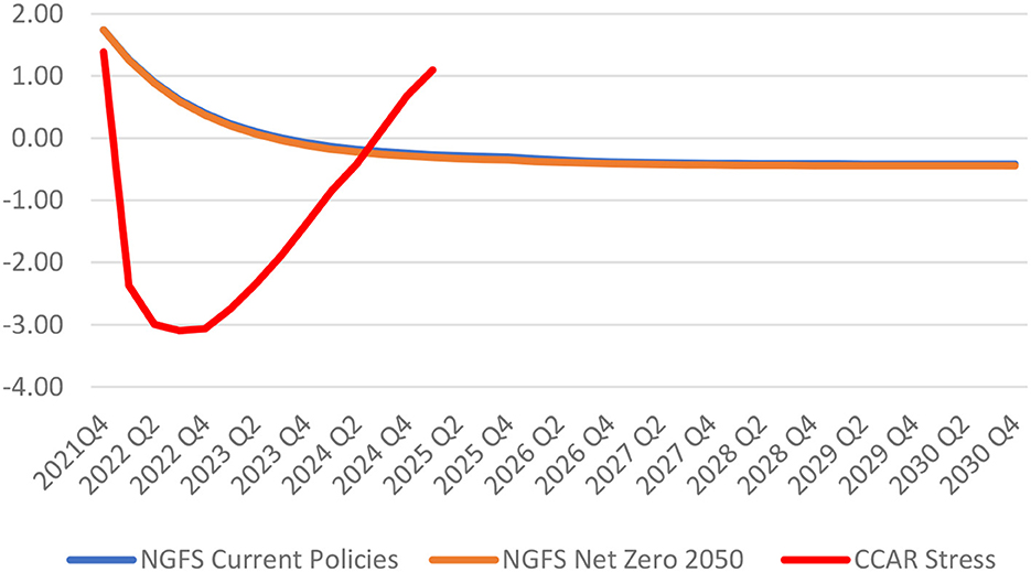
Figure 2. US macro credit-factor paths under CCAR and NGFS scenarios. Source: board of governors of the federal reserve system and Z-risk engine, NGFS.

3.6. Low volatility NGFS credit scenarios imply uniformly small, credit losses

Entering these scenarios into the SFM applied to a representative, C&I portfolio, we find that the NGFS scenarios imply uniformly small losses, with charge-off rates staying below the 1990Q1–2022Q2 average of 0.72%. In striking contrast, the 2022 CCAR Severely Adverse Scenario implies very large losses, with charge-off rates rising to more than 3x the historical average, see Figure 3.

FIGURE 3

Figure 3. Estimated, C&I charge-off rates: CCAR and NGFS scenarios. Source: board of governors of the federal reserve system, NGFS and Z-risk engine.

As a secondary factor explaining the insensitivity of losses to the NGFS scenario, those scenarios provide only GDP projections as possible credit factors. The historical record indicates that GDP is mostly a through-the-cycle (TTC), credit indicator, not explaining much of the past variation in observed default and loss rates. When running SFM we generally find empirically that the best predictors of observed credit losses are credit spreads and equities along with GDP. As shown in Section 5, in applying the SFM “Bridge” model, the application of the CCAR scenario uses all three macro-economic indicators, (spreads, equities and GDP) while applying the NGFS scenarios uses only GDP.

4. Adding climate-change volatility multipliers to credit models

The above discussion suggests that, to have a substantial effect on credit losses, climate change must generate greater volatility in the factors driving credit risk. Higher potential future climate driven volatility is expected in general and could be driven by a range of factors from; increasingly severe weather and physical damage, abrupt carbon policy changes, social and population migration and war “tipping points”—our application of volatility multipliers driven by projected GMT increases should be considered an aggregate measure of all of the future uncertain drivers of climate change. This allows us to illustrate the statistical impacts of future volatility on credit risk from the potential impact of climate and to also develop statistical probabilities attached to a given scenario.

We introduce this into the IRMC and SFMC models by applying climate-sensitive multipliers to the random, Z shocks underlying credit risk. We express these multipliers as a function of global mean temperature (GMT). As GMT rises, the volatilities of shocks increase, contributing to a wider range of Z outcomes. GMTs vary across the different climate scenarios and this implies different, volatility multipliers (Figures 4, 5). We calculate the climate-change, volatility multipliers (CMs) using the formula:

$\begin{array}{l}C{M}_t={\left(1+\frac{(GM{T}_t-GM{T}_{2020})}{14.5}\right)}^4.\end{array}$

Explanation of GMT/Vol formula: 14.5 C is approximately the average GMT over 1990–2020 (NASA, 2020). That's 13.9 C (approximate pre-industrial GMT) + 0.6 C average anomaly over 1990–2020. Thus, the vol-multiplier formula expresses the increase in GMT since 2020 in each simulation quarter as a ratio to the 1990–2020 average GMT. Then the formula raises that ratio to the fourth power.

FIGURE 4

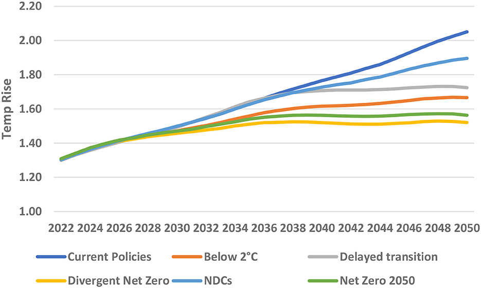
Figure 4. GMT anomalies in NGFS scenarios. Source: NGFS and Z-risk engine.

FIGURE 5

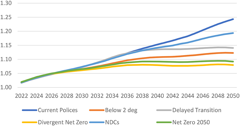
Figure 5. GMT-implied volatility multipliers in NGFS scenarios. Source: NGFS and Z-risk engine.

4.1. Volatility multipliers produce higher credit losses related to climate change

Applying alternatively the climate-sensitive, IRMC and SFMC models, we've run 1,000 loss sims from 2022Q2 to 2050Q4 for each of the following climate scenarios: Baseline (no climate effects); NGFS Net Zero 2050; NGFS Delayed Transition; and NGFS Current Polices. The Baseline involves no volatility multipliers, whereas the other three include the multipliers displayed above (Table 2, Figure 5). In these sims, we've estimated credit losses for a portfolio representative of US, C&I loans.

TABLE 2

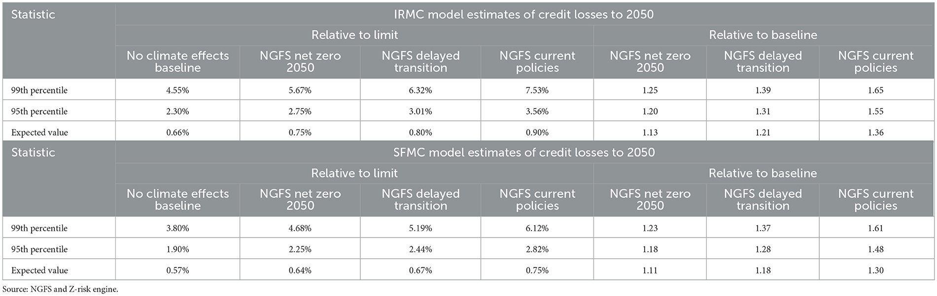
Table 2. IRMC and SFMC model estimates of credit losses for portfolio representative of US, C&I loans.

The results for the year 2050 show that credit losses increase as climate change and the volatility multipliers rise above one in the application of both the IRMC and SFMC models predicting credit losses. We also see that the climate effects become greater in the upper tail of the loss distribution. Thus, as estimated by the IRMC model, the expected credit losses in the NGFS Net Zero 2050, NGFS Delayed Transition, and NGFS Current Policies scenarios rise relative to the baseline by 1.13 × , 1.21 × , and 1.36 × , respectively. The 99th percentile losses in those scenarios rise relative to the baseline by 1.25 × , 1.39 × , and 1.65 × , respectively. The SFMC model produces similar results, but the loss estimates particularly at high percentiles fall below those from the IRMC model (Figure 6).

FIGURE 6

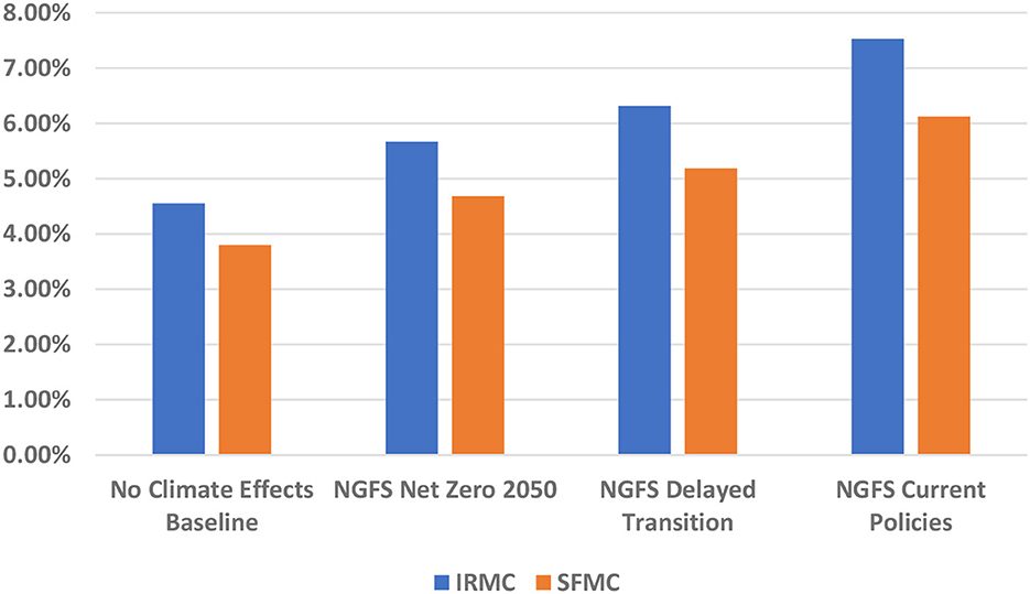
Figure 6. Alternative model estimates of 99^th percentile losses in 2050. Source: NGFS and Z-risk engine.

For broad comparison purposes, the 2008/2009 “Great Recession” produced a roughly 2.3% realized credit loss rate for 2009 as measured by the FRB C&I index. For 2002, the realized credit loss rates were about 1.8% vs. the 1990–2022 average C&I credit loss rate from the FRB index of about 0.72%. Therefore these illustrative credit loss simulations using the hypothetical climate-to-volatility model coupled with the statistical industry-region credit factor model produce higher losses for all NGFS scenarios in the tail, 99% percentile.

In this paper, we've presented results for scenarios up to the year 2050. Note, however, that particularly in the NGFS Current Policies scenario, the GMT continues to rise up to more than 3 degrees above the pre-industrial mean value by 2100, implying credit losses considerably higher than those estimated for 2050 in these results. ZRE is also flexible and therefore can run scenarios over various time horizons for example up to the year 2100.

As a final note, observe that the loss results presented below involve summing estimates for 20 distinct, US industries (Figure 7). While the exposure shares vary across sector to represent the approximate composition of US C&I loans, the TTC risk parameters of the facilities within each industry are the same. This simplifies the modeling, although some industries (i.e., banking) surely have below average, credit risk. Some industries have greater cyclical volatilities than others and this as well as the varying exposure shares accounts for the different amounts of expected loss by industry. If, as is possible, we were to introduce different TTC parameters or different climate multipliers by industry, this would also affect the industry composition of losses.

FIGURE 7

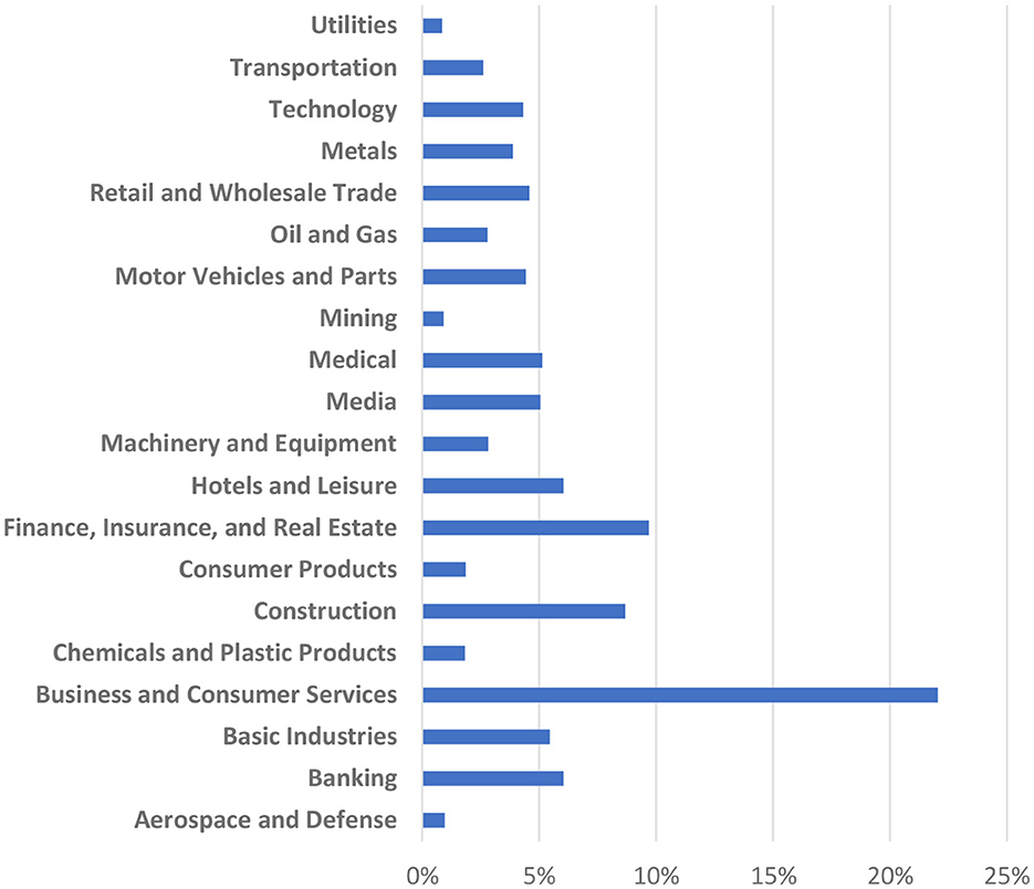
Figure 7. Industry composition of 2050 expected losses in no-climate-effects baseline. Source: NGFS and Z-risk engine.

4.2. Future research needs to seek a statistical calibration, add industry and region effects, and TTC effects

These estimates rely on hypothetical climate-change multipliers, not yet estimated empirically. In future research, analysts will want to explore calibrating the climate/credit volatility relationship. To obtain credible estimates of the effect of climate change on credit losses, one hopes for a formulation that is both theoretically plausible and has been found to be potentially statistically reliable.

Additionally, the above results come from a model with proportionately the same climate-change effects on volatility in every industry and region. Future work might introduce varying effects, with more climate-sensitive industries and regions having higher climate-volatility multipliers. Finally, future climate stress testing that applies multi credit-factor models can also allow or changing TTC risk attributes.

5. ZRE measures and models used in this study

This section describes the credit-cycle measures and models used in this study. All three models produce loss estimates for a hypothetical, dynamic portfolio with attributes that imply long-run loss rates similar to those experienced by US bank, C&I loans. As a common convention for mimicking a dynamic portfolio, the through-the-cycle (TTC) attributes of the hypothetical portfolio remain fixed over time. Then, in each future quarter, the models draw on the industry-region, simulated Zs in converting the TTC attributes to PIT ones and in estimating PIT PDs, LGDs, EADs, and credit losses.

5.1. Industry and region Z indices

ZRE's industry and region Zs derive from point-in-time (PIT) PDs estimated for a comprehensive set of listed companies across the world. In this study, we use Moody's CreditEdge EDFs (Nazeran and Dywer, 2015; Moody's Analytics, 2016) as the source of the listed-company PDs. We obtain the industry and region Zs by

• transforming the monthly, listed-company EDFs into default-distance (DD) measures by applying the negative of the inverse-normal function (DD = −Θ⁽⁻¹⁾ (EDF)),

• summarizing those DDs for selected, industries and regional grouping by taking medians,

• detrending the monthly median, DD series,

• forming DDGAPs for each industry and region by expressing the detrended, monthly median DDs as deviations from long-run means, and

• dividing the DDGAPs for each industry or region by the standard deviation of annual changes in those DDGAPs.

In most ZRE applications, the industry and region, Z indices get combined to form industry-region ones, which in turn enter as inputs into the PD, LGD, and EAD models. The combinations are weighted averages, with the weights set so as to best explain the past, quarterly changes in listed-company, DDs. We see below in the case of North America that the industry-region Zs have common cyclical fluctuations and some sector specific ones (Figure 8).

FIGURE 8

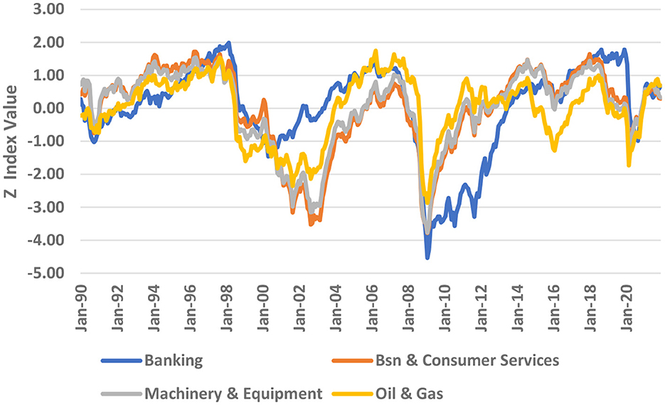
Figure 8. Historical values of selected North American industry Zs. Source: Z-risk engine.

5.2. MM models for the stochastic evolution of Zs

ZRE applies mean-reversion-momentum (MM) models in generating quarterly, Z sims. The MM models involve formulas of the kind below.

$\begin{array}{ll}\Delta Z_{(q+1)}^S=m_1^S{Z}_q^S+m_2^S\Delta Z_q^S+{\epsilon }_{(q+1)}^S& (1)\end{array}$

In (1) q denotes an integer index identifying quarters, $\Delta Z_q^S$ the change in the Z for segment S from quarter-end q−1 to quarter-end $q,m_1^S$ the quarterly mean-reversion coefficient for segment $S,m_2^S$ the quarterly momentum coefficient for that segment, and ${\epsilon }_{q+1}^S$ the unexpected shock (or innovation) to $\Delta Z_{q+1}^S$. In the IRMC model S identifies various, industries and regions, whereas in the SFMC model, S identifies the different, MEV Zs.

In this study, the shocks driving the Z sims have volatilities that rise as the climate warms as measured by the GMT. Thus, under more severe climate scenarios, the sims include more disparate Z values implying greater downturns and higher credit losses.

5.3. IRMC model overview

The IRMC model runs Monte Carlo, industry and region, Z sims that ultimately lead to credit-loss sims. In producing a credit-loss sim, ZRE-IRMC:

• draws jointly, from a multivariate-normal or historical-empirical distribution, a quarterly series of Z shocks for each industry and region,

• enters those Z shocks into the related, MM models and, by solving iteratively starting from an initial quarter with known Z and Z values, simulates future, industry and region Zs,

• combines the simulated, industry and region Zs for each permissible, industry-region pair and obtains the related, quarterly, industry-region Zs,

• enters the industry-region Zs into PD, LGD, and EAD models for the facilities in a corporate and commercial portfolio and thereby produces a quarterly sim for defaults and credit losses.

For each climate scenario, we've run 1,000 sims extending 114 quarters staring in 2022Q3 and ending at 2050Q4. The IRMC sims in this study involve random selection of historical shocks.

5.4. SFM model overview

The SFM runs d scenarios conditional on assumed MEV paths, including those used in implementing the regulatory scenarios. The SFM:

• draws on predetermined, MEV paths,

• converts those MEV paths into paths for stationary, credit-cycle measures denoted MEV Zs,

• applies a bridge model in determining the industry and region, Z paths implied by the MEV-Z ones,

• combines the industry and region Zs into composite, industry-region Zs,

• enters the industry-region Zs into the PD, LGD, and EAD models for the facilities in the representative, C&I portfolio and thereby estimates the related, credit losses.

5.5. SFMC model overview

The SFMC model used in this study appends a Monte Carlo engine to the SFM. This involves MM models for simulating MEV Zs. The SFMC sims jointly select shocks for both the Macro-Z MM models and the bridge models. In running the sims, SFMC

• draws at random, for each projection quarter, a row of values from a table of historical, calendar-quarter, Macro-Z and bridge-model residuals,

• enters into each MEV-Z, MM model the selected residual, known values of $Z_q^M$ and $\Delta Z_q^M$, and solves for $\Delta Z_{(q+1)}^M$ and $Z_{(q+1)}^M,$

• puts, into each bridge-model equation, the selected, industry or region, bridge-model residual, the $Z_q^S$, $\Delta Z_q^S$ values, and, for all MEV-Z variables, the $\Delta Z_{(q+1)}^M$, and $\Delta Z_q^M$ values, and solves for $\Delta Z_{(q+1)}^S$ and $Z_{(q+1)}^S$,

• combines the industry and region Zs for each valid IR pair and derives the industry-region Zs, and places the related, industry-region Zs into the PD, LGD, and EAD models for each facility classified within each industry-region sector and solves for the related losses.

5.6. MEV Zs used in this study

The SFMC model applied in this paper includes MEV Zs that derive, respectively, from the Wilshire 5000 stock-price index, US GDP, and Baa spreads. We explain the derivations next.

ZRE translates a stock-price index to a stock-price Z (ZE) by

• forming ratios of the quarterly, stock-price index to autoregressive-first-order (AR(I)), moving averages of that index;

• calculating natural logarithms of the ratios; and vexpressing the logarithmic ratios as deviations from the mean value with that result in turn divided by the standard deviation of annual changes in the logarithmic ratios.

ZRE converts a GDP series to a GDP Z (ZG) in the same way by

• forming ratios of quarterly GDP to AR(1) moving averages of quarterly GDP;

• calculating natural logarithms of those ratios; and

• expressing the logarithmic ratios as deviations from the long-run, average value with that result in turn divided by the standard deviation of annual changes in the logarithmic ratios.

ZRE converts Baa spreads to spread-Z indices (ZS) by

• dividing by 0.6, representing the conventional, risk-neutral, LGD for corporate bonds, and obtaining imputed PDs,

• applying the negative of the inverse-normal function to the imputed PDs and thereby deriving estimated DDs,

• subtracting the 1990-to-date average value of the DDs and dividing by the standard deviation of 1990-to-date, annual changes in the DDs.

5.7. Bridge model

For this study, we've estimated the bridge models using pooled, least-squares regression of one-quarter changes in the Zs for each of 21 industry and the two, North American, regional groupings on (1) one-quarter lagged values of those Zs; (2) one quarter lagged values of one-quarter changes in those Zs; and (3) current and one-quarter-lagged values of quarterly changes in the ZE, ZS, and ZG, MEV-Z indexes (Table 3). The estimation uses data from 1990Q3 to 2022Q1. The bridge model for the CCAR scenarios and SFMC sims include three, MEV Zs. Due to the NGFS scenarios including values only for GDP and not stock prices and credit spreads, the bridge model used in those cases includes only one, MEV Z (GDP Z).

TABLE 3

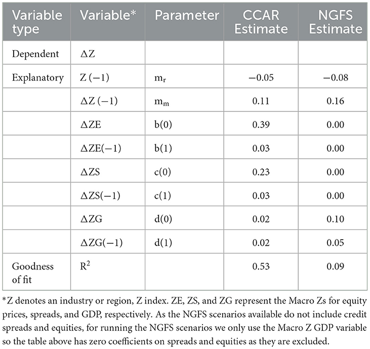
Table 3. US bridge model variables and coefficients.

5.8. Estimating scenario losses for facilities in the hypothetical portfolio

The quarterly, industry-region Zs enter into facility PD, LGD, and EAD models and thereby produce quarterly estimates of losses. See below for more detail.

5.8.1. Facility PDs

In each scenario in each quarter for each facility in the representative portfolio, we apply a Probit PD model in deriving a quarterly PD. A Probit model uses a standard-normal, cumulative distribution function (CDF) in transforming a DD measure into a PD. As applied here, th e model has the following inputs: the quarterly, TTC PD transformed into a DD; the industry-region Z expressed relative to a normal Z consistent with the TTC PD; and various volatility parameters that convert the Z factor into a DD variation scaled for a quarterly model. The Z factor input together with the volatility parameters convert the TTC PD into a PIT one.

5.8.2. Facility LGDs

The facility LGDs arise from a Tobit LGD model. This model has point masses at 0% and 100% and uses a normal CDF for the frequency of LGD outcomes above 0% and below 100%. In this study, the model has the following, facility inputs: TTC LGD; and the relevant, industry-region Z. The parameters of the model come from past, empirical results. We solve for the expected value of LGD, conditional on the scenario Z.

5.8.3. Facility EADs

We use a CCF model sensitive to the credit cycle in deriving EADs for each facility in each scenario quarter. In such a model, the utilization in default rises above the performing facility's expected utilization rate by a proportion (CCF) of the fraction unutilized under non-default conditions. The CCF in this study comes from a Probit model with the relevant, industry-region Z as an input. We scale the model so that, if Z is zero, the CCF equals the TTC value that appears as an attribute in the portfolio file. We've set the Z sensitivity of CCFs to that estimated in past empirical work.

Each facility's expected credit loss (ECL) in a scenario quarter derives as a product of the facility's, PD, expected LGD (ELGD) and expected EAD (EEAD) values for that quarter. The ECL and all of the component, expected values are conditional on the Z value in the quarter. We obtain the ECL for the C&I portfolio or various, sub-portfolios by summing the constituent, facility ECLs.

5.9. Attributes of the representative, C&I portfolio

The hypothetical, C&I portfolio includes a broad set of industries roughly representative of all, C&I loans (Table 4). Each industry-region Z index arise as a weighted average of a global industry, Z index and a regional, Z index. In the case of non-financial industries, the regional index in the combination includes only non-financial companies in its construction. In the case of financial industries, the regional index in the combination includes only financial companies. The weights involved in forming industry-region indexes derive from regressions of quarterly changes in DDs of listed companies within each industry on quarterly changes in the associated, industry and region, median DDs. Note that ZRE also creates an agriculture industry, but, in the Fed/OCC loan-loss data, agricultural loans are in a separate category outside of C&I. Thus, in this study, we exclude agricultural as a relevant industry.

TABLE 4

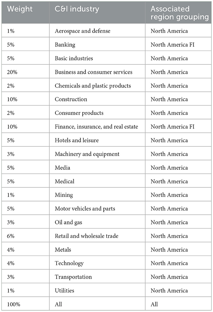
Table 4. Industry composition of the representative C&I portfolio.

The portfolio in the scenarios includes a mixture of revolving (RCF) and term loan (TL) facilities with TTC attributes that remain fixed over time (Table 5). This practice of holding the TTC attributes constant represents a tractable way of running dynamic portfolio simulation under the assumption of a fixed, risk appetite. To simplify the model, we assume that the attributes are the same for every industry-region segment.

TABLE 5

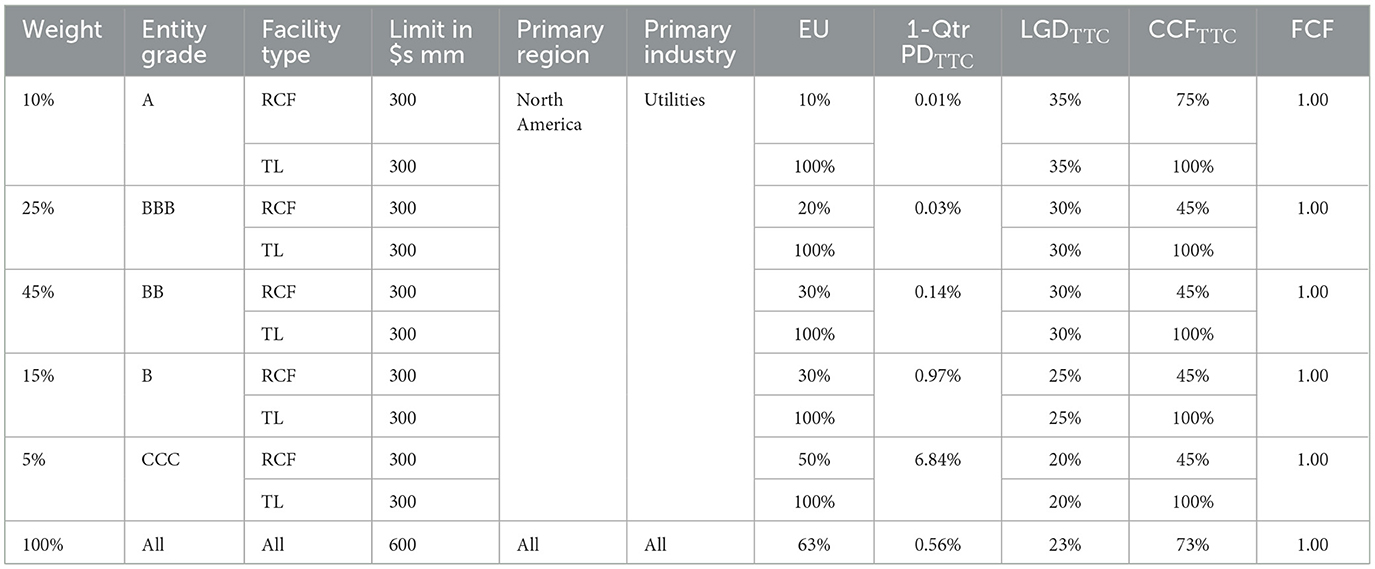
Table 5. Industry composition of the representative C&I portfolio.

5.10. Background on validation of the ZRE approach

The validation of ZRE comes from empirical studies in which we find that:

• adding ZRE's industry-region Zs to PD and LGD models drawing on financial ratios and judgmental scores increases the goodness-of-fit by a statistically significant, order of magnitude (Table 6),

• applying ZRE in back tests involving a representative, C&I, loan portfolio, we get estimates that align closely with actual C&I losses (Figure 9), and

• replacing the longstanding random-walk models with ZRE's mean-reversion-momentum ones, we get statistically significantly better estimates of Z indices.

TABLE 6

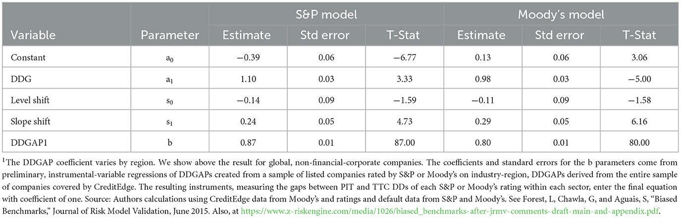
Table 6. Estimates of PIT-PD models for S&P-rated and Moody's-rated, non-financial companies.

FIGURE 9

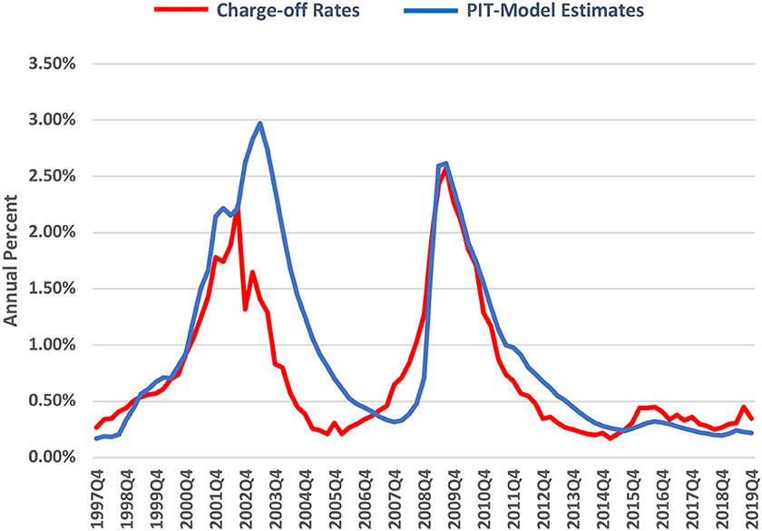
Figure 9. Back test over 1997Q4-2018Q4 for a C&I- loan portfolio.

6. Summary

In this paper we have extended the climate stress test literature by presenting three different assessments of future credit risk losses potentially related to climate change. The assessments utilize the well-known NGFS scenario climate stress test approach in conjunction with an empirical credit-factor portfolio model. We also apply a non-empirical, illustrative NGFS GMT-to-volatility approach to assess the potential impacts of future aggregate climate shocks and volatility. We also use these assessments to highlight some of the recent industry discussion points related to the complexity surrounding developing climate stress tests generally.

The familiar NGFS climate-change scenarios show global warming as slowing economic growth rates, but not increasing the amplitude of economic cycles. As a result, climate change assessments undertaken to-date have suggested quite limited effects on future long-run credit losses. This paper assumes, in contrast, that climate change increases the volatility of credit shocks which have historically been a key contributor to cyclical credit losses. This general assumption in these three assessments resembles the presumption that climate change leads to more extreme weather, leading to higher future physical risk impacts and the potential for additional complex social and other cascading (tipping point) economic impacts. Not surprising, with climate change raising the volatility of credit factors, we find that credit losses increase as global warming continues. Moreover, the largest impact occurs in severe recession scenarios.

While the focus here is on aggregate shocks and volatility, there are natural extensions to the research presented that include: (1) calibrating an empirical relationship between climate change and volatility, (2) applying differential volatilities to specific industry sectors and regions, and, (3) allowing for industry TTC risk parameters to vary.

Author's note

This paper summarizes three Z-Risk Engine Draft Working Papers published at the 2022 RiskMinds International Conference in Barcelona, in November 2022 (Aguais and Forest, 2022a,b,c). All errors and omissions remain the responsibility of the authors.

Data availability statement

The original contributions presented in the study are included in the article/supplementary material, further inquiries can be directed to the corresponding authors.

Author contributions

Both authors listed have made a substantial, direct, and intellectual contribution to the work and approved it for publication.

Conflict of interest

SA and LF were employed by Aguais and Associates, LTD.

Publisher's note

All claims expressed in this article are solely those of the authors and do not necessarily represent those of their affiliated organizations, or those of the publisher, the editors and the reviewers. Any product that may be evaluated in this article, or claim that may be made by its manufacturer, is not guaranteed or endorsed by the publisher.

Footnotes

1. ^The foundation of the Z-Risk Engine approach using a systematic credit-factor approach, “Z,” was first outlined in Belkin et al. (1998a,b).

2. ^For clarity, the time horizon for CCAR scenarios is “short-run” and the NGFS scenarios are usually applied to longer-run horizons. The comparison we make focuses on the effects of systematic factors on credit risk not the time horizon differences.

3. ^The “Z” notation is used throughout the paper to denote systematic variables. These include systematic variables derived from MEVs and are also applied to industry sectors and geographic regions.

4. ^As we discuss in more detail below, we use an illustrative GMT-to-Volatility approach because of the lack of statistically identifiable climate impacts on credit factor models generally.

5. ^There is an entire literature discussing the pros and cons of using IAM-style models to drive CST approaches, which we exclude from this brief discussion of industry concerns, see Monasterolo et al. (2022) for a more detailed discussion of IAM-style models generally.

6. ^CST approaches like the one under development at the ECB, complement the top-down NGFS scenarios with disaggregated variables linked to a large sample of European-wide commercial firms including geo-location data to assess firm-level credit risks. However, this approach is still primarily driven top-down.

7. ^Concerns with more “top–down” model approaches not successfully capturing lower-level, sectoral variation is also just as relevant for projecting expected credit losses under the IFRS9 or CEC accounting rules. Nearly all banks currently use a combination of their IRB credit models regressed on macro-economic variables (MEV). Using just MEVs in general to predict systematic changes in credit risk for IFRS9 does not fully capture the PIT credit risk variability observed at the industry sector and region level during the last 3 recessions.

8. ^Kemp et al. (2022), p. 1.

9. ^Adding climate narratives given substantial uncertainty is a positive suggestion and seems to stem directly from frustration with the use of “stylized” NGFS scenarios. We agree with these points but also suggest a more solid objective and statistical foundation for assessing systematic climate risk, as presented in these papers is also a key part of a more “holistic” CST framework.

10. ^See the DBS Bank Case Study for a review how a ZRE implementation supports both stress testing and IFRS9 (Z-Risk Engine Case Study, 2022).

11. ^Dornbusch's Law is usually ascribed to “overshooting” or excess volatility in foreign exchange markets but is applied here as well to credit risk. See Dornbusch (1976).

References

Adenot, T., Briere, M., Counathe, P., Jouanneau, M., Le Berthe, T., and Le Guenedal, T. (2022). Cascading Effects of Carbon Price Through the Value Chain: Impact on Firms' Valuation', Amundi Working Paper 125-2022. Available online at: https://research-center.amundi.com/article/cascading-effects-carbon-price-through-value-chain-impact-firm-s-valuation

Google Scholar

Aguais, S. (2022). “Musings on long run climate stress test modelling for banks,” in Presentation, Marcus Evans, Climate Stress Testing. Available online at: www.z-riskengine.com (accessed June 16, 2022).

Aguais, S., and Forest, L. (2022a). Climate Change Credit Risk Triptych, Paper One: Smooth NGFS Climate Scenarios Imply Minimal Impacts on Corporate Credit Losses. Available online at: www.z-riskengine.com

Google Scholar

Aguais, S., and Forest, L. (2022b). Climate Change Credit Risk Triptych Paper Two: Climate Change Volatility Effects Imply Higher Credit Losses. Available online at: www.z-riskengine.com

Google Scholar

Aguais, S., and Forest, L. (2022c). Climate Change Credit Risk Triptych Paper Three: Climate Change Macro Volatility Effects Imply Higher Credit Losses. Available online at: www.z-riskengine.com

Google Scholar

Allen, T., Dees, S., Caicedo Graciano, C. M., Chouard, V., Clerc, L., de Gaye, A., et al. (2020). Climate-Related Scenarios for Financial Stability Assessment: An Application to France (July 16, 2020). Banque de France Working Paper No. 774. Available online at: https://ssrn.com/abstract=3653131

Google Scholar

Alogoskoufis, S., Dunz, N., Emambakhsh, T., Hennig, T., Kaijser, M., Kouratzoglou, C., et al. (2021). “ECB, economy-wide climate stress test, methodology and results,” in Proceedings of the 2021, European Central Bank, Occasional Paper Series Number 281, September.

Google Scholar

Baldassarri Höger von Högersthal, G., Lui, A., Tomičić, H., and Vidovic, L. (2020). Carbon pricing paths to a greener future, and potential roadblocks to public companies' creditworthiness. J. Energy Mark. 13, 24. doi: 10.21314/JEM.2020.205

CrossRef Full Text | Google Scholar

Battiston, S., Mandel, A., and Monasterolo, I. (2019). CLIMAFIN Handbook: Pricing Forward-Looking Climate Risks Under Uncertainty. Available online at: https://papers.ssrn.com/sol3/papers.cfm?abstract_id=3476586

Google Scholar

Battiston, S., Mandel, A., Monasterolo, I., Schütze, F., and Visentin, G. (2017). A climate stress-test of the financial system. Nat. Clim. Change 7, 283–288. doi: 10.1038/nclimate3255

CrossRef Full Text | Google Scholar

Belkin, B., Suchower, S., and Forest, L. (1998a). A one parameter representation of credit risk and transition matrices. Credit-Metr. Monit. 1, 45–56.

Google Scholar

Belkin, B., Suchower, S., and Forest, L. (1998b). The effect of systematic credit risk on loan portfolios and loan pricing. Credit-Metr. Monit. 13, 17–28.

Board of Governors of the Federal Reserve System (2022a). Charge-Off and Delinquency Rates on Loans and Leases at Commercial Banks. Washington, DC: Board of Governors of the Federal Reserve System. Available online at: https://www.federalreserve.gov/releases/chargeoff/chgallsa.htm

Google Scholar

Board of Governors of the Federal Reserve System (2022b). Stress Tests and Capital Planning. Washington, DC: Board of Governors of the Federal Reserve System. Available online at: https://www.federalreserve.gov/supervisionreg/ccar.htm

Google Scholar

Boirard, A., Payerols, C., Overton, G., De Albergaria, S. S., and Vernet, L. (2022). Climate scenario analysis to assess financial risks: some encouraging first steps. Bull. Finan. Stabil. Finan. Syst. 48, 241. Available online at: https://publications.banque-france.fr/en/climate-scenario-analysis-assess-financial-risks-some-encouraging-first-steps

Google Scholar

Bouchet, V., and Guenedal, L. (2020). Credit Risk Sensitivity to Carbon Price. Amundi Working Papers, 95–2019. Available online at: https://research-center.amundi.com/article/credit-risk-sensitivity-carbon-price

Google Scholar

Capasso, G., Gianfrate, G., and Spinelli, M. (2020). Climate change and credit risk. J. Clean. Prod. 266, 121634. doi: 10.1016/j.jclepro.2020.121634

CrossRef Full Text | Google Scholar

Chawla, G., Forest, L., and Aguais, S. (2016). Point-in-time loss-given default rates and exposures at default models for IFRS 9/CECL and stress testing. J. Risk Manag. Finan. Institut. 9, 249–263.

Google Scholar

Cliffe, M. (2021). Climate Shock: Time for More Stressful Tests on Banks. Available online at: https://markcliffe.wordpress.com/2021/10/30/climate-shock-time-for-more-stressful-tests-on-banks/

Google Scholar

Cliffe, M. (2022). Real World Climate Scenarios (RWCS) Roundtable, Held on May 4, 2022, Notes Available on LinkedIn.

Cliffe, M., Verdagaal, W., and Clark, M. (2022). Real World Climate Scenarios (RWCS) Roundtable. Available online at: https://raoglobal.org/blog/real-world-climate-scenarios-rwcs-roundtable

Google Scholar

Dornbusch, R. (1976). Expectations and exchange rate dynamics. J. Polit. Econ,. 84, 1161–1176.

Google Scholar

ECB/ESRB and Project Team on Climate Risk Monitoring (2021). Climate-Related Risk and Financial Stability. Frankfurt am Main: European Systematic Risk Board.

Forest, L., and Aguais, S. (2019a). Variance Compression Bias in Expected Credit Loss Estimates Derived From Stress-Test Macroeconomic Scenarios. Z-Risk Engine Working Paper. Available online at: https://www.z-riskengine.com/media/g34nb3i3/variance-compression-bias-in-expected-credit-loss-estimates.pdf

Google Scholar

Forest, L., and Aguais, S. (2019b). Scenario Models Without Point-in-Time, Market-Value Drivers Understate Cyclical Variations in Wholesale/Commercial Credit Losses. Z-Risk Working Paper. Available online at: https://www.z-riskengine.com/media/q3gkiqrd/zre_stress_understatement_using_gdp_drivers.pdf

Google Scholar

Forest, L., and Aguais, S. (2019c). Inaccuracies Caused by Hybrid Credit Models and Remedies as Implemented by ZRE. Z-Risk Working Paper. Available online at: https://www.z-riskengine.com/media/y5tj421m/zre_inaccuracies-caused-by-hybrid-credit-factors_sep19.pdf

Google Scholar

Garnier, J., Gaudemet, J.-P., and Gruz, A. (2022). The Climate Extended Risk Model (CERM). arXiv [Preprint]. arXiv: 2103.03275. Available online at: http://arxiv.org/2103.03275.pdf

Google Scholar

Hughes, T. (2021a). The Futility of Stress Testing for Unprecedented Scenarios. Available online at: https://www.garp.org/risk-intelligence/operational/the-futility-of-stress-testing-for-unprecedented-scenarios

Google Scholar

Hughes, T. (2021b). The Case for Monte Carlo Simulations. Available online at: https://riskweighted.com/2021/09/21/the-case-for-monte-carlo-simulations

Google Scholar

Hughes, T. (2022). Scenario Analysis, Assessing the Quality of the Journey. Available online at: https://www.garp.org/risk-intelligence/operational/accessing-quality-journey-220729

Google Scholar

Kemp, L., Xu, C., Depledge, J., Ebi, K. L., Gibbins, G., Kohler, T. A., et al. (2022). Climate endgame: exploring catastrophic climate change scenarios. Proceed. Natl. Acad. Sci. 119, e2108146119. doi: 10.1073/pnas.2108146119

PubMed Abstract | CrossRef Full Text | Google Scholar

Khanna, P. (2022). What comes after the coming climate anarchy? Ideas Clim. Change 15, e10034.

Google Scholar

McKay, A. (2021). Don't look up, paramount pictures. Film Quart. 75, 5–11.

Google Scholar

Monasterolo, I., Nieto, M., and Schets, E. (2022). “The good, the bad and the hot house world: conceptual underpinnings of the NGFS scenarios and suggestions for improvement,” in Working Paper Presented Scenarios Forum. doi: 10.2139/ssrn.4211384

CrossRef Full Text | Google Scholar

Moody's Analytics (2016). CreditEdge: A Powerful Approach to Measuring Credit Risk, Brochure. Washington, DC: Moody's Analytics. Available online at: https://www.moodysanalytics.com/-/media/products/CreditEdge-Brochure.pdf

Google Scholar

NASA (2020). Global Climate Change. Washington, DC: NASA. Available online at: https://climate.nasa.gov/vital-signs/global-temperature/

Google Scholar

Nazeran, P., and Dywer, D. (2015). Modelling Methodology: Credit Risk Modelling of Public Firms: EDF9. Washington, DC: Moody's Analytics.

Google Scholar

NGFS. (2022a). Climate Scenarios Database: Technical Documentation. Available online at: https://www.ngfs.net/sites/default/files/media/2022/11/21/technical_documentation_ngfs_scenarios_phase_3.pdf

Google Scholar

NGFS. (2022b). NGFS Scenarios for Central Banks and Supervisors. Available online at: https://www.ngfs.net/sites/default/files/medias/documents/ngfs_climate_scenarios_for_central_banks_and_supervisors_.pdf

Google Scholar

Pitman, A. J., Fiedler, T., Ranger, N., Jakob, C., Ridder, N. N., Perkins-Kirkpatrick, S. E., et al. (2022). Acute climate risks in the financial system: examining the utility of climate model projections. Environ. Clim. Res. 1, 25002. doi: 10.1088/2752-5295/ac856f

CrossRef Full Text | Google Scholar

Stern, N., Stiglitz, J., and Taylor, C. (2022). The economics of immense risk, urgent action and radical change towards new approaches to the economics of climate change. J. Econ. Methodol. 29, 181–216. doi: 10.1080/1350178X.2022.2040740

CrossRef Full Text | Google Scholar

Vermeulen, R., Schets, E., Lohuis, M., Kölbl, B., Jansen, D. J., and Heeringa, W. (2021). The heat is on: a framework for measuring financial stress under disruptive transition scenarios. Ecol. Econ. 190, 107205. doi: 10.1016/j.ecolecon.2021.107205

CrossRef Full Text | Google Scholar

Wagner, G., and Weitzman, M. (2015). Climate Shock the Economic Consequences of a Hotter Planet. Princeton: Princeton University Press. doi: 10.1515/9781400865475

CrossRef Full Text | Google Scholar

Wallace-Wells, D. (2019). The Uninhabitable Earth. London: Penguin Random House. doi: 10.7312/asme18999-010

CrossRef Full Text | Google Scholar

Z-Risk Engine Case Study (2022). Supporting Integrated IFRS 9 and Stress Testing at DBS Bank. Washington, DC: Z-Risk Engine Case Study. Available online at: www.z-riskengine.com

Google Scholar