Trends and variability of total column ozone in the Third Pole

Highlights

- Highest mean TCO over the northern and lowest over the southern Third Pole.

- South of Third Pole has about 20% less TCO compared to that in the north.

- A decreasing trend in TCO over Third Pole is observed, about −0.45 DU/year.

- TCO variability is mostly driven by tropopause height and atmospheric dynamics.

1. Introduction

Atmospheric ozone (O₃) is an active trace gas, produced naturally both in the troposphere and stratosphere. In the troposphere, O₃ is a pollutant with detrimental impact on human health and ecosystem. In addition, it is a good oxidant and a greenhouse gas (GHG) with positive feedback to surface temperature (Zeng et al., 2008; Xu et al., 2016). However, it absorbs harmful solar ultraviolet (UV) radiation in the stratosphere and protects life on the earth. Therefore, as an important GHG and UV radiation absorber, O₃ has a great role in atmospheric radiation balance and climate change (Forster and Shine, 1997; IPCC, 2013). Due to the impact of human activities, the global total column ozone (TCO) has decreased over the past few decades, particularly in the polar and midlatitude regions (WMO (World Meteorological Organization), 2018). However, because of the implementation of Montreal Protocol and its amendments and adjustments (MPA), the signature of O₃ recovery has been found in the high and mid-latitudes (Chipperfield et al., 2015; Nair et al., 2015; Solomon et al., 2016; de Laat et al., 2017; Kuttippurath and Nair, 2017; Kuttippurath et al., 2018; Pazmiño et al., 2018; Weber et al., 2018). Past studies show that the recovery of stratospheric ozone is not uniform in all latitudes (WMO (World Meteorological Organization), 2018), and there are still uncertainities in the direction and magnitude of these trends in the lower latitudes. In the context of global ozone recovery and climate change, whether TCO trends in TP would be similar to those over the other regions in the same latitude band is an interesting topic of further investigation.

The Hindu Kush Himalaya (HKH) and Tien Shan mountains within the region 10°-45° N and 60°-105° E are called the Third Pole (TP) of Earth (Qiu, 2008; Wester et al., 2019). The region is widely known because of its high mountaneous topography, highest plateau and home to the largest reserve of fresh ice mass on the planet outside the poles (Yao et al., 2012). Past studies show that TP receives substantial amount of air pollutants within and from the adjacent boundary regions, including Indo-Gangatic Plain (IGP) (Bonasoni et al., 2012; Cong et al., 2015), east China (Lin, 2012) and other parts of Asia (Wester et al., 2019). These pollutants are deleterious to human health, and minacious to food security, water resources and regional climate by influencing the incoming solar radiation, and alter the albedo of snow and ice surfaces (Kang et al., 2019). Environmental condition in some regions of TP has been continuously deteriorating for the past few decades (Gautam et al., 2003). Therefore, it is essential to continuously monitor O₃ in TP for change detection and to take mitigation measures in the context of climate change.

There are only limited number of measurement stations in TP because of its complex topography and inaccessibility. Therefore, it is difficult to obtain continuous and accurate data for O₃ from ground-based measurements. On the other hand, satellite measurements provide continuous global measurements. Studies suggest that TCO over Tibetan Plateau (TBP) is very low as compared to the non-TBP regions in the same latitude band (Zou, 1996; Zhou et al., 2006). Factors such as high altitude topography, climate change and anthropogenic activities are mainly responsible for this (Zhang et al., 2014). Tian et al. (2008) suggest that high altitude topography and seasonal variability in the tropopause height are the major factors casusing the low TCO over TP.

There are several studies related to ozone trends in TBP, but not for the complete TP region as analyzed in this study. For instance, Zou (1996) estimated a negative TCO trend (−0.79 ± 0.82 DU/yr) over TBP for the period 1979–1991. Zhou and Zhang (2005) found a significant decline (−3%/dec in February) in Total Ozone Mapping Spectrometer (TOMS) TCO over TBP in spring and summer during the period 1979–2002. Zhou et al. (2013) showed a substantial decrease in TCO (−0.4 DU/yr) over TBP from 1979 to 2010 as analyzed using the TOMS/Solar Backscatter Ultraviolet (SBUV) satellite data in winter and spring. They also reported a strong correlation between TCO and lower stratospheric temperature there. Zhang et al. (2014) pointed out that the TCO in the Total Ozone Low (TOL) region over TP in winter is decreasing at a rate of 1.4 DU/dec, although TCO over TBP started to recover since the mid-1990s, as shown in their analysis. This decreasing trend in ozone at the TOL region would likely to slowdown the recovery of TCO in TBP. Similarly, Zou et al. (2020) observed a substantial decrease (−0.83 DU/yr) and increase (0.02 DU/yr) in the 30° N−35° N region, in the Solar Backscatter Ultraviolet (SBUV) TCO data during the periods 1979–1996 and 1997–2018, respectively.

As the trends estimated in different regions of TP have different values and do not cover the entire TP (most studies are for the TBP areas), we focus on the spatiotemporal variability of TCO in TP for the period 2005–2020 by using a combined Ozone Monitoring Instrument (OMI) and Global Ozone Monitoring Experiment (GOME)-2B data. Furthermore, we also examine the TCO changes in 20 selected cities in and around TP. The cities include Kabul, Peshawar, Kuzdan, Srinagar, Deharadun, Shilong, Silchar, Agartala, Thimphu, Kathmandu, Chittagong, Naypyitaw, Xinning, Lhasa, Kunming, Uramqi, Dushanbe, Almaty, Tashkent and Bishkek from 12 countries, including Afghanistan, Pakistan, India, Bhutan, Nepal, Bangladesh, Myanmar, China, Kazakhstan, Kyrgyzstan, Uzbekistan and Tajikistan and they cover the entire TP and its boundary regions. This study would help to understand the environmental changes in TP in the context of climate change.

2. Materials and methods

The study area covers the entire TP region, i.e., 10°-45° N and 60°-105° E, as illustrated in Figure 1. We use a combined dataset made by using the measurements of OMI from January 2005 to December 2014 and GOME-2B from May 2013 to December 2020. OMI has the advantage of daily global coverage with high spatial resolution and GOME-2B has an additional advantage of a stronger anthropogenic signal due to its relatively early overpass in daytime. OMI on Aura satellite was launched in 2004 (Levelt et al., 2006), which operates under the nadir mode and measures the backscattered radiances in three different channels ranging from 270 to 500 nm with a resolution of 0.42–0.63 nm (Schoeberl et al., 2006). The instrument has a wide field of view of 114° with a cross-track swath of 2,600 km, and daily global coverage with a spatial resolution of 13 km × 24/48 km (along × cross-track) (Eskes et al., 2003; Levelt et al., 2006). As it measures the entire ozone absorption band, TCO is derived by using the differential optical absorption spectroscopy (DOAS) method (Veefkind et al., 2006). The OMI column ozone shows good agreement with other independent measurements, within 5–10% (Kroon et al., 2008).

FIGURE 1

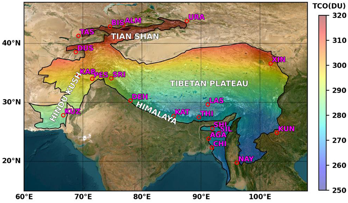
Figure 1. Third Pole and the adjacent cities in the region. The annual mean TCO (DU) averaged over the period 2005–2020 is shown. The city name, latitude, longitude, and elevation are given in Table 1.

TABLE 1

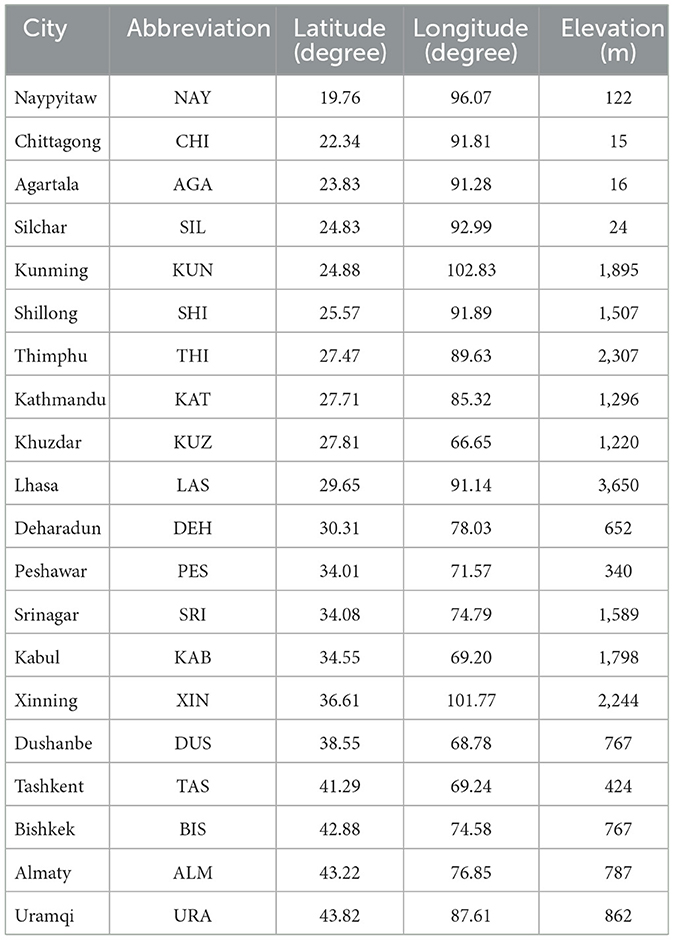
Table 1. The coordinates and elevation of 20 major cities in and around the study area.

GOME-2B is the continuation of previous missions employed for long-term monitoring of atmospheric trace gases, which started with GOME on the MetOp satellite. GOME-2B was launched on European Space Agency MetOp-A satellite in 2006 (Callies et al., 2003). All MetOp satellites (i.e., MetOp-A, MetOp-B, and MetOp-C) are now in operation in the same orbit, but separated by 48.93 min. GOME-2B is also a nadir-viewing, UV Visible scanning spectrometer with four bands in the 240–790 nm range. It has a ground pixel size of 80 × 40 km² and a scan-width of 1,920 km, which provide a daily global coverage in the same spectral range as for GOME (Loyola et al., 2011).

Satellite-based TCO observations are available from different missions since the 1970s. The cross-mission sensors provide continuous TCO observations. However, the cross-mission biases are always associated with multiple sensors in common time-space domain depending on satellites, instruments, calibration techniques and retrieval algorithms. Accurate data merging procedure is required to make long-term data for change detection and attribution of trends. Kuttippurath et al. (2013) reported that even a small drift between two different TCO time series could result in apparent changes in ozone recovery trends. Henceforth, cross-mission bias correction is important for making a long-term data.

Here, we merge the OMI (January 2005–December 2014) and GOME-2B (May 2013–December 2020) data using the modified bias correction method described by Bai et al. (2016), where a percentile with respect to a given data value in the observation prior to the overlap period is determined using the nearest or the same value in the overlap period. This percentile is then used to determine the value of TCO from the new instrument. The difference in TCO during the overlap period to the previous measurements is the raw bias associated with the instrument. The raw bias is then used to estimate the cross mission bias and this bias is added to the previous measurements to make a robust long-term dataset. Here, the TCO observations from OMI are then projected to GOME-2B level since GOME-2B is the recently launched satellite with better instrumentation. The advantage of modified bias correction method compared to other statistical bias correction methods is the use of median values to avoid the uncertainties due to outliers. In addition, this method does not depend on the raw observations, but on the distribution mapping of control observations during the overlap period, which is more adaptive and is able to handle observations at different time scales. We applied this procedure to make a long-term continuous data from 2005 to 2020 to analyze the spatial and temporal changes of TCO in TP. The observations during the overlapping period of both satellites (May 2013–December 2014) are shown in Supplementary Figure S1. The GOME-2B measurements show relatively higher ozone than that of OMI over the entire TP, though the spatial distribution of TCO is consistent in both datasets, and the differences are within 5–10 DU. The difference is comparatively larger (10 DU) in the regions north of 30° N (Supplementary Figure S1, bottom).

We have also employed a multi-linear regression (MLR) model to find the trends and contribution of different processes to the ozone changes in TP (e.g., Kuttippurath et al., 2013). The predictors include the Brewer-Dobson Circulation (BDC) represented by Eddy Heat Flux (EHF) at 100 hPa calculated using the ERA5 (the fifth generation of European Centre for Medium-Range Weather Forecasts reanalysis) data, El Niño-Southern Oscillation (ENSO) index and Solar Flux (SF) at 10.7 cm wavelength. In addition, the regression procedure also considers the two orthogonal components of Quasi Biennial Oscillation (QBO), QBO_a and QBO_b, represented by the zonal winds at 10 hPa and 30 hPa, respectively, Aerosol Optical Depth (AOD) averaged over TP from the Modern-Era Retrospective analysis for Research and Applications version 2 (MERRA-2) reanalysis and the tropopause Pressure (TrP) averaged over TP from the National Centers for Environmental Prediction (NCEP) reanalysis data. Since there are only few ground-based observations of AOD over TP, and MERRA-2 assimilates all available satellite and ground-based measurements to provide a continuous long-term data, we use AOD from MERRA-2 as a predictor to represent the aerosol loading there. The horizontal resolution of ERA5 and MERRA-2 data is 0.25° × 0.25° and 0.5° × 0.625°, respectively, and are taken for the period 2005–2020.

The TCO change in the TP is statistically modeled as

$\begin{array}{l}{O}_3(t)=K+C_{1}QBOa(t)+C_{2}QBOb(t)+C_{3}EHF(t)\\ +C_{4}SF(t)+C_{5}ENSO(t)+C_{6}TrP(t)\\ +C_{7}AOD(t)+\epsilon (t)\end{array}$

Here, O₃(t) is the ozone change, t is the time period from 2005 to 2020, K is a constant, ε is the residual and C₁-C₇ are the correlation coefficients of the proxies.

3. Results and discussion

3.1. Spatial and seasonal distribution of TCO

Figure 1 shows the satellite-derived (OMI and GOME) TCO distribution over TP averaged for the period from January 2005 to December 2020. The TCO distribution is inhomogeneous and mostly found to be latitudinal dependent, e.g., low ozone at lower latitudes and high ozone at higher latitudes owing to the atmospheric circulation. For instance, lower ozone values (250–265 DU) are found in the regions south of 30° N (i.e., south TP) and higher ozone values (around 310 DU)in the regions north of 35° N (i.e., north TP). Over the region 30°-35° N (i.e., central TP), TCO is within the range of 270–290 DU. Similar regional variability is also observed in the same latitude band with a difference of about 20 DU from the east to west. Analysis of TCO for different areas of TP is also found in other studies, but mostly on the total ozone low (TOL) over TP (Zou, 1996; Zhou and Zhang, 2005; Zhou et al., 2006, 2013; Tian et al., 2008).

Figure 2 shows the seasonally averaged TCO and TrP in TP for the period 2005–2020. In general, the highest TCO (280–320 DU) is observed in spring and the lowest in autumn (250–290 DU) over TP. The regions beyond 35° N show higher TCO in winter and spring, about 310–320 DU. Higher air temperature and more solar radiation are favorable for the chemical production of ozone in summer compared to winter, but the variation of TCO over TP in summer is dominated by dynamics rather than chemistry (Liu et al., 2010). The change in local tropopause height (i.e., maximum in summer and minimum in winter, as shown in the figure) and the isentropic surfaces associated with enhanced convection contribute to the formation of ozone low and mini holes in summer (Zou, 1996). The connection between TCO and TrP is clearly shown in the figure, as higher TrP regions have lower TCO. In addition, the Asian summer monsoon anticyclone (ASAC) in the upper troposphere (also called the South Asia High) is a crucial component of the monsoon system. The deep convection and isolation effects related to ASAC can strongly influence the behavior of constituents in the upper troposphere and lower stratosphere (UTLS) region (Randel and Park, 2006). TCO in TP decreases with the onset of monsoon in south Asia, but there is no linear and uniform relationship between ozone and monsoon in this region. In summer, TP acts as a convergence zone of air mass and ozone less air reach TP from surrounding regions; even several hundred kilometers away from TP. Also, the convergence zone has become an important pathway to transport the air from troposphere to stratosphere (Zhou et al., 2006). A detailed analysis on the linkage between seasonal variation of tropopause height and convective activity and monsoon system is presented in Tian et al. (2008).

FIGURE 2

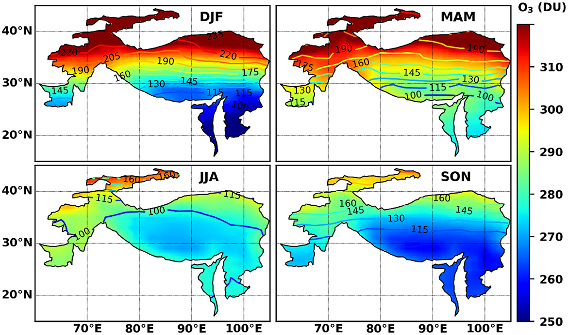
Figure 2. Seasonal mean TCO (DU) distribution in TP. The seasons are defined as spring: March–April–May (MAM), summer: June–July–August (JJA), autumn: September–October–November (SON), and winter: December–January–February (DJF). The overlaid contours show the climatology of tropopause pressure.

The high ozone concentration in the north TP during winter and spring is generally associated with vertical transport of ozone rich air by BDC (Weber et al., 2011). The upward transport of air by BDC can move ozone poor air into the lower stratosphere and downward transport of air can drive ozone rich air from stratosphere to upper troposphere (e.g., Ningombam et al., 2018). On the other hand, the surface temperature change and northward shift of subtropical westerly jet in the upper troposphere lift the local tropopause, and is a potential factor contributing to lower TCO, particularly at 75°-105° E in the south TP in winter (Bian, 2009; Liu et al., 2010; Zhang et al., 2014). Since the warming rate of the TP regions is higher in winter (Qin et al., 2009; Rangwala et al., 2009), lower TCO is found during the period.

There is a noticeable regional variation in seasonal distribution of TCO in TP. For example, the north TP shows higher TCO (≥310 DU) during winter and spring, and lower TCO (285–300 DU) during summer and autumn. The subtropical westerly jet plays a major role in blocking transport of ozone to north of the jet, which in turn increases the ozone concentration in the north TP. In the south, lower TCO ( ≤ 260 DU) is observed in winter and higher TCO (≥280 DU) in spring, which is mainly due to stratospheric-tropospheric dynamics (Liu et al., 2009). In the central TP, higher TCO (280–300 DU) is observed in winter and spring, and lower TCO (260–270 DU) in autumn. In addition, there is a significant difference in TCO values over the eastern and western TP in all seasons. For instance, the east TP shows 10–15 DU less TCO than that in the west, south of 35° N. The north TP shows higher TCO (310 DU) during winter and spring, and lower TCO (285–290 DU) in summer and autumn, consistent with the relatively stronger BDC in winter and spring.

Also, the variation in geopotential height is linked to the seasonal variation in temperature, which has a localized effect in the vertical movement of air mass over TP. Therefore, it influences the strength of tropospheric teleconnection patterns or climate modes and their impact on TCO distribution in TP. In general, during El Nino events, ENSO (index) and geopotential heights are negatively correlated over TP in winter; suggesting that the rise in tropopause height would lead to a reduction in TCO over TP (Li et al., 2020). However, there is no strong correlation between geopotential height and ENSO (index) and thus, no significant decrease in TCO is observed in other seasons.

Our results are consistent with those of previous analyses for the TBP and Tibet regions. For instance, Zou (1996) found the seasonal variation of 273–315 DU over the region 25.5°-40.5° N and 75°-105° E for the period 1979–1991. Likewise, Zhang et al. (2014) show 270–310 DU in winter and 270–290 DU in summer over the TBP region of 27.5°-37.5° N and 75°-105° E for the period 1980–2008. In a recent study, Zou et al. (2020) find a seasonal variation of 260–290 DU over Tibet within the region 27.5°-37.5° N and 75°-105° E during the period 2004–2019.

3.2. Interannual variability of TCO

The spatial distribution of yearly-averaged TCO in TP during the period 2005–2020 is shown in Supplementary Figure S2. The interannual variability of TCO is mostly governed by the yearly changes in local meteorology, solar activity, teleconnection patterns and other climate modes. For instance, large interannual variability is observed in 2005–2006, 2008–2009, 2014–2016 and 2018–2019 within the region 10°-38° N and 75°-105° E, which coincide with the solar cycles (i.e., the periodic rise and fall in solar activities over a time period of 11 years). The solar radiation makes changes in upper atmosphere, and then changes ozone concentration by photochemical reactions. In addition, absorption of solar radiation by O₃ in the stratosphere leads to change in the atmospheric thermal dynamics, and thus, the atmospheric circulation changes the ozone distribution there (Zhou et al., 2006). Again, these interannual changes also coincide with the ENSO events as evidenced by the enhanced TCO during the El Niño events in 2009–2010 (moderate), 2014–2015 (very strong) and 2018–2019 (weak), and reduced TCO during the La Niña events in 2008–2009 (weak), 2010–2011 (strong) and 2014–2015 (weak). The composite analysis of TCO during the El Niño, La Niña and normal years show that TCO in El Niño years is about 5–10 DU higher in the north TP with respect to normal years. Conversely, the change is very small during La Niña years and are about −2 DU (Supplementary Figure S3). Similar results on the effect of ENSO on TCO distribution in TBP can also be found in Han et al. (2001).

3.3. Spatial and temporal trends in TCO

Figure 3 shows the annual and seasonal trends in TCO estimated for the period 2005–2020. The estimated annual trends vary from 0.05 to −0.5 DU/yr. The annual trends show mostly negative values throughout the TP regions. The highest negative trends of about −0.5 DU/yr are found over Qaidam basin in the northeast, Hindu Kush Mountain in the west, and Tianshan Mountain in the north. Smallest negative trends are found in the southeast TP around Chittagong hill in Bangladesh and Garo hill in North-East India. There are large differences in the trends estimated for different seasons, and they vary from −0.6 to 0.2 DU/yr. For instance, positive trends are estimated (0.2 DU/yr) for most regions in TP during winter, although trends are slightly negative (about −0.2 DU/yr) in the east and west TP boundary regions. In spring, the trends are slightly positive in the southeast, whereas other regions show negative trends with the highest value of −0.5 DU/yr in Qaidam basin in the northeast TP. In summer and autumn, the trends are mostly negative, ranging from −0.2 DU/yr to −0.6 DU/yr, and the trends are relatively strong in autumn. These trends, however, are not statistically significant at the 95% confidence Interval in any season (e.g., Supplementary Figure S4 shows the statistical significance values for the estimated trends).

FIGURE 3

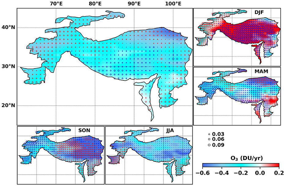
Figure 3. Annual and seasonal trends in TCO over TP for the period 2005–2020. The seasons are defined as spring: March–April–May (MAM), summer: June–July–August (JJA), autumn: September–October–November (SON), and winter: December–January–February (DJF). The overlaid open circles show the surface temperature (1,000 hPa, from ERA5) trends. Red and blue circles denote positive and negative trends in temperature, respectively. The size of the circle represents the magnitude of the trends.

We have also estimated the annual and seasonal mean (Supplementary Figure S4) and trend (Figure 4) in TCO over 20 urban sites in and around TP. The annual mean distribution of TCO is largest (330 ± 3.1 DU) over Uramqi and smallest (265 ± 2.1 DU) over Naypyitaw. The smallest negative annual trend (−0.01 ± 0.2 DU/yr) is found over Chittagong, but the highest (−0.42 ± 0.3 DU/yr) over Xinning, as listed in Supplementary Table S1. In general, the annual trends are negative over the entire TP though some seasonal trends are positive over some cities. For example, winter trends are positive over most cities, except Dushanbe, Tashkent, Bishkek, Almaty and Uramqi, where they show the highest negative trend in summer and smallest in winter, and the highest seasonal mean in winter and smallest in autumn. Small positive trends are found over Naypyitaw, Chittagong, Agartala, Silchar, Shillong, Thimphu, and Kathmandu in spring and winter, and these cities are near Bay of Bengal. Strong winds, high precipitation, high humidity and moderate air temperatures in this region make smaller annual mean TCO.

FIGURE 4

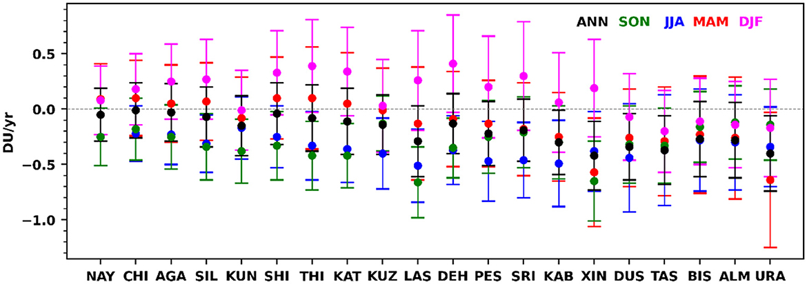
Figure 4. Annual and seasonal trends in TCO at different cities in TP for the period 2005–2020. The cities are arranged in ascending order in latitude and the details about city names and other are given in Supplementary Table S1. The seasons are defined as spring: March–April–May (MAM), summer: June–July–August (JJA), autumn: September–October–November (SON), and winter: December–January–February (DJF). The annually averaged data are represented by the black line (ANN).

In a similar study, Zhou et al. (2013) found a high negative trend with the highest value of −0.40 ± 0.10 DU/yr in January based on the TOMS/SBUV ozone data for the period 1979–2010 in TBP. In another study, Li et al. (2020) observed a negative trend of −0.56±0.21 DU/yr and −0.30 ± 0.11 DU/yr in winter and summer, respectively, for the period 1979–1996 in TBP. In a subsequent study, Zou et al. (2020) showed a negative trend in 1979–1996 and an increasing trend in 1997–2018 at 30° N−35° N, and an increasing trend of 0.37 DU/yr in the region 27.5° N−37.5° N, 75.50° E−105.5° E for the period 2005–2019. Our trend estimates are slightly different from the previous studies because the differences in region, data and period of analyses. For instance, Zou et al. (2020) found a positive trend of 0.021 ± 0.124 DU/yr in the annual averaged TCO in 2005–2019 based on the OMI data over TBP (27.5°-37.5° N and 75.5°-105.5° E). Also, our estimates of the highest and lowest reduction in TCO during winter/spring and autumn, respectively, are also consistent with the results of Zou (1996) and Zhang et al. (2014) for the TBP regions. Studies show that the thermodynamical processes associated with the warming of TP are responsible for about 50% reduction in TCO during winter in TBP (Zhang et al., 2014). In addition, the solar minimum has also affected TCO to be relatively lower in the past decade. We have also analyzed the surface temperature trends and found that the TCO trends are negatively associated with that of temperature (the overlaid circles in Figure 3). This is particularly evident in the seasonal trends in TCO and temperature in winter and spring. We observe a TP-wide cooling and warming in autumn and winter, respectively, up to 0.09°C/yr.

3.4. Multiple linear regression of TCO

We have used a MLR to find the trends in TCO and contribution of different factors to TCO change in TP. To perform the regression, we have tested the multi-collinearity of predictors used and found that they do not have significant multi-collinearity. Additionally, we also performed the analysis of Variance Inflation Factor to make sure that the multi-collinearity among the predictors is not significant. We have used the normalized anomaly of yearly averaged TCO with mean and standard deviation of 0 and 1, respectively, which are widely used in the trend studies, as the variability in TCO has a strong seasonal dependence (Staehelin et al., 2001; Poulain et al., 2016; WMO (World Meteorological Organization), 2018). Figure 5 shows the temporal evolution of TCO and the MLR fit for the period 2005–2020. The yearly (monthly) averaged TCO shows an R² value of 0.72 (0.5). Azen and Budescu (2003) proposed the dominance analysis to find the relative importance of predictors based on the additional contribution of a predictor in all subsets with the individual contribution. We have used the dominance analysis to determine the importance of each predictor used in the regression. The regression coefficient indicates the positive or negative contribution of each predictor to the TCO changes.

FIGURE 5

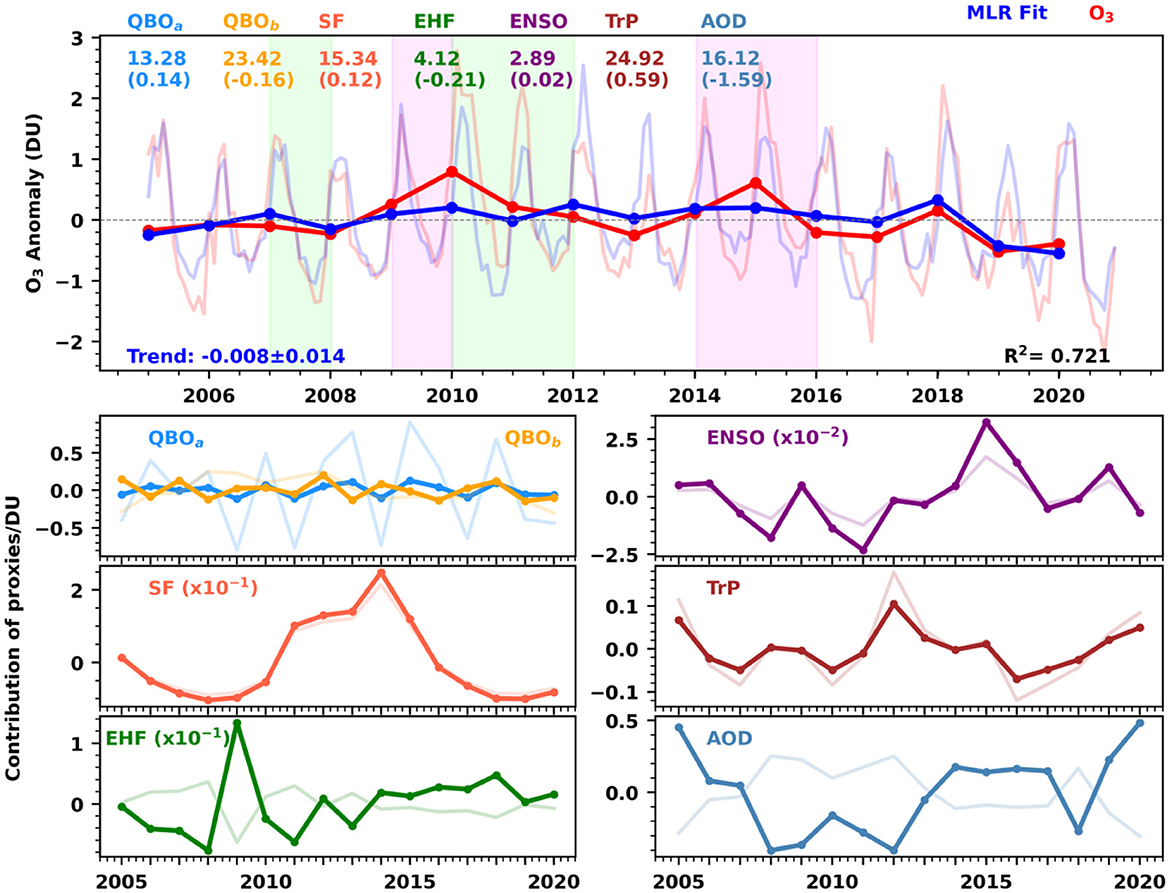
Figure 5. (Top panel) Regression result based on the normalized TCO over TP for the period 2005–2020. Red line is the annually averaged anomaly of TCO and blue line represents the MLR fit. The numerical values indicate the relative importance of each contributor estimated using the Dominance Analysis. The values in brackets indicate the regression coefficient of each predictor. The light-colored red and blue lines indicate the monthly averaged time series of TCO and MLR fit, respectively. The lime-color shade represents strong La-Niña and light-magenta shade represents strong El Niño events during the period of study. (Bottom panels) The thick lines represent the contribution of each predictor for the period 2005–2020. The thin lines in the background represent the normalized distribution of predictors used. Here, QBO_a and QBO_b are the indices of Quasi-Biennial Oscillation indices 10 and 30 hPa, respectively, EHF is the Eddy Heat Flux at 100 hPa, SF is the Solar Flux, ENSO is the El-Niño Southern Oscillation Index, TrP is the tropopause Pressure and AOD is the Aerosol Optical Depth.

The trend in TCO is about −0.015 ± 0.16 DU/yr as estimated from the yearly averaged data, which is close to that estimated from the linear regression (−0.0087 ± 0.09 DU/yr). The analyses show that the tropopause height has the strongest effect (25.44%); suggesting that the lower tropopause makes higher TCO. The QBO_b has the second highest contribution to the ozone change (23.42%), followed by aerosols (AOD, 16.12%) and solar flux (15.34%). The TCO change during the solar maximum and minimum are clearly shown in figure, e.g., TCO is lower during the solar minimum period. The heat flux explains the effect of BDC from the tropics to mid-latitudes, and there is a statistically significant linear relationship between TCO and EHF at 100 hPa for the tropical and polar regions (Weber et al., 2011). Conversely, the aerosols mostly have a negative relationship with the TCO changes. The value of TCO is lowest (−2DU) in the autumn 2020, which can be due to the combined effect of lowest solar flux and the highest tropopause in that year. Note that stratospheric ozone plays a key role in the height of tropopause by radiative heating, and ozone diagnostics are also subjected to local meteorology and the stratospheric circulation (Seidel and Randel, 2006; Austin and Reichler, 2008).

4. Conclusions

We have examined the spatial and temporal changes in TCO over Third Pole and 20 cites in and around the region. Observed TCO varies with latitude, longitude, altitude and meteorological conditions. Large variation in TCO is found in higher latitudes with the highest ozone there, and significant longitudinal variability is observed at lower latitudes. Relatively high temporal variability is found at the lower latitudes in seasonal to interannual scales than those at the higher latitudes; showcasing the influence of atmospheric circulation in TCO distribution. Most of the TCO variability in the region is driven by the changes in tropopause height and atmospheric dynamics. In general, the seasonal trends are negative in most cities and over TP, except in winter. The highest negative trend of −0.42 ± 0.3 DU/yr and the lowest of −0.01 ± 0.2 DU/yr are found for Xining and Chittagong, respectively, with respect to the yearly averaged data. The negative trends in TCO over the nearby populated regions (cities) suggest the possibility of enhanced solar incidence and changes in surface temperature. Change in the temperature in the high latitude glacier TP region is a concern for the water security of south Asia. Therefore, it is inevitable to continuously monitor and analyze TCO in the region, as performed here, for the assessment of public health and climate change in the region.

Data availability statement

The original contributions presented in the study are included in the article/Supplementary material, further inquiries can be directed to the corresponding author. Publicly available data can be downloaded from: Ozone: www.temis.nl Solar Cycle: https://www.ngdc.noaa.gov/stp/solar/flux.html QBO: https://www.geo.fu-erlin.de/en/met/ag/strat/produkte/qbo/ ENSO: https://psl.noaa.gov/enso/mei AOD: https://gmao.gsfc.nasa.gov/reanalysis/MERRA-2/ Tropopause pressure: https://www.ncep.noaa.gov/ Eddy heat flux and temperature data: https://www.ecmwf.int/en/forecasts/datasets/reanalysis-datasets/era5 Topography: https://visibleearth.nasa.gov/collection/1484/blue-marble.

Author contributions

JK: conceptualization, methodology, software, validation, formal analysis, investigation, resources, data curation, writing—original draft, writing—review and editing, visualization, supervision, project administration, and funding acquisition. BS and GG: methodology, software, validation, formal analysis, investigation, data curation, visualization, and writing—original draft. All authors contributed to the article and approved the submitted version.

Acknowledgments

We thank the Director, Indian Institute of Technology Kharagpur (IIT Kgp), Chairman of CORAL IIT Kgp and the Ministry of Education (MoE) for facilitating the study. The authors also thank the TOMS/OMI/GOME-2B data providers. BS acknowledges his IIT Kgp Doctoral Scholarship for Foreign Students. GG acknowledges Department of Science and Technology, Ministry of Science and Technology, India for the INSPIRE fellowship for his Doctoral study at IIT KGP.

Conflict of interest

The authors declare that the research was conducted in the absence of any commercial or financial relationships that could be construed as a potential conflict of interest.

Publisher's note

All claims expressed in this article are solely those of the authors and do not necessarily represent those of their affiliated organizations, or those of the publisher, the editors and the reviewers. Any product that may be evaluated in this article, or claim that may be made by its manufacturer, is not guaranteed or endorsed by the publisher.

Supplementary material

The Supplementary Material for this article can be found online at: https://www.frontiersin.org/articles/10.3389/fclim.2023.1129660/full#supplementary-material

References

Austin, J., and Reichler, T. J. (2008). Long-term evolution of the cold point tropical tropopause: simulation results and attribution analysis. J. Geophys. Res. Atmos. 113:D00B10. doi: 10.1029/2007JD009768

CrossRef Full Text | Google Scholar

Azen, R., and Budescu, D. V. (2003). The dominance analysis approach for comparing predictors in multiple regression. Psychol. Methods 8, 129. doi: 10.1037/1082-989X.8.2.129

PubMed Abstract | CrossRef Full Text | Google Scholar

Bai, K., Chang, N. B., Yu, H., and Gao, W. (2016). Statistical bias correction for creating coherent total ozone record from OMI and OMPS observations. Remote Sens. Environ. 182, 150–168. doi: 10.1016/j.rse.2016.05.007

CrossRef Full Text | Google Scholar

Bian, J. (2009). Features of ozone mini-hole events over the Tibetan Plateau. Adv. Atmos. Sci. 26, 305–311. doi: 10.1007/s00376-009-0305-8

CrossRef Full Text | Google Scholar

Bonasoni, P., Cristofanelli, P., Marinoni, A., Vuillermoz, E., and Adhikary, B. (2012). Atmospheric pollution in the Hindu Kush–Himalaya region. Mt. Res. Dev. 32, 468–479. doi: 10.1659/MRD-JOURNAL-D-12-00066.1

PubMed Abstract | CrossRef Full Text | Google Scholar

Callies, J., Corpaccioli, E., Eisinger, M., Lefebvre, A., Munro, R., Perez-Albinana, A., et al. (2003). GOME-2: The ozone instrument onboard the European METOP satellites. Polariz. Sci. Rem. Sens. 5158, 1–11. doi: 10.1117/12.504475

CrossRef Full Text | Google Scholar

Chipperfield, M. P., Dhomse, S. S., Feng, W., McKenzie, R. L., Velders, G. J., and Pyle, J. A. (2015). Quantifying the ozone and ultraviolet benefits already achieved by the Montreal Protocol. Nat. Commun. 6, 1–8. doi: 10.1038/ncomms8233

PubMed Abstract | CrossRef Full Text | Google Scholar

Cong, Z., Kawamura, K., Kang, S., and Fu, P. (2015). Penetration of biomass-burning emissions from South Asia through the Himalayas: new insights from atmospheric organic acids. Sci. Rep. 5, 1–7. doi: 10.1038/srep09580

PubMed Abstract | CrossRef Full Text | Google Scholar

de Laat, A. T. J., van Weele, M., and van der, A. R. J. (2017). Onset of stratospheric ozone recovery in the Antarctic ozone hole in assimilated daily total ozone columns. J. Geophys. Res. 122, 11880–11899. doi: 10.1002/2016JD025723

CrossRef Full Text | Google Scholar

Eskes, H. J., Velthoven, P. V., Valks, P. J. M., and Kelder, H. M. (2003). Assimilation of GOME total-ozone satellite observations in a three-dimensional tracer-transport model. Q. J. R. Meteorol. Soc. 129, 1663–1681. doi: 10.1256/qj.02.14

CrossRef Full Text | Google Scholar

Forster, P. M., and Shine, K. P. (1997). Radiative forcing and temperature trends from stratospheric ozone changes. J. Geophys. Res. Atmos. 102, 10841–10855. doi: 10.1029/96JD03510

CrossRef Full Text | Google Scholar

Gautam, A. P., Webb, E. L., Shivakoti, G. P., and Zoebisch, M. A. (2003). Land use dynamics and landscape change pattern in a mountain watershed in Nepal. Agric. Ecosyst. Environ. 99, 83–96. doi: 10.1016/S0167-8809(03)00148-8

CrossRef Full Text | Google Scholar

Han, Z., Chongping, J., Libo, Z, Wei, W., and Yongxiao, J. (2001). ENSO signal in total ozone over Tibet. Adv. Atmos. Sci. 18, 231–238. doi: 10.1007/s00376-001-0016-2

CrossRef Full Text | Google Scholar

IPCC (2013). Climate Change 2013: The Physical Science Basis. Contribution of Working Group I to the Fifth Assessment Report of the Intergovernmental Panel on Climate Change, eds T. F. Stocker, D. Qin, G. K. Plattner, M. Tignor, S. K. Allen, J. Boschung, et al. (Cambridge, United Kingdom; New York, NY: Cambridge University Press), 1535.

Google Scholar

Kang, S., Zhang, Q., Qian, Y., Ji, Z., Li, C., Cong, Z., et al. (2019). Linking atmospheric pollution to cryospheric change in the Third Pole region: current progress and future prospects. Natl. Sci. Rev. 6, 796–809. doi: 10.1093/nsr/nwz031

PubMed Abstract | CrossRef Full Text | Google Scholar

Kroon, M., Petropavlovskikh, I., Shetter, R., Hall, S., Ullmann, K., Veefkind, J. P., et al. (2008). OMI total ozone column validation with Aura-AVE CAFS observations. J. Geophys. Res. Atmos. 113:D16S28. doi: 10.1029/2007JD008795

CrossRef Full Text | Google Scholar

Kuttippurath, J., Kumar, P., Nair, P. J., and Pandey, P. C. (2018). Emergence of ozone recovery evidenced by reduction in the occurrence of Antarctic ozone loss saturation. npj Clim. Atmos. Sci. 1, 1–8. doi: 10.1038/s41612-018-0052-6

CrossRef Full Text | Google Scholar

Kuttippurath, J., Lefèvre, F., Pommereau, J. P., Roscoe, H. K., Goutail, F., Pazmino, A., et al. (2013). Antarctic ozone loss in 1979–2010: first sign of ozone recovery. Atmos. Chem. Phys. 13, 1625–1635. doi: 10.5194/acp-13-1625-2013

CrossRef Full Text | Google Scholar

Kuttippurath, J., and Nair, P. J. (2017). The signs of Antarctic ozone hole recovery. Sci. Rep. 7, 1–8. doi: 10.1038/s41598-017-00722-7

PubMed Abstract | CrossRef Full Text | Google Scholar

Levelt, P. F., van den Oord, G. H., Dobber, M. R., Malkki, A., Visser, H., De Vries, J., et al. (2006). The ozone monitoring instrument. IEEE Trans. Geosci. Remote Sens. 44, 1093–1101. doi: 10.1109/TGRS.2006.872333

CrossRef Full Text | Google Scholar

Li, Y., Chipperfield, M. P., Feng, W., Dhomse, S. S., Pope, R. J., Li, F., et al. (2020). Analysis and attribution of total column ozone changes over the Tibetan Plateau during 1979–2017. Atmos. Chem. Phys. 20, 8627–8639. doi: 10.5194/acp-20-8627-2020

CrossRef Full Text | Google Scholar

Lin, J. T. (2012). Satellite constraint for emissions of nitrogen oxides from anthropogenic, lightning and soil sources over East China on a high-resolution grid. Atmos. Chem. Phys. 12, 2881–2898. doi: 10.5194/acp-12-2881-2012

CrossRef Full Text | Google Scholar

Liu, C., Liu, Y., Cai, Z., Gao, S., Bian, J., Liu, X., et al. (2010). Dynamic formation of extreme ozone minimum events over the Tibetan Plateau during northern winters 1987–2001. J. Geophys. Res. Atmos. 115:D18311. doi: 10.1029/2009JD013130

CrossRef Full Text | Google Scholar

Liu, C., Liu, Y., Cai, Z., Gao, S., Lu, D., and Kyrola, E. (2009). A Madden Julian Oscillation triggered record ozoneminimum over the Tibetan. Geophys. Res. Lett. 36, L15830. doi: 10.1029/2009GL039025

CrossRef Full Text | Google Scholar

Loyola, D. G., Koukouli, M. E., Valks, P., Balis, D. S., Hao, N., Van Roozendael, M., et al. (2011). The GOME-2 total column ozone product: retrieval algorithm and ground-based validation. J. Geophys. Res. Atmos. 116, 1–11. doi: 10.1029/2010JD014675

CrossRef Full Text | Google Scholar

Nair, P. J., Froidevaux, L., Kuttippurath, J., Zawodny, J. M., Russell III, J. M., Steinbrecht, W., et al. (2015). Subtropical and midlatitude ozone trends in the stratosphere: implications for recovery. J. Geophys. Res. Atmos. 120, 7247–7257. doi: 10.1002/2014JD022371

CrossRef Full Text | Google Scholar

Ningombam, S. S., Vemareddy, P., and Song, H. J. (2018). The recent signs of total column ozone recovery over mid-latitudes: the effects of the Montreal Protocol mandate. J Atmos. Sol. Terr. Phys. 178, 32–46. doi: 10.1016/j.jastp.2018.05.011

CrossRef Full Text | Google Scholar

Pazmiño, A., Godin-Beekmann, S., Hauchecorne, A., Claud, C., Khaykin, S., Goutail, F., et al. (2018). Multiple symptoms of total ozone recovery inside the Antarctic vortex during austral spring, Atmos. Chem. Phys. 18, 7557–7572. doi: 10.5194/acp-18-7557-2018

CrossRef Full Text | Google Scholar

Poulain, V., Bekki, S., Marchand, M., Chipperfield, M., Khodri, M., Lef?vre, F., et al. (2016). Evaluation of the inter-annual variability of stratospheric chemical composition in chemistry-climate models using ground-based multi species time. J. Atmos. Sol. Terr. Phys. 145, 61–84. doi: 10.1016/j.jastp.2016.03.010

CrossRef Full Text | Google Scholar

Qin, J., Yang, K., Liang, S., and Guo, X. (2009). The altitudinal dependence of recent rapid warming over the Tibetan Plateau. Clim. Change 97, 321–327. doi: 10.1007/s10584-009-9733-9

CrossRef Full Text | Google Scholar

Qiu, J. (2008). China: the third pole. Nature 454, 393–396. doi: 10.1038/454393a

PubMed Abstract | CrossRef Full Text | Google Scholar

Randel, W. J., and Park, M. (2006). Deep convective influence on the Asian summer monsoon anticyclone and associated tracer variability observed with Atmospheric Infrared Sounder (AIRS). J. Geophys. Res. Atmos. 111:D12314. doi: 10.1029/2005JD006490

CrossRef Full Text | Google Scholar

Rangwala, I., Miller, J. R., and Xu, M. (2009). Warming in the Tibetan Plateau: possible influences of the changes in surface water vapor. Geophys. Res. Lett. 36:LO6703. doi: 10.1029/2009GL037245

CrossRef Full Text | Google Scholar

Schoeberl, M. R., Douglass, A. R., Hilsenrath, E., Bhartia, P. K., Beer, R., Waters, J. W., et al. (2006). Overview of the EOS Aura mission. IEEE Trans. Geosci. Remote Sens. 44, 1066–1074. doi: 10.1109/TGRS.2005.861950

CrossRef Full Text | Google Scholar

Seidel, D. J., and Randel, W. J. (2006). Variability and trends in the global tropopause estimated from radiosonde data. J. Geophys. Res. Atmos. 111, 1–17. doi: 10.1029/2006JD007363

CrossRef Full Text | Google Scholar

Solomon, S., Ivy, D. J., Kinnison, D., Mills, M. J., Neely, R. R., and Schmidt, A. (2016). Emergence of healing in the Antarctic ozone layer. Science 353, 269–274. doi: 10.1126/science.aae0061

PubMed Abstract | CrossRef Full Text | Google Scholar

Staehelin, J., Harris, N. R. P., Appenzeller, C., and Eberhard, J. (2001). Ozone trends: A review. Rev. Geophys. 39, 231–290. doi: 10.1029/1999RG000059

CrossRef Full Text | Google Scholar

Tian, W., Chipperfield, M. P., and Huang, Q. (2008). Effects of the Tibetan Plateau on total column ozone distribution. Tellus B Chem. Phys. Meteorol. 60, 622–635. doi: 10.1111/j.1600-0889.2008.00338.x

CrossRef Full Text | Google Scholar

Veefkind, J. P., de Haan, J. F., Brinksma, E. J., Kroon, M., and Levelt, P. F. (2006). Total ozone from the Ozone Monitoring Instrument (OMI) using the DOAS technique. IEEE Trans. Geosci. Remote. Sens. 44, 1239–1244. doi: 10.1109/TGRS.2006.871204

PubMed Abstract | CrossRef Full Text | Google Scholar

Weber, M., Coldewey-Egbers, M., Fioletov, V. E., Frith, S. M., Wild, J. D., Burrows, J. P., et al. (2018). Total ozone trends from 1979 to 2016 derived from five merged observational datasets–the emergence into ozone recovery. Atmos. Chem. Phys. 18, 2097–2117. doi: 10.5194/acp-18-2097-2018

CrossRef Full Text | Google Scholar

Weber, M., Dikty, S., Burrows, J. P., Garny, H., Dameris, M., Kubin, A., et al. (2011). The Brewer-Dobson circulation and total ozone from seasonal to decadal time scales. Atmos. Chem. Phys. 11, 11221–11235. doi: 10.5194/acp-11-11221-2011

CrossRef Full Text | Google Scholar

Wester, P., Mishra, A., and Mukherji, A. Shrestha, A. B. (eds), (2019). The Hindu Kush Himalaya Assessment: Mountains, Climate Change, Sustainability and People. Cham: Nature Switzerland AG. doi: 10.1007/978-3-319-92288-1

CrossRef Full Text | Google Scholar

WMO (World Meteorological Organization). (2018). Scientific Assessment of Ozone Depletion: 2018, Global Ozone Research and Monitoring Project - Report No. 58. Geneva: World Meteorological Organization. p. 588.

Google Scholar

Xu, W., Lin, W., Xu, X., Tang, J., Huang, J., Wu, H., et al. (2016). Long-term trends of surface ozone and its influencing factors at the Mt Waliguan GAW station, China–Part 1: overall trends and characteristics. Atmos. Chem. Phys. 16, 6191–6205. doi: 10.5194/acp-16-6191-2016

CrossRef Full Text | Google Scholar

Yao, T., Thompson, L. G., Mosbrugger, V., Zhang, F., Ma, Y., Luo, T., et al. (2012). Third pole environment (TPE). Environ. Dev. 3, 52–64. doi: 10.1016/j.envdev.2012.04.002

CrossRef Full Text | Google Scholar

Zeng, G., Pyle, J. A., and Young, P. J. (2008). Impact of climate change on tropospheric ozone and its global budgets. Atmos. Chem. Phys. 8, 369–387. doi: 10.5194/acp-8-369-2008

CrossRef Full Text | Google Scholar

Zhang, J., Tian, W., Xie, F., Tian, H., Luo, J., Zhang, J., et al. (2014). Climate warming and decreasing total column ozone over the Tibetan Plateau during winter and spring. Tellus B Chem. Phys. Meteorol. 66, 23415. doi: 10.3402/tellusb.v66.23415

CrossRef Full Text | Google Scholar

Zhou, L., Zou, H., Ma, S., and Li, P. (2013). The Tibetan ozone low and its long-term variation during 1979–2010. Acta Meteorol. Sin. 27, 75–86. doi: 10.1007/s13351-013-0108-9

CrossRef Full Text | Google Scholar

Zhou, S., and Zhang, R. (2005). Decadal variations of temperature and geopotential height over the Tibetan Plateau and their relations with Tibet ozone depletion. Geophys. Res. Lett. 32, 109–127. doi: 10.1029/2005GL023496

CrossRef Full Text | Google Scholar

Zhou, X., Li, W., Chen, L., and Liu, Y. (2006). Study on ozone change over the Tibetan Plateau. Acta Meteorologica Sinica 20, 129–143.

Google Scholar

Zou, H. (1996). Seasonal variation and trends of TOMS ozone over Tibet. Geophys. Res. Lett. 23, 1029–1032. doi: 10.1029/96GL00767

CrossRef Full Text | Google Scholar

Zou, M., Xiong, X., Wu, Z., and Yu, C. (2020). Ozone trends during 1979–2019 over Tibetan Plateau derived from satellite observations. Front. Earth Sci. 8, 579624. doi: 10.3389/feart.2020.579624

CrossRef Full Text | Google Scholar