TRANSLATE: standardized climate projections for Ireland

1. Introduction

Within government and private-sector institutions, and among the general public, there is growing awareness of the risks of future climate change—partly due to climate model predictions, and partly to increasingly robust observational evidence of recent and current climate change [The Royal Society (UK), National Academy of Sciences (USA), 2020]. In Ireland, the development of climate resilience is channeled through the National Adaptation Frameworks (NAFs) (Department of Communications, Climate Action and Environment, Government of Ireland, 2018). The NAF focusses on ensuring that adaptation measures are taken at all levels of government to prepare Ireland for the impacts of climate change. As mandated by the NAF, each of the 31 Local Authority administrations in Ireland has their own Climate Change Adaptation Strategy.¹ These documents report that the main hazards of concern are heavy rainfall and associated flooding, heatwaves, drought, and storm events, all of which can affect the provision of local government and other utility services. Local Authorities and utility service providers need to understand how climate change will affect their activities, and so there is increasing demand for reliable climate projections in order to plan and implement suitable adaptation and mitigation measures.

Given this context, the TRANSLATE project² was established by the Irish national meteorological service, Met Éireann, in 2021 to produce standardized climate projections for Ireland, as a basis for the provision of other more wide-ranging climate services, and to support activities such as hydrological modeling. This paper describes the main principles and methods used to produce the first set of such projections and shows a small but indicative sample of the results obtained. Our work was guided to some extent by similar projects undertaken by other geographically small countries, such as UKCP18 in the UK (Lowe et al., 2018; Murphy et al., 2018), KNMI'14 in the Netherlands (Van den Hurk et al., 2014; Lenderink et al., 2015), and CH2018 in Switzerland (CH2018, 2018).

Many other countries or regions have also developed their own national climate scenarios based on CMIP global simulations, and some of these are listed in Supplementary Table S1. Ruosteenoja et al. (2016) describe downscaling CMIP5 GCM projections for Finland as an experimental extension of the more operationally oriented ACCLIM project, which derived climate projections for Finland from earlier CMIP3 simulations. These projections were updated by Ruosteenoja and Jylhä (2021) to use the latest CMIP6 shared socioeconomic pathway (SSP) scenarios, but without any downscaling. In Austria, the ÖKS15 project (Chimani et al., 2016) used 13 EURO-CORDEX regional models to downscale global simulations from two CMIP5 scenarios to the end of the 21st century. Technical aspects of the Norwegian climate projections are described by Hanssen-Bauer et al. (2017), while the utility and value of such projections is demonstrated by how they are disseminated and used to develop a “chain” of climate services, as reported by Nilsen et al. (2022). Similar projects undertaken by other nations are not cited in the interest of space, while no doubt there are others that we are unaware of, especially those that remain at the level of research projects, or where the information generated is available only in the local languages or simply not converted into publicly accessible products. Given the variety of approaches even among those few countries mentioned above, however, it is clear that the generation of standardized national climate projections does not have a “one size fits all” solution.

Most localized climate projections depend on a chain of future climate simulations that starts with ensembles of relatively coarse-resolution global climate models (GCMs). These may be dynamically downscaled to smaller, regional domains by ensembles of higher-resolution regional climate models (RCMs) each nested within one or more of the GCMs. High-resolution RCMs can also be nested within coarser ones, as done by Nolan (2015) and Nolan et al. (2017) for domains centered on Ireland (see, e.g., Figure 1.2 and related text in Nolan, 2015). Further statistical post-processing (e.g., detrending, bias-correction, and further downscaling), leads to a distilled reference set of climate data and spatial maps representing annual, seasonal, monthly, or even daily statistics for a range of variables at different time-periods or thresholds in the future, under different external forcing scenarios. The reference set typically encompasses alternative climates from both the lower and higher climate sensitivity ranges, as determined by the spread of the underlying ensembles.

The resulting set of climate scenarios described in this document could be viewed as spanning a small 3-dimensional matrix, as shown in Figure 1, which is adapted from Figure 10.9 of the latest Swiss climate scenario report (CH2018, 2018). In this view, future time-periods (specifically 2021–2050, 2041–2070, and 2071–2100) lie along one dimension. A few external forcing scenarios form a second dimension. For the first TRANSLATE implementation, these are Representative Concentration Pathways (RCPs) 2.6, 4.5 and 8.5, as used for the Coupled Model Intercomparison project Phase 5 (CMIP5; Taylor et al., 2012). These three scenarios can be viewed as a measure of future forcing uncertainty. The third dimension in Figure 1 spans a set of three different “climate sensitivity” levels among the ensemble of RCMs, where climate sensitivity is measured by the mean surface temperature change over Ireland during 2071–2100 under RCP4.5 and RCP8.5, as simulated by each ensemble member. These low, medium and high-sensitivity sub-ensembles provide a measure, however crude, of model response uncertainty. All changes are measured relative to the reference period 1976–2005, which was chosen to correspond with the last 30 years of the CMIP5 “historical” period.

FIGURE 1

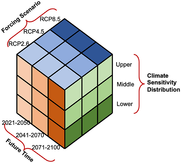
Figure 1. Schematic of how future climate uncertainties can be accommodated in a limited set of possible climates, adapted from Figure 10.9 of CH2018 (CH2018 Report, 2018). Each sub-cube shown corresponds to an ensemble of long-term climate simulations. Different RCP emission scenarios represent forcing uncertainty, while the climate sensitivity axis represents response uncertainty.

The different climates corresponding to each of the 27 sub-cubes in Figure 1 were supplemented by a further time-slicing approach, which aggregated the forcing scenarios and future time periods into three new “warming level” scenarios, centered on the years when each underlying GCM crossed global surface temperature change thresholds of 1.5, 2.0 and 2.5°C, resp. A template for constructing such threshold-based climate scenarios is provided by Vautard et al. (2014), and Supplementary Figure S1 shows a sample case of how it was done for TRANSLATE. In practice, in almost all RCP scenarios, global temperature crosses at least the 1.5°C threshold, while the 2.5°C threshold is crossed in all the RCP8.5 simulations and most of the RCP4.5 ones.

The rest of this paper describes how the 27 different climates of Figure 1 (along with the 3 temperature threshold climates) were constructed by de-trending, bias-correcting, and further statistically downscaling the raw RCM output from two separate sets of simulations. Some sample results are provided for illustrative purposes.

2. Methods

2.1. Two different RCM ensembles

The first effort to produce standardized future climate projections for Ireland begins with the separate sets of downscaled ensemble-RCM simulations from Nolan and Flanagan (2020; henceforth N&F), and the EURO-CORDEX project.³ Both sets of simulations were embedded in CMIP5 GCMs (see Figure 2), with four GCMs used in common. However, both projects used completely different RCMs, different grid spacing, and had different numbers of ensemble members (see Table 1 for a summary of some key differences). Note that we used the EURO-CORDEX simulations with ~12 km grid spacing; those EURO-CORDEX runs with ~50 km grid spacing had too few points to capture adequate detail over Ireland. In contrast, the N&F simulations were at 4 km grid-spacing. Thus, both sets of simulations produced what could be viewed as independent versions of the 27 sub-climates depicted in Figure 1.

FIGURE 2

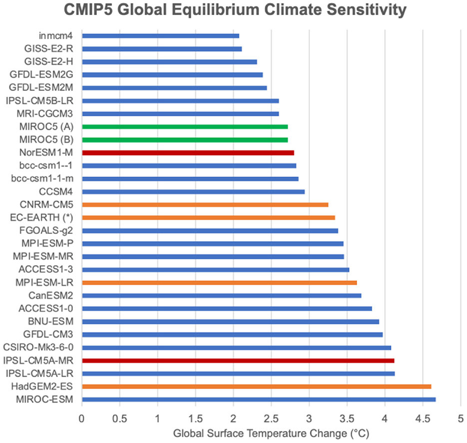
Figure 2. Ordered list of CMIP5 model ECS values, aggregated from Table 7.SM.5 of the IPCC AR6 report, Vol. 1: (https://www.ipcc.ch/report/ar6/wg1/downloads/report/IPCC_AR6_WGI_Chapter_07_Supplementary_Material.pdf). The green bars represent models used for RCM downscaling by Nolan and Flanagan (2020), the red bars represent models used for RCM downscaling by EURO-CORDEX, while the orange bars represent models used by both. The blue bars represent models not used by TRANSLATE because no high-resolution RCM-downscaling of them was available over Ireland. (^*) EC-EARTH model sensitivity was estimated separately.

TABLE 1

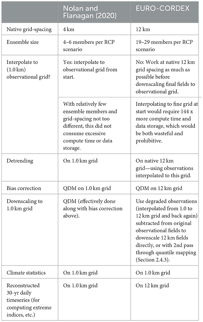
Table 1. Comparison of how the Nolan and Flanagan (2020) and EURO-CORDEX downscaled ensembles of RCMs are different, and handled differently by TRANSLATE.

Regarding the N&F RCMs, the choice of model physics and parameterization schemes was informed by short-term validation experiments and the recommendations of the respective RCM development team. For example, the N&F WRF simulations did not include a convection parameterization scheme (convection resolving) while the COSMO-CLM5 simulations utilized the Mass Flux Tiedtke parameterization scheme (Tiedtke, 1989). An overview of the N&F RCM configurations is provided by Nolan et al. (2017) and Nolan and Flanagan (2020). The N&F RCM configurations were validated by downscaling European Center for Medium-Range Weather Forecasts (ECMWF) ERA-Interim reanalyzes for multi-decadal time periods and comparing the output with observational data. For an in-depth validation of the RCMs, see Nolan et al. (2017), Flanagan et al. (2019), Werner et al. (2019), Flanagan and Nolan (2020), and Nolan and Flanagan (2020), whose results confirm that the output of the RCMs exhibit reasonable and realistic features, as documented in the historical data record, and consistently demonstrate improved skill over the GCMs and low-resolution RCMs in the simulation of multiple fields (e.g., precipitation and near-surface temperature, wind, humidity and radiation). Nolan et al. (2017) analyzed a larger ensemble of RCMs (both COSMO-CLM and WRF) with different grid spacings (18, 7, 6, 4, 2, and 1.5 km) and found that the RCMs demonstrated a general stepwise increase in skill with increased model resolution. Furthermore, it was shown that heavy precipitation events are more accurately resolved by the higher spatial resolution RCM data. However, it was found that although the RCM accuracy increased with higher spatial resolution, reducing the horizontal grid spacing below 4 km provided relatively little added value (Nolan et al., 2017). These results, and the requirement for a large RCM ensemble for analysis of climate projection uncertainty, informed the N&F RCM 4 km experiment setup.

2.2. Historical observations

High-resolution (~1.0 km grid-spacing) gridded observations of daily mean, minimum, and maximum surface air temperature (at 2 m height) for the Republic of Ireland, and daily precipitation over all Ireland were provided by Met Éireann spanning the reference historical period 1976–2005. The production of these datasets is described by Walsh (2016, 2017), while the time-period available has expanded from 1981–2010 to span 1961–2014. The temperature fields were supplemented by temperature observations at 5 km grid spacing over Northern Ireland (the northeastern part of the island and part of the UK) from the UK Met. Office's CEDA archive (Hollis et al., 2018). Standard bilinear interpolation was used to patch the temperature data across the border between the Republic of Ireland and Northern Ireland.

Those 30-year high-resolution gridded observations of daily minimum, maximum and mean air surface temperature and daily precipitation were used to validate the corresponding variables in RCM output for the same historical period (1976–2005), and to facilitate downscaling and bias-correction of all future projections, as described below. Ensembles of reconstructed (i.e., detrended and bias-corrected) 30-year daily timeseries of those four variables provide the basis for each of the 27 representative climates shown in Figure 1.

Note that while all model output included gridded values over both land and sea, the observational temperature data were provided over land only. The discontinuities across the coastline introduced some difficulties when using simple interpolation, since offshore grid-points with “missing data” could then contaminate neighboring onshore points by treating them as “missing” too. The interpolation algorithm was modified to work around this issue by interpolating from available land points only.

2.3. Climate sensitivity decomposition

For any given RCP forcing scenario and for any future time-period, the decomposition of the “climate sensitivity” axis in Figure 1 can be done in different ways. Prior to making a final choice, it is worth considering the “equilibrium climate sensitivity” (ECS) of the different CMIP5 global models, as shown in Figure 2. ECS is the equilibrium global-mean surface temperature change that occurs in response to instantaneous doubling of CO₂ concentrations. The green, red, and orange bars represent models that were used for high-resolution dynamical downscaling with RCMs over Ireland by N&F, EURO-CORDEX, or both, and so are incorporated into TRANSLATE. The models available for use by TRANSLATE are reasonably well-distributed among the different ECS values, although the models with lowest ECS (e.g., the GISS and GFDL models) are not available, since they were not downscaled over Ireland by any RCM with adequate grid spacing. This “low-sensitivity” gap should be remembered when analyzing the distribution of TRANSLATE results.

For the purposes of TRANSLATE, however, the climate sensitivity of each model over Ireland is more relevant than the global ECS. Figure 3 shows the mean surface temperature changes over Ireland from the RCM ensemble means from 3 different future scenarios and time-periods, all relative to 1976–2005. Figure 3A is for the N&F ensemble; Figure 3B is for the EURO-CORDEX ensemble. For all 3 metrics in both ensembles, the HadGEM2-ES model is clearly the most sensitive, while the MPI-ESM-LR model is the least sensitive—even though MPI-ESL-LR is among the more sensitive models as measured by the global ECS metric (Figure 2). The difference in the projected mean temperature changes over Ireland under RCP8.5 by the end of the century between the most (HadGEM2-ES) and the least (MPI-ESM-LR) sensitive models is almost 1.7°C (3.63° vs. 1.94°C).

FIGURE 3

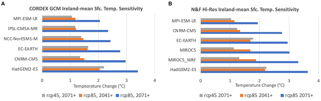
Figure 3. CMIP5 global models used by TRANSLATE, ranked by the mean surface temperature change over Ireland from the RCM ensemble-mean under the RCP8.5 scenario for the period 2071–2100 (blue bars). (A) is from the Nolan and Flanagan (2020) ensemble; (B) from the EURO-CORDEX ensemble. The orange bars in each chart show the ensemble- and area-mean temperature change under RCP8.5 for 2041–2070, while the gray bars show the same temperature change metric under RCP4.5 for 2071–2100. All changes are relative to 1976–2005.

The sensitivity over Ireland of the other global CMIP5 models (those in the 4 middle rows of Figures 3A, B) is somewhere in between, but more mixed. However, if all of these models are combined as the “mid-range” ensemble on the climate sensitivity axis of Figure 1, then the ordering among them doesn't matter. Figures 3A, B are consistent in showing HadGEM2-ES to be the most sensitive model when downscaled over Ireland; MPI-ESM-LR is the least sensitive, while the other 3 (N&F ensemble) or 4 (EURO-CORDEX ensemble) or 5 (combined ensembles) are somewhere in between.

Decomposition along the climate sensitivity axis of Figure 1 is then relatively straightforward: all RCMs nested in the HadGEM2-ES global model make up the “high-sensitivity” ensemble; all RCMs nested in the MPI-ESM-LR model make up the “low-sensitivity” ensemble, and all RCMs nested in any of the other GCMs constitute the “medium-sensitivity” ensemble. Thus, the low- and high-sensitivity ensembles are each based on just one GCM simulation (as downscaled by several different RCMs). This means that the uncertainties due to differences among GCMs are not well-sampled in these sub-ensembles. The low and high-sensitivity sub-ensembles are really just the tails of the full ensemble comprising all GCM simulations.

Note that this measure of climate sensitivity is based on the mean surface temperature over Ireland; other variables may not display the same relative sensitivities. Note too that this leads to ~70% of all simulations being placed in the mid-sensitivity ensembles of Figure 1, and about 15% in each of the low and high-sensitivity ensembles. Thus, the three sensitivity ensembles shown in Figure 1 should not be considered as equally likely, but as a rudimentary histogram of model uncertainty. A more fine-grained picture is shown in Supplementary Figure S2, which charts model sensitivity, as measured by surface mean temperature change over Ireland by 2071–2100 relative to 1976–2005 under RCP8.5 for each of the 26 GCM/RCM combinations that were available from EURO-CORDEX. The partitioning of all available simulations among the three sensitivity ensembles is summarized in Supplementary Table S2.

2.4. Detrending, bias-correcting, and downscaling RCM output

2.4.1. Detrending

Each member of the 27 different ensembles represented in Figure 1 is in principle an independent climate instance, and as such, should represent a stable climate with no background trend. However, the different RCP scenarios typically generate clear trends in many variables as the climate changes in response. Thus, a simple detrending is performed on all RCM 30-year output timeseries (and on observed 30-year timeseries) before any other adjustments are made. Detrending distills the changing climate over a century or so into just a few representative time-periods, and allows each future projected 30-year period to be treated statistically just as recently observed 30-year climate normals are (Gutman, 1989). With the climate change signal removed, internal climate variability, extreme events, and other indices can all be calculated more reliably over 30-years of a statistically stable climate than year-by-year of a changing climate.

In the case of interval variables like temperature, detrending can be done by subtracting the linear trend from the original timeseries. In the case of ratio variables such as precipitation, the linear trend is calculated, but cannot be simply subtracted from the original timeseries since that can introduce distortions such as negative precipitation, or turning dry days into wet ones. Precipitation detrending must be done multiplicatively. If P_orig(t) is the original time-series, P_mean is its mean, and P_{linear−trend}(t) is its linear trend value at time t (with zero mean), then a detrended timeseries P_detrended(t) is:

$\begin{array}{l}{\text{P}}_{\text{detrende}\text{d}}(\text{t})={\text{P}}_{\text{orig}}(\text{t})\times [1+\frac{({\text{P}}_{\text{mean}}-{\text{P}}_{\text{linear}-\text{trend}}(\text{t}))}{{\text{P}}_{\text{mean}}}]\end{array}$

This has the desired characteristics that dry days stay dry (P_detrended = P_orig = 0), and no negative precipitation is possible [P_{linear−trend}(t) ≤ 2 × P_mean]. However, it does not preserve the original mean value P_mean. That is recovered by computing the mean of the P_detrended series, then scaling all P_detrended(t) values by multiplying them by the factor $\frac{{\text{P}}_{\text{mean}}}{{\text{P}}_{\text{detrended}-\text{mean}}}$.

2.4.2. Bias-correction with quantile delta mapping

The RCMs nested in the GCMs provide downscaled projections that represent the best that can be achieved using the laws of physics, as expressed numerically in the various models. Beyond the physics, however, there remains an opportunity for statistics to contribute useful information by adjusting the model projections to correct for systematic biases that can be identified during well-observed historical periods. Without bias-correction, raw model projections are usually shown as “change” fields between a simulated future and a simulated past, in which the biases are assumed to cancel out. Change fields alone may suffice for some purposes, but most practical applications eventually need to match projected changes with recent observations, which amounts to bias-correction, however implicit. For example, it is not enough to tell engineers that events with 10-year return periods currently will have 5-year return periods in the future; they also need to know the magnitude of such events, and bias-correction is required to more reliably estimate that information.

TRANSLATE adopted the quantile delta mapping (QDM) method, as described by Cannon et al. (2015), and who also show how it is superior to the other quantile mapping variants considered by virtue of explicitly preserving relative changes in (e.g.,) precipitation quantiles. By now, QDM has been widely tested and validated, e.g., by Fauzi et al. (2020) or Xavier et al. (2022). The method is applied to each grid-point independently, and so is easy to parallelize. However, this suggests a potential weakness of the method, which is that dynamical consistency between fields (e.g., temperature and precipitation) is not enforced and so may be lost, as explored by Rocheta et al. (2014). Indeed, consistency within a single field may also be lost (Maraun, 2013), especially insofar as the method is applied for downscaling purposes. More fundamentally, QDM assumes that biases remain statistically stable from the observed historical period to the end of the future projected period. This is usually a valid assumption, as discussed by Maraun (2012), but still, should not be pushed too far. TRANSLATE developed its own implementation of QDM, but third-party software implementations are also available.⁴ The nature of the changes made by QDM can be seen in Supplementary Figure S3, which shows the modifications made to the Ireland-mean daily precipitation timeseries for the period 2071–2100 under RCP4.5 for each of the 6 members of the N&F ensemble.

2.4.3. Downscaling (EURO-CORDEX) using degraded observation corrections

Ultimately, we want to produce final projection fields on the finest possible grid, which in our case is the observational grid, with ~1.0 km grid spacing. Meanwhile, the N&F output fields are on a native grid with ~4 km spacing, while the EURO-CORDEX output fields are on a native grid with ~12 km spacing. In principle, all fields could have been interpolated to the 1.0 km grid from the beginning. Even though interpolation from coarse to fine grids provides no real gain of information, such interpolation allows QDM to effectively function as a downscaling as well as a bias-correction tool, since real information from every observational grid-point is used to adjust the model projections. As stated in Table 1, it was convenient and practical to do this with the N&F RCM output, but not with the EURO-CORDEX output, since that would have consumed over 2 orders of magnitude more computing time and storage resources.

Instead, as also listed in Table 1, QDM on the EURO-CORDEX RCM output was performed on the native 12 km grid for bias-correction purposes only. However, once the ensembles of reconstructed 30-year timeseries were condensed into annual cycles of mean, percentile, and other statistical fields, they were then downscaled onto the high-resolution observational grid as well. “Downscale” is used advisedly here rather than “interpolate,” since downscaling adds extra information to the physical fields whereas interpolation does not.

Fields on the 12 km EURO-CORDEX grid can be interpolated onto the 1.0 km observational grid (with some extra care needed around coastlines, as mentioned in Section 2.2, and as shown in Figures 4A, B), but this provides no real gain in information. The real downscaling step involves taking the corresponding observational field on the high-resolution grid, interpolating it to the coarser EURO-CORDEX grid (thus losing some information), then interpolating it back again to high-resolution (without recovering the lost information). The difference between that (degraded) observational field on the high-resolution grid and the original observational field on the same grid (e.g., Figure 4C) mimics the information that is potentially missing from the projected field on the same grid. Downscaling is then achieved by simply adding that information to the projected field (e.g., Figure 4D).

FIGURE 4

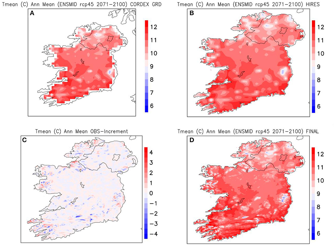
Figure 4. Illustration of the downscaling of EURO-CORDEX projections post quantile mapping, in this case for the annual mean of daily mean temperature from the mid-sensitivity ensemble under RCP4.5 for 2071–2100. The projected field on the EURO-CORDEX grid (A) is interpolated to the high-resolution observational grid (B). The adjustments derived from interpolating the historical observed field to the EURO-CORDEX grid and back again (C) are added to the field in (B) to give the final projected downscaled field in (D).

If T represents temperature or similar variable, and subscripts OBS and PROJ represent observations and projections, resp., the process can be described symbolically as:

$\begin{array}{l}{\text{T}}_{\text{PROJ}}(\text{CORDEX}\text{\_}\text{grid})\to {\text{T}}_{\text{PROJ}}(\text{hires}\text{\_}\text{grid})\\ [bylowtohi-resinterpolation]\\ {\text{T}}_{\text{OBS}\text{\_}\text{ORIG}}(\text{hires}\text{\_}\text{grid})\to {\text{T}}_{\text{OBS}}(\text{CORDEX}\text{\_}\text{grid})\\ [bystandardinterpolation]\\ {\text{T}}_{\text{OBS}}(\text{CORDEX}\text{\_}\text{grid})\to {\text{T}}_{\text{OBS}\text{\_}\text{DEG}}(\text{hires}\text{\_}\text{grid})\\ [bylowtohi-resinterpolation]\\ {\text{T}}_{\text{PROJ}\text{\_}\text{FINAL}}(\text{hires}\text{\_}\text{grid})={\text{T}}_{\text{PROJ}}(\text{hires}\text{\_}\text{grid})\\ +{\text{T}}_{\text{OBS}\text{\_}\text{ORIG}}(\text{hires}\text{\_}\text{grid})\\ -{\text{T}}_{\text{OBS}\text{\_}\text{DEG}}(\text{hires}\text{\_}\text{grid})\end{array}$

Here, T_{OBS_DEG}(hires_grid) represents the degraded observational field on the high-resolution grid. For a ratio variable like precipitation, the process is similar, only the final equation is multiplicative instead of additive:

$\begin{array}{l}{\text{P}}_{\text{PROJ}\text{\_}\text{FINAL}}(\text{hires}\text{\_}\text{grid})={\text{P}}_{\text{PROJ}}(\text{hires}\text{\_}\text{grid})\\ \times {\text{P}}_{\text{OBS}\text{\_}\text{ORIG}}(\text{hires}\text{\_}\text{grid})\\ /{\text{P}}_{\text{OBS}\text{\_}\text{DEG}}(\text{hires}\text{\_}\text{grid})\end{array}$

Figure 4D shows the result T_{PROJ_FINAL}(hires_grid) of such a process in the case of the annual mean field of daily-mean temperature from the mid-sensitivity ensemble under RCP4.5 for 2071–2100. Overall, Figures 4A–D illustrates the process described symbolically above. The large-scale features don't change between Figures 4A, D, but the process does provide extra local detail.

EURO-CORDEX fields based on histograms of occurrence frequency are downscaled slightly differently. They are interpolated from the EURO-CORDEX grid to the observational grid as above, but being frequency distributions, they lend themselves naturally to application of a second round of quantile mapping—this time not to correct biases based on historical performance, but simply to downscale. The role played by the historical simulations in “normal” quantile mapping is now played by T_{OBS_DEG}(hires_grid), i.e., the degraded observations after interpolation to the EURO-CORDEX grid and then back to the high-resolution grid again. Otherwise, the quantile-mapping algorithm runs much as before.

3. Results

3.1. Integrating the EURO-CORDEX and N&F projections

Once both the EURO-CORDEX and N&F ensembles are detrended, bias-corrected, and downscaled to the same high-resolution observational grid, how much relative weight should then be given to each individual (coarse-resolution) EURO-CORDEX simulation relative to each individual (high-resolution) N&F simulation when combining them into a single integrated ensemble? In practice this question is mostly moot, since the final projections for all the fields we have compared from both sets of ensembles are so similar as to be climatically identical. It makes almost no difference whether 80% weight is given to one and 20% to the other, or vice versa. For simplicity, then, the two sets of ensembles were combined into a single final set by giving equal weight to each individual ensemble member.

An example is shown in Figure 5, for the 99th percentile of daily precipitation amounts during autumn (Sept.-Nov.), from the middle-sensitivity ensemble under RCP4.5 for the period 2071–2100. Since autumn tends to be the wettest season in Ireland, these charts indicate what the wettest days during the wettest season would be like under that scenario. The top row (Figures 5A–C) shows the fields from the N&F ensemble, the EURO-CORDEX ensemble, and the combined ensemble, resp. The differences between the fields in Figures 5A, B are very small and difficult to see, so not surprisingly their combination in Figure 5C looks much the same again. The bottom row (Figures 5D–F) shows the ratios of the top row fields to the corresponding observed field from 1976 to 2005, and here the differences between the N&F ensemble (Figure 5D) and the EURO-CORDEX ensemble (Figure 5E) are more apparent, though still small. Their combination in Figure 5F shows a relatively simple pattern of rainy autumn days becoming wetter over most of the country by slightly more than 10% relative to the end of the 20th century.

FIGURE 5

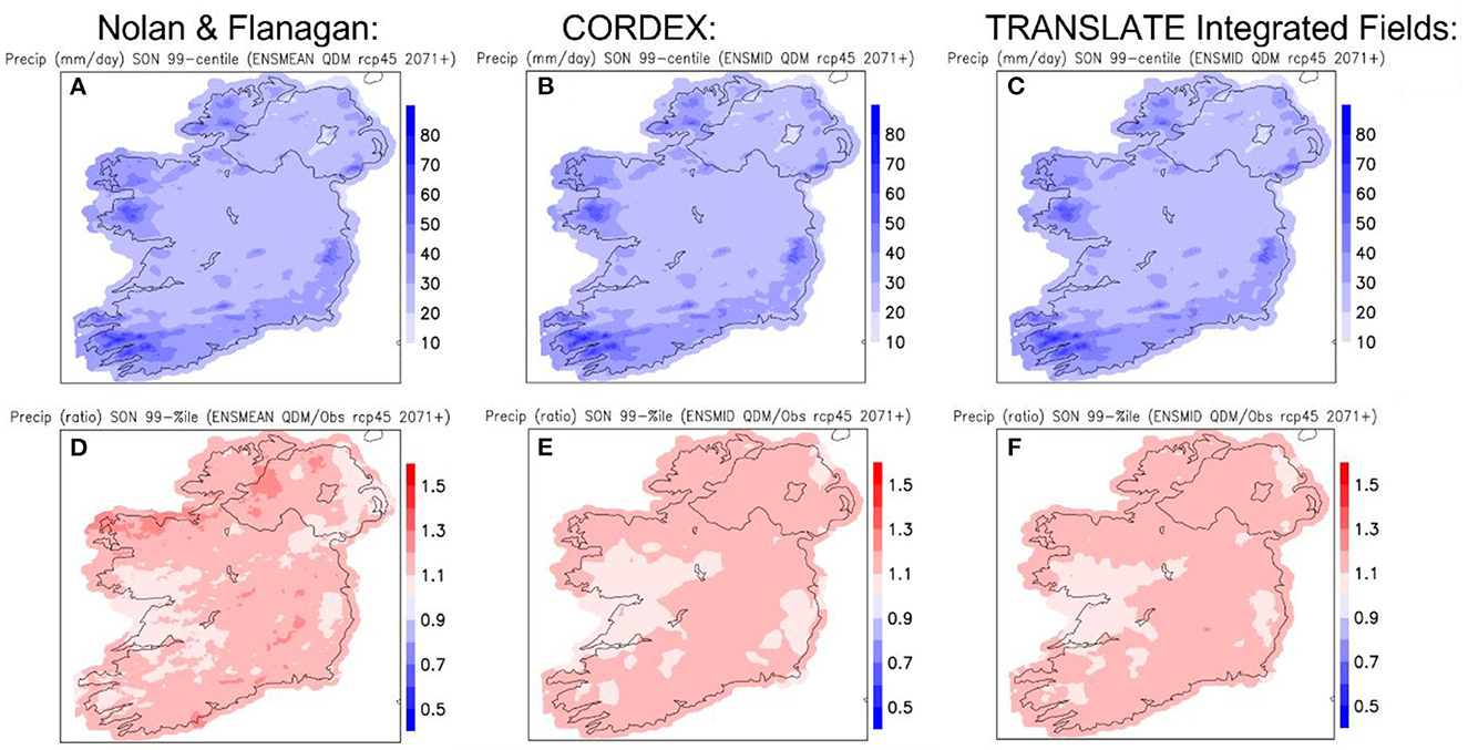
Figure 5. (A–C) Show the 99th percentile of daily precipitation amounts projected for the Sept.-Nov. season, by the mid-sensitivity ensembles under the RCP4.5 scenario for the period 2071–2100. (A) Shows the field from the Nolan and Flanagan (2020) ensemble; (B) from the EURO-CORDEX ensemble, while (C) is from the combination of the two, with equal weight assigned to each ensemble member. (D–F) Show the projected change signals as ratios of the fields in a-d relative to the corresponding observed field from 1976 to 2005, i.e., the (future projected value)/(historical observed value) at each grid-point.

3.2. Some illustrative sample results

3.2.1. Climate means

The projected end-century annual mean temperature fields under the three different emission scenarios and three different sensitivity ensembles are shown in Figure 6. Each map shows a lot of spatial detail, most of which corresponds to local elevations. All the main mountain ranges in Ireland can be easily identified. In each map, temperatures tend to be slightly cooler in the midlands and north, and slightly warmer around the coasts and toward the south, much as they are today. There is also a clear gradient across the nine maps shown, with temperatures increasing from left to right as the climate sensitivity increases, and from top to bottom as the emission scenarios increase from RCP2.6 to RCP8.5. Note that “absolute value” maps like this that have been bias-corrected are much more credible than raw RCP output, whose biases can be quite misleading.

FIGURE 6

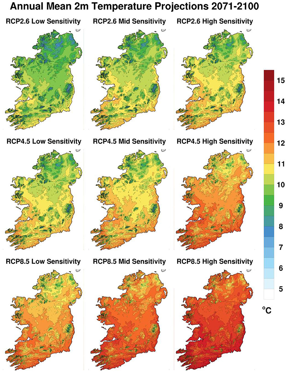
Figure 6. Projected annual mean surface temperature fields (°C) for the 2071–2100 period under the three different forcing scenarios and for the three different sensitivity ensembles.

The differences between each map in Figure 6 and the annual mean temperature during the reference period 1976–2005 are shown in Figure 7. Projected temperature changes relative to the reference period are all relatively uniform and smooth, with just a slight increasing gradient from west to east in each map. This gradient is likely due to the moderating influence of the Gulf Stream extension in the Atlantic acting most strongly on that part of Ireland closest to it. The inter-map differences are larger, with temperature changes increasing between maps from left to right as climate sensitivity increases, and from top to bottom as the emissions forcing increases. Of course, annual mean temperature is precisely the field that was used to define climate sensitivity, so the gradient from left to right in Figure 7 is pre-determined by that choice. Even so, it is apparent in Figure 7 that projected climates are more sensitive to the changes in RCP scenario than to the differences between the model responses (as measured by their climate sensitivity).

FIGURE 7

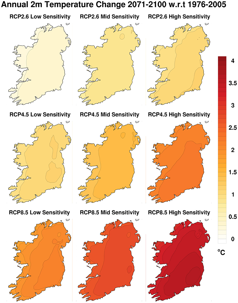
Figure 7. Differences between projected annual mean temperatures from the end-century period 2071–2100 and the reference period 1976–2005, under the forcing scenarios RCP2.6, RCP4.5, and RCP8.5, and the three different sensitivity ensembles.

The cross-section through Figure 1 for the annual mean of daily precipitation during the late- century 2071–2100 is shown in Figure 8. There is very little difference between any of the maps in Figure 8: they all show higher precipitation (up to 8 mm day⁻¹) over the higher elevations and along the western seaboard, with lowest values (2–3 mm day⁻¹) over the midlands and eastern regions. However, the difference between the 9 maps in Figure 8 become more apparent when shown in Figure 9 as percentage changes relative to observations during the reference period 1976–2005. Figure 9 shows that any precipitation increases tend to be largest (in percentage terms) in the midlands and east.

FIGURE 8

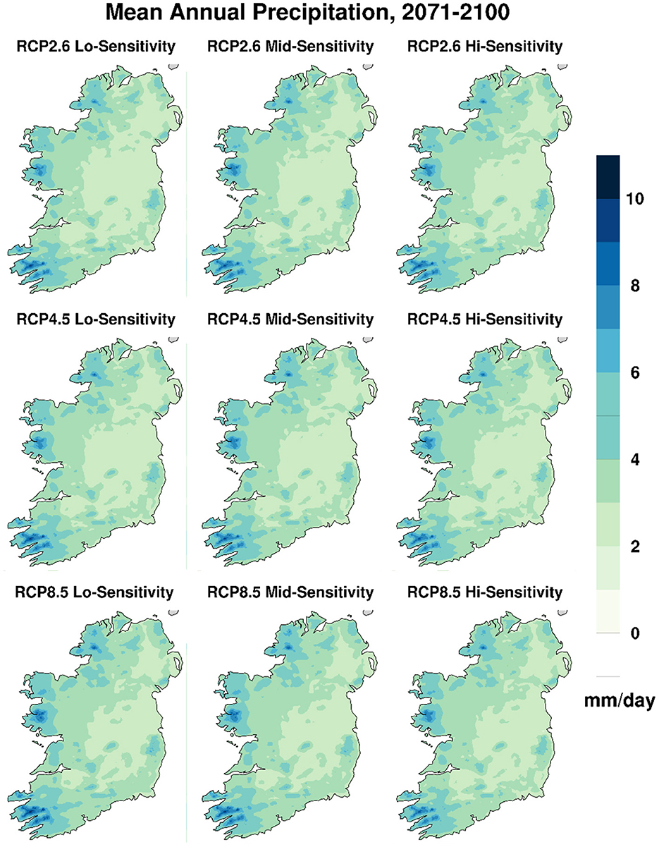
Figure 8. Projected annual mean daily precipitation fields (mm day⁻¹) for the 2071–2100 period under the three different forcing scenarios and for the three different sensitivity ensembles.

FIGURE 9

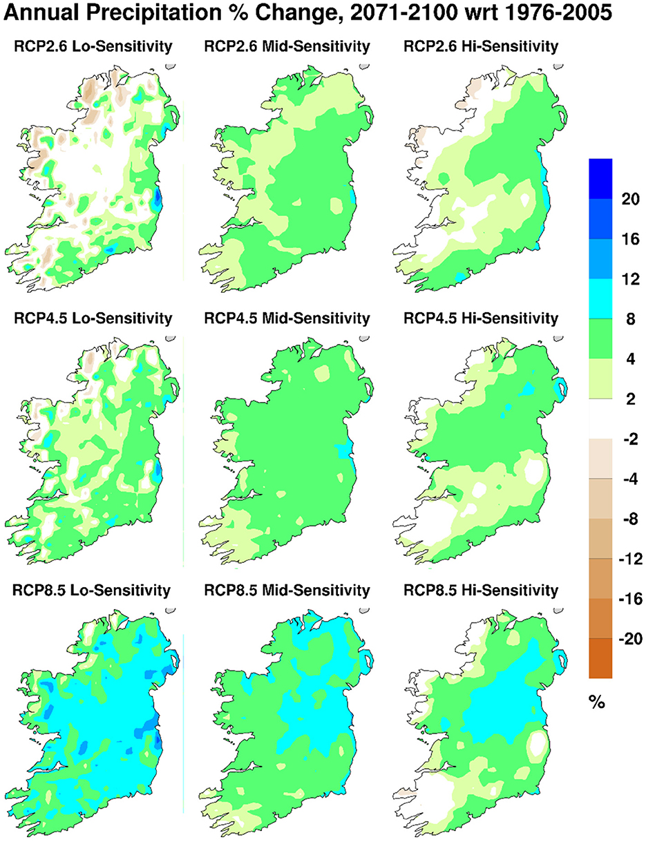
Figure 9. Differences between projected annual mean daily precipitation from the end-century period 2071–2100 and the reference period 1976–2005, under the forcing scenarios RCP2.6, RCP4.5, and RCP8.5, and the three different sensitivity ensembles.

Even the annual mean precipitation changes shown in Figure 9 mask significantly different behavior between the summer and winter seasons. Figure 10 shows projected precipitation changes during the end-century period as in Figure 9, but for the summer months June to August, while Figure 11 shows the corresponding change maps for the winter months December to February. Figures 9–11 all use the same contour intervals and the same color palette. The clear message is that summers are projected to become drier, while winters are projected to be wetter. Those patterns are amplified as the emission scenarios increase from RCP2.6 through RCP4.5 to RCP8.5. In contrast, the (temperature-based) climate sensitivity dimension does not show much variation, or any clear pattern. This is probably because there is only a weak relationship between temperature sensitivity and precipitation sensitivity over Ireland, where variable synoptic-scale circulation patterns can easily overcome the more direct Clausius-Clapeyron scaling between temperature and precipitation. See e.g., Houghton and O'Cinnéide (1976), Kiely (1999), or McCarthy et al. (2015) for evidence of how the Irish climate depends on large-scale circulation patterns in both the atmosphere and Atlantic ocean.

FIGURE 10

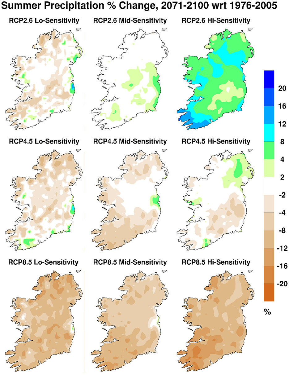
Figure 10. Percentage change in end-century projected daily precipitation, as in Figure 9, but for the summer months June to August.

FIGURE 11

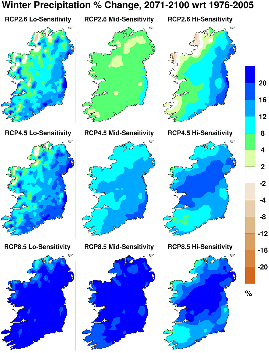
Figure 11. Percentage change in end-century projected daily precipitation, as in Figure 9, but for the winter months December to February.

Much as the annual mean precipitation projections (Figure 9) can mask large changes of opposite sign from summer and winter seasons (Figures 10, 11), so too can the individual ensemble-mean maps shown in Figures 9–11 mask large variability within each ensemble, as well as interannual variability within each ensemble member. This is illustrated in Supplementary Figure S4, which is analogous to Figure 9, but instead of the ensemble means, shows the ensemble range in each map, i.e., ensemble-maximum percentage change minus ensemble-minimum percentage change, for daily precipitation on each day of the year, then averaged over the annual cycle. The ranges are large, reflecting the fact that, e.g., if the projected ensemble minimum on each day is 1 mm day⁻¹ less than the observed amount while the ensemble maximum is 3 mm day⁻¹ more, at a point where the observed mean value is 4 mm day⁻¹, then the ensemble range of percentage change will be 100%. The sequence of Figure 8–11 and Supplementary Figures S4 shows how future precipitation projections can be deconstructed from a pattern of relative uniformity to reveal ever more variability as the projections are explored in more detail. This helps to distinguish those projected characteristics that are relatively robust from those that are more uncertain.

3.2.2. Projected frequency distributions

Frequency histograms were computed for each of the four main variables (T_mean, T_min, T_max, and precipitation), and for each 30-year climate instance (or ensemble member) of each projected climate. Temperature frequencies were binned in 1°C increments from −10 to 35°C, while precipitation frequencies were binned in increments of 2 mm day⁻¹ up to 80 mm day⁻¹.

Figure 12A shows annual and seasonal T_min histograms for 2071–2100 under RCP4.5 from the mid-sensitivity ensemble (solid curves) and for the observed reference period 1976–2005 (dashed curves), with local (grid-point) frequencies averaged over both the ensemble and the island of Ireland. The shading around each solid curve spans the range from minimum to maximum within the ensemble. The simplest interpretation of Figure 12A is that all the frequency curves retain much the same shape over time, but are shifted about 2°C to the right from the reference period to the end of the 21st century. The most dramatic changes thus occur near the tails. E.g., winter season T_min values of −5°C occurred with a frequency of about 0.02 (i.e., once every 50 winter-time days) during the reference period, as shown by the dashed blue curve in Figure 12A, but the frequency of similar cold nights by 2071–2100 under this scenario is projected to drop by a factor of 5 to about 0.004 (i.e., once every 250 winter days, only every 3 years or so). At the other extreme, summer nights with T_min values around 17°C are projected to occur up to 10 times more frequently than in the past. “Tropical nights” with T_min not falling below 20°C did not occur at all during the reference period but are projected to occur with a small but finite frequency in the future under this scenario.

FIGURE 12

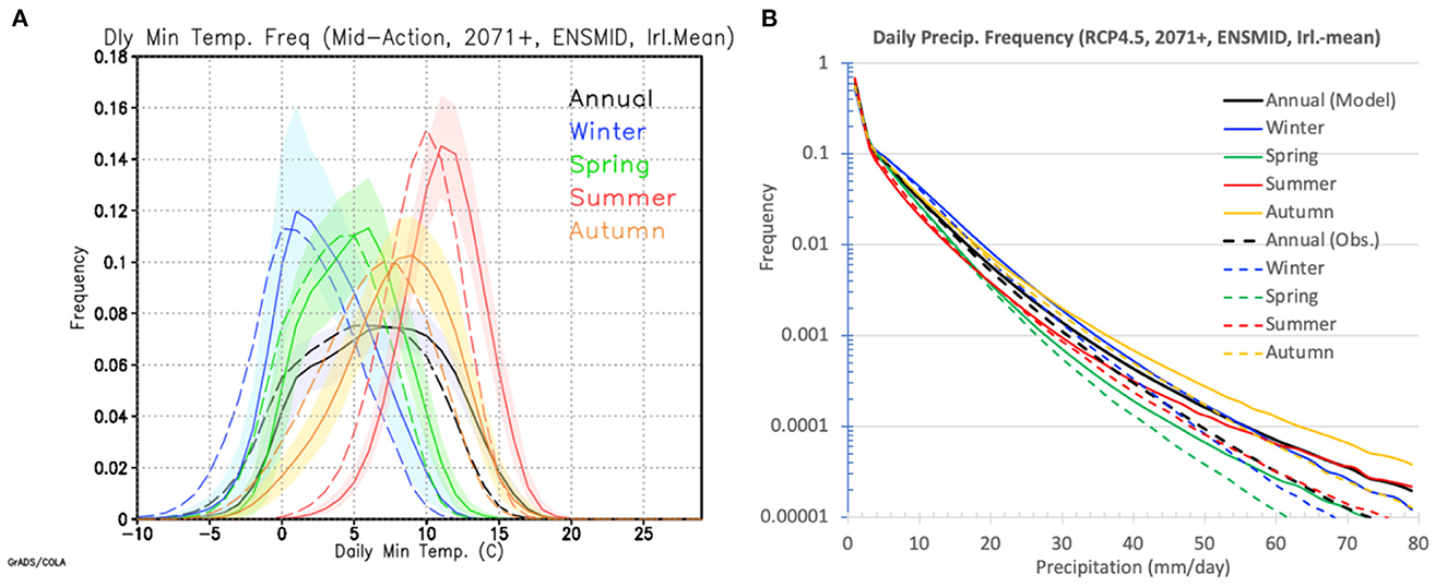
Figure 12. (A) Frequency distribution of projected daily minimum temperature (T_min) under the RCP45 (mid-range) forcing scenario for the end-of-century (2071–2100) from the mid- sensitivity ensemble, averaged over all Ireland, for each season and the annual cycle (solid curves). Shaded areas around each projected curve span the range from minimum to maximum value within the ensemble. The corresponding observed T_min values from the reference period 1976–2005 are shown as dashed curves. The temperature “bins” are 1°C wide; a frequency of 0.1 means that temperatures within that 1°C bin occur once every 10 days on average. (B) As in (A) except for daily precipitation, with frequency on a logarithmic scale, and for precipitation bins 2 mm day⁻¹ wide. No shading is shown as in (A) to avoid confusing the plot, but as the frequency decreases to 0.0001 (i.e., once in 10,000 days), the range of daily precipitation spans up to 50 mm day⁻¹ from ensemble minimum to ensemble maximum.

Precipitation is distributed differently to temperature, and so the precipitation frequency histograms in Figure 12B have a logarithmic y-axis. As in Figure 12A, the biggest differences between the past and projected future precipitation distributions are at the high-rainfall low-frequency tails. Thus, the wettest days are projected to get wetter in all seasons as well as for the year as a whole (all the solid curves at the tail of Figure 12B are to the right of the corresponding dashed curves). Spring-time rainfall events of 60 mm day⁻¹ that had a nominal occurrence frequency of 0.00001 (or a return period of 100,000 days) in the past (green dashed curve) are projected to occur about 3 times more often by the end of the century under this scenario (green solid curve).

The low frequencies of extreme events in Figure 12B are referred to as “nominal” above, because in reality they are relatively high-frequency localized events whose frequency value is reduced by the all-Ireland averaging. The curves in Figure 12 result from computing local frequencies and ensemble averaging first, and then doing all-Ireland averaging, instead of the other way round. This ordering doesn't really matter in the case of temperature (Figure 12A), since temperature anomalies tend to span wide areas, but in the case of precipitation (Figure 12B) it has the effect of expanding the sample size by several orders of magnitude before averaging it down again. Instead of ~20 ensemble members each with a single 30-year timeseries of daily data from which to compute event frequency, each ensemble member has 30 years of such data for each of about 2,000 (EURO-CORDEX) grid-points, or 30 years for each of hundreds of effectively independent locales where intense precipitation can occur. This sample multiplier effect is how return periods of up to 100,000 days (~275 years) can be plotted in Figure 12B. Even so, it is notable that most curves in Figure 12B have such smooth trajectories all the way down to the lowest frequencies and could reasonably be extrapolated further if desired. Plots like Figure 12B that are restricted to individual grid- points or small regions of just a few points only extend smoothly to frequencies of 0.001 (return periods of 3 years or so) before becoming noisy and non-monotonic (i.e., reporting isolated very wet events at the extreme tails of the distributions).

3.2.3. Temperature threshold-based projections

As mentioned in the Introduction, future climate ensembles were constructed from timeseries of 20-year periods centered on the year when the annual and global mean temperature from each underlying GCM used by TRANSLATE reached a specified threshold value above the pre-industrial mean from the same GCM. Three threshold values were considered, namely 1.5, 2.0, and 2.5°C. Table 2 shows the threshold- crossing dates for each RCP scenario for each of the CMIP5 GCM runs that were downscaled by either N&F or by EURO-CORDEX and further post-processed by TRANSLATE. Even the higher 2.5°C threshold was crossed by 16 different CMIP5 GCM simulations used by TRANSLATE, and most of those were further downscaled by multiple RCMs. This produced large ensemble sizes (>50 members) for each threshold climate. Each individual 20-year timeseries was then detrended, bias-corrected and further downscaled to the high-resolution observational grid, as was done for each of the 30-year timeseries underlying the different climate ensembles of Figure 1. One assumption behind assembling these large ensembles at different global warming levels is that the “path” to each level matters less than simply reaching and crossing that level. This assumes that the climate can adjust relatively quickly to a particular RCP forcing as time goes by. Experiments conducted by Ricke and Caldeira (2014) suggest that the timescale needed to adjust to an impulsive emission event is about 10 years, so the response time to more gradual forcing (as in the RCP scenarios) is presumably somewhat less than that.

TABLE 2

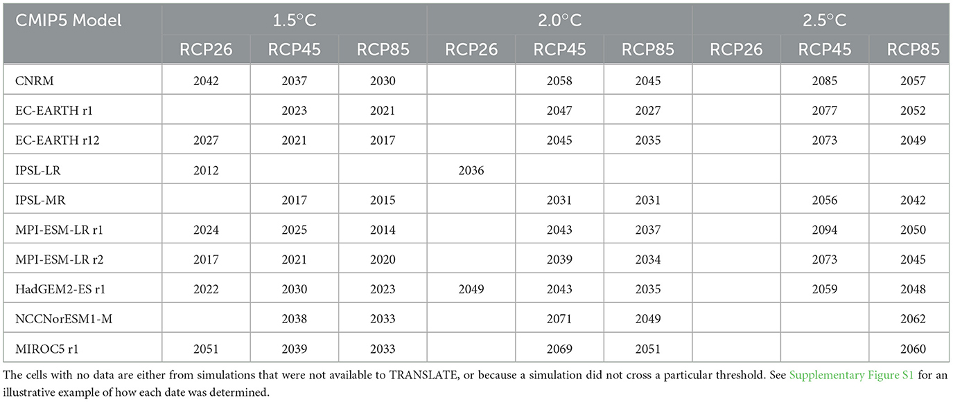
Table 2. The year at which the smoothed timeseries of global and annual mean surface temperature for the different CMIP5 GCM simulations listed crossed the 1.5, 2.0, and 2.5°C thresholds above their pre-industrial (1850–1900) mean.

While the temperature thresholds were computed relative to the pre-industrial period 1850–1900, only relatively sparse station observations are available from that period in Ireland. Such data as do exist were collected from hand-written records and transcribed to digital format by Mateus et al. (2020), and are available from the Met Éireann web-site.⁵ From this collection, 9 stations were selected for their geographical distribution around the country, and because each has relatively long and continuous observations of T_mean, T_min, and T_max from the pre-industrial period. Long-term mean values from these stations are shown in Supplementary Table S3, along with comparable data from the well-observed reference period 1976–2005 (The “pre-industrial” period is extended to 1914 or 1913 for a couple of stations for the sake of a longer continuous timeseries). For most stations, the 3 temperature variables increased from pre-industrial to modern times, on average by 0.51, 0.43, and 0.51°C for T_max, T_min, and T_mean, resp. However, there is large variation between stations, and even a couple of temperature decreases (shown in red font in Supplementary Table S3). The numbers are also sensitive to arbitrary choices, such as whether the Malin Head station data (from the northernmost tip of Ireland) are taken from 1885 to 1914, or from 1885 to 1900. Nevertheless, it seems reasonable to add an extra 0.5°C to any temperature change field that is computed relative to 1976–2005, in order to obtain an estimate of temperature change relative to 1850–1900. Moreover, this analysis was repeated using CRU temperature data over Ireland and obtained very similar results.

Figure 13 shows the T_mean changes (relative to 1976–2005) for each of the three threshold climates, and for the 10th percentile, mean, and 90th percentile of each threshold ensemble. As discussed above, a further 0.5°C should be added to each field in Figure 13 to approximate the projected changes relative to 1850–1900. In that case, the means of each ensemble (middle column in Figure 13) show changes over Ireland very close to, but perhaps slightly less than, the global mean change (i.e., 1.5, 2.0, and 2.5°C). As in the time- and scenario-dependent projections (e.g., Figure 7), the change fields are remarkably uniform and featureless, with relatively weak internal gradients across the country. Once again, the global change signal is very straightforwardly manifested in the projections over Ireland too. Of more significance, perhaps, is the relatively large spread within each ensemble, shown by the ~2.0°C differences between the 10th percentile fields (leftmost column of Figure 13) and the 90th percentile fields (rightmost column of Figure 13). This intra-ensemble spread reflects quite a large range of uncertainty that can be attributed mainly to differences between the models—both GCMs and RCMs. Analyses like this can be used to assign confidence levels to the projections, especially given the large ensemble sizes behind them. Thus, there is ~80% chance that temperature changes over Ireland (relative to 1976–2005) will be somewhere between the leftmost and rightmost columns of Figure 13 whenever any of the (global) temperature thresholds shown are reached.

FIGURE 13

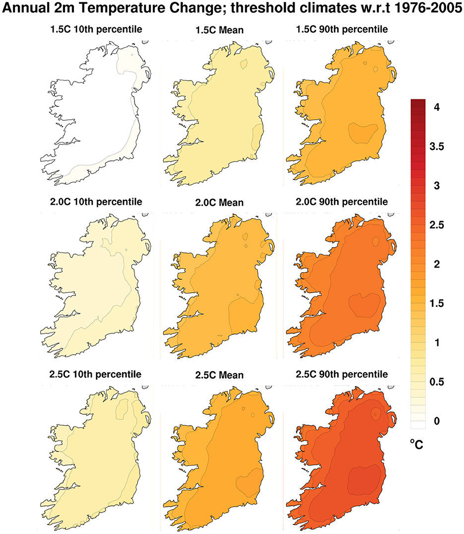
Figure 13. Projected annual daily mean temperature (T_mean) changes from the 1976–2005 reference period to a climate nominally 1.5, 2.0, and 2.5°C warmer than the pre-industrial period. The rows show the T_mean change fields for each threshold value, while the columns show the change fields for the 10th percentile, the mean, and the 90th percentile of each threshold ensemble.

3.2.4. Climate indices

A total of 27 standard climate indices are defined by the Expert Team on Climate Change Detection and Indices (ETCDDI).⁶ Most of the indices measure different aspects of climate extremes. They can all be easily computed from the (detrended and bias-corrected) 30-year timeseries files for each ensemble member in each ensemble shown in Figure 1, or from the 20-year timeseries for each ensemble member of each temperature threshold climate. TRANSLATE saves each such (reconstructed) timeseries so that any ETCDDI index, or indeed other custom indices (e.g., “growing season duration”) can be computed on demand. Typically, an index is computed for each year, then averaged over the duration of each timeseries; finally, the ensemble median is computed as the representative index value for that particular climate (e.g., each of the 27 sub-blocks in Figure 1). For reference, a regional breakdown of several such extreme climate indices using CMIP6 global model projections is provided by Almazroui et al. (2021). The changes in selected indices (TXx, TNn, R99p) relative to 1976–2005 are shown in Supplementary Figures S5–S7, as cross-sections through Figure 1 for the end century period 2071–2100.

4. Discussion and conclusions

A paradox of various national standards for future climate prections (e.g., UKCP18, CH2018, and KNMI'14 in the UK, Switzerland and the Netherlands, resp.) is just how different they all are from each other, each reflecting different national circumstances. This is also true of more recent projections for Central America by Tamayo et al. (2022). Nevertheless, it is clear from those projects that any standard future projection for Ireland should be based on high-resolution dynamical downscaling of global CMIP models. They should include a range of forcing scenarios to accommodate future emissions uncertainty, and a range of climate sensitivity responses to accommodate model uncertainty.

Ideally, future projections should be based on as large an ensemble as practically possible, with each ensemble member providing an independent climate instance of daily values of relevant variables for periods long enough to provide stable statistics (i.e., 20–30 years). Aggregated projections based on the modeled temperature crossing key thresholds are also worthwhile. The timeseries of each variable in each climate instance should be detrended, bias-corrected, and downscaled to the best possible grid-spacing to provide a stable climate reconstruction, which can then be queried for a wide range of statistics and climate indices. As shown in Section 2.4.3 and by Figure 4, statistical downscaling can add meaningful spatial information to climate projection fields that have coarser grids, just as dynamical downscaling by RCMs can provide more spatial detail than the low-resolution GCMs that drive them. Nevertheless, downscaling does not fundamentally alter or feedback on the climate change signal that is passed down from the coarser model grid.

An initial set of standardized climate projections for Ireland was produced, based on the dynamical downscaling work already done by N&F, and by the EURO-CORDEX project. These two sets of downscaled ensembles are nested in the same global CMIP5 models but are very different in the RCMs they use and in their native grid spacing. Given their different grid spacings and ensemble sizes, their post-processing by TRANSLATE to provide detrended, bias-corrected and fully downscaled output was done somewhat differently (Table 1). Nevertheless, the final projected output fields from both sets of ensembles tend to look remarkably similar (Figure 5). The future projected fields e.g., Figure 6 tend to include local details that reflect the main geographical features of Ireland, but the difference fields with respect to the reference 1976–2005 climate tend to be smooth and bland, reflecting the large-scale pattern of the underlying climate change signal (e.g., Figure 7). The similarity in the final future projections between the N&F fields and the EURO-CORDEX fields tends to serve as a cross-validation between them, increasing confidence in the validity of both.

Under the TRANSLATE project, initial standard projections for Ireland were built along the three separate axes of the cube shown in Figure 1, namely future forcing scenarios (as defined by the CMIP projects), future time periods, and climate sensitivity (as defined by the mean surface temperature response of the different ensemble members). Three further scenarios were based on 20-year time-periods around the 1.5, 2.0, and 2.5°C threshold warming levels as they are reached by simulations under different forcing scenarios. All the raw projected timeseries were detrended (using different methods for temperature and precipitation) and bias-corrected using quantile delta mapping, leading to completely reconstructed timeseries for each variable. The relatively coarse EURO-CORDEX fields were further interpolated and downscaled to the high-resolution observational grid by using the information lost as the observations themselves are interpolated to the coarse grid and back again. A second round of quantile mapping was applied to the EURO-CORDEX frequency fields, with the degraded observational field substituting for the historical simulation in the quantile mapping process.

An initial set of standardized climate projections for Ireland has already been produced by the TRANSLATE project using the principles and specific methods described above, and more complete results from these projections will become publicly available by summer 2023. Ultimately, our intent is to provide as complete and accessible quantitative information as practically possible about likely future climates in Ireland to meet the needs of those whose job is to plan and manage the national infrastructure out to the end of the 21st century.

Data availability statement

The raw data supporting the conclusions of this article will be made available by the authors, without undue reservation.

Author contributions

EO'B and PN are jointly responsible for the ideas behind this work and wrote the text. PN provided all the RCM output data. The RCM post-processing software was written and run by EO'B, in collaboration with PN. Both authors contributed to the article and approved the submitted version.

Funding

This work was funded by Met Éireann under the TRANSLATE project grant to the University of Galway.

Acknowledgments

The authors are grateful to the UK Met. Office for providing observational temperature data over Northern Ireland through their CEDA archive (https://data.ceda.ac.uk/badc/ukmo-metdb). We also benefitted from strategic oversight and direction provided by Peter Thorne and Bart van den Hurk.

Conflict of interest

The authors declare that the research was conducted in the absence of any commercial or financial relationships that could be construed as a potential conflict of interest.

Publisher's note

All claims expressed in this article are solely those of the authors and do not necessarily represent those of their affiliated organizations, or those of the publisher, the editors and the reviewers. Any product that may be evaluated in this article, or claim that may be made by its manufacturer, is not guaranteed or endorsed by the publisher.

Supplementary material

The Supplementary Material for this article can be found online at: https://www.frontiersin.org/articles/10.3389/fclim.2023.1166828/full#supplementary-material

Footnotes

1. ^E.g., the climate adaptation strategy for Co. Cork is available at https://www.corkcoco.ie/sites/default/files/2021-11/cork-county-council-climate-adaptation-strategy-2019-2024-pdf.pdf.

2. ^https://www.met.ie/science/translate

3. ^https://www.euro-cordex.net/

4. ^E.g., https://github.com/topics/quantile-delta-mapping.

5. ^https://www.met.ie/climate/available-data/long-term-data-sets

6. ^ETCI indices are listed at http://etccdi.pacificclimate.org/list_27_indices.shtml.

References

Almazroui, M., Saeed, F., Saeed, S., Ismail, M., Ehsan, M. A., Islam, M. N., et al. (2021). Projected changes in climate extremes using CMIP6 simulations over SREX regions. Earth Syst. Environ. 5, 481–497. doi: 10.1007/s41748-021-00250-5

CrossRef Full Text | Google Scholar

Cannon, A., Sobie, S., and Murdock, T. (2015). Bias correction of GCM precipitation by quantile mapping: how well do methods preserve changes in quantiles and extremes? J. Climate 28, 6938–6959. doi: 10.1175/JCLI-D-14-00754.1

CrossRef Full Text | Google Scholar

CH2018 (2018). NCCS (Pub.) 2018: CH2018 – Climate Scenarios for Switzerland. National Centre for Climate Services, Zurich. Available online at: https://www.nccs.admin.ch/nccs/en/home/data-and-media-library/data/ch2018-web-atlas.html (accessed February 09, 2023).

CH2018 Report (2018). CH2018 – Climate Scenarios for Switzerland, Technical Report. Eds. Fischer and Strassmann. Available online at: https://www.nccs.admin.ch/nccs/en/home/climate-change-and-impacts/swiss-climate-change-scenarios/technical-report.html (accessed February 09, 2022)

Chimani, B., Heinrich, G., Hofstätter, M., Kerschbaumer, M., Kienberger, S., Leuprecht, A., et al. (2016). ÖKS15–Klimaszenarien für Österreich. Daten, Methoden und Klimaanalyse; ZAMG: Wien, Österreich. Available online at: https://data.ccca.ac.at/dataset/endbericht-oks15-klimaszenarien-fur-osterreich-daten-methoden-klimaanalyse-v01 (accessed April 19, 2023).

Department of Communications, Climate Action and Environment, Government of Ireland. (2018). National Adaptation Framework: Planning for a Climate Resilient Ireland. Available online at: https://www.nwra.ie/wp-content/uploads/2020/05/national-adaptation-framework.pdf (accessed April 19, 2023).

Fauzi, F., Kuswanto, H., and Atok, R. M. (2020). Bias correction and statistical downscaling of earth system models using quantile delta mapping (QDM) and bias correction constructed analogues with quantile mapping reordering (BCCAQ). J. Phys.: Conf. Ser. 1538, 012050. doi: 10.1088/1742-6596/1538/1/012050

CrossRef Full Text | Google Scholar

Flanagan, J., and Nolan, P. (2020). Towards a Definitive Historical High-Resolution Climate Dataset for Ireland – Promoting Climate Research In Ireland. EPA Research Report 350. Available online at: https://www.epa.ie/pubs/reports/research/climate/researchreport350/ (accessed April 19, 2023).

Google Scholar

Flanagan, J., Nolan, P., McGrath, R., and Werner, C. (2019). Towards a definitive historical high-resolution climate dataset for Ireland–promoting climate research in Ireland. Adv. Sci. Res. 15, pp.263–276. doi: 10.5194/asr-15-263-2019

CrossRef Full Text | Google Scholar

Gutman, N. B. (1989). Statistical descriptors of climate. Bull. Am. Meteorol. Soc. 70, 602–607.

Google Scholar

Hanssen-Bauer, I., Førland, E., Haddeland, I., Hisdal, H., Lawrence, D., Mayer, S., et al. (2017). Climate in Norway 2100.

Google Scholar

Hollis, D., McCarthy, M., Kendon, M., Legg, T., and Simpson, I. (2018). HadUK-Grid Gridded and Regional Average Climate Observations for the UK. Centre for Environmental Data Analysis. UK Met. Office. Available online at: http://catalogue.ceda.ac.uk/uuid/4dc8450d889a491ebb20e724debe2dfb (accessed February 09 2023).

Houghton, J. G., and O'Cinnéide, M. S. (1976). Airflow Types and Rainfall in Ireland. Yearbook of the Association of Pacific Coast Geographers, Vol. 38, 33–48. Avaialble online at: https://www.jstor.org/stable/24041039 (accessed April 19, 2023).

Google Scholar

Kiely, G. (1999). Climate change in Ireland from precipitation and streamflow observations. Adv. Water Resour. 23, 141–151. doi: 10.1016/S0309-1708(99)00018-4

CrossRef Full Text | Google Scholar

Lenderink, G., van den Hurk, B., Klein Tank, A., van Oldenborgh, G., van Meijgaard, E., dev Vries, H., and Beersma, J. (2015). Preparing local climate change scenarios for the Netherlands using resampling of climate model output. Environ. Res. Lett. 9, 115008. doi: 10.1088/1748-9326/9/11/115008

CrossRef Full Text | Google Scholar

Lowe, J. A., Bernie, D., Bett, P., Bricheno, L., Brown, S., Calvert, D., et al. (2018). UKCP18 Science Overview Report. Available online at: https://www.metoffice.gov.uk/pub/data/weather/uk/ukcp18/science-reports/UKCP18-Overview-report.pdf (accessed February 09, 2023).

Google Scholar

Maraun, D. (2012). Nonstationarities of regional climate model biases in European seasonal mean temperature and precipitation sums. Geophys. Res. Lett. 39, L06706. doi: 10.1029/2012GL051210

CrossRef Full Text | Google Scholar

Maraun, D. (2013). Bias correction, quantile mapping, and downscaling: re- visiting the inflation issue. J. Clim. 26, 2137–2143. doi: 10.1175/JCLI-D-12-00821.1

CrossRef Full Text | Google Scholar

Mateus, C., Potito, A., and Curley, M. (2020). Reconstruction of a long-term historical daily maximum and minimum air temperature network dataset for Ireland (1831-1968). Geosci. Data J. 7, 102–115. doi: 10.1002/gdj3.92

CrossRef Full Text | Google Scholar

McCarthy, G. D., Gleeson, E., and Walsh, S. (2015). The influence of ocean variations on the climate of Ireland. Weather 70, 242–245. doi: 10.1002/wea.2543

CrossRef Full Text | Google Scholar

Murphy, J. M., Harris, G. R., Sexton, D. M. H., Kendon, E. J., Bett, P. E., Clark, R. T., et al. (2018). UKCP18 Land Projections: Science Report. Available online at: https://www.metoffice.gov.uk/pub/data/weather/uk/ukcp18/science-reports/UKCP18-Land-report.pdf (accessed February 09, 2023).

Google Scholar

Nilsen, I. B., Hanssen-Bauer, I., Dyrrdal, A. V., Hisdal, H., Lawrence, D., Haddeland, I., et al. (2022). From climate model output to actionable climate information in Norway. Front. Clim. 4, 866563. doi: 10.3389/fclim.2022.866563

CrossRef Full Text | Google Scholar

Nolan, P. (2015). Ensemble of Regional Climate Model Projections for Ireland. EPA Research Report 159, 88 p, Johnstown Castle, Ireland. Available online at: https://www.epa.ie/publications/research/climate-change/research-159-ensemble-of-regional-climate-model-projections-for-ireland.php (accessed April 19, 2023).

Google Scholar

Nolan, P., and Flanagan, J. (2020). High-Resolution Climate Projections for Ireland – A Multi-model Ensemble Approach. EPA Research Report 339, 81 p. Johnstown Castle, Ireland. Available online at: https://www.epa.ie/publications/research/climate-change/research-339-high-resolution-climate-projections-for-ireland-.php (accessed April 19, 2023).

Google Scholar

Nolan, P., O'Sullivan, J., and McGrath, R. (2017). Impacts of climate change on mid-twenty-first-century rainfall in Ireland: a high-resolution regional climate model ensemble approach. Int. J. Climatol. 37, 4347–4363. doi: 10.1002/joc.5091

CrossRef Full Text | Google Scholar

Ricke, K. L., and Caldeira, K. (2014). Maximum warming occurs about one decade after a carbon dioxide emission. Environ. Res. Lett. 9, 124002. doi: 10.1088/1748-9326/9/12/124002

CrossRef Full Text | Google Scholar

Rocheta, E., Evans, J. P., and Sharma, A. (2014). Assessing atmospheric bias correction for dynamical consistency using potential vorticity. Environ. Res. Lett. 9, 124010. doi: 10.1088/1748-9326/9/12/124010

CrossRef Full Text | Google Scholar

Ruosteenoja, K., and Jylhä, K. (2021). Projected climate change in Finland during the 21st century calculated from CMIP6 model simulations. Geophysica. 56, 39–69. Available online at: https://www.geophysica.fi/pdf/geophysica_2021_56_1_039_ruosteenoja.pdf (accessed April 19, 2023).

Google Scholar

Ruosteenoja, K., Jylhä, K., and Kamarainen, M. (2016). Climate projections for Finland under the RCP forcing scenarios. Geophysica 51, 17–50. Available online at: https://www.geophysica.fi/pdf/geophysica_2016_51_1-2_017_ruosteenoja.pdf (accessed April 19, 2023).

Google Scholar

Tamayo, J., Rodriguqz-Camino, E., Hernanz, A., and Covaleda, S. (2022). Downscaled climate change scenarios for Central America. Adv. Sci. Res. 19, 105–115. doi: 10.5194/asr-19-105-2022

CrossRef Full Text | Google Scholar

Taylor, K., Stouffer, R., and Meehl, G. (2012). An overview of CMIP5 and the experiment design. Bull. Amer. Meteorol. Soc. 93, 485–498. doi: 10.1175/BAMS-D-11-00094.1

PubMed Abstract | CrossRef Full Text | Google Scholar

The Royal Society (UK), National Academy of Sciences (USA). (2020). Climate Change: Evidence and Causes, Update 2020. Available online at: https://royalsociety.org/~/media/royal_society_content/policy/projects/climate-evidence-causes/climate-change-evidence-causes.pdf (accessed April 19, 2023).

Tiedtke, M. (1989). A comprehensive mass Flux scheme for cumulus parameterization in large-scale models. Mon. Wea. Rev. 117, 1779–1799.

Google Scholar

Van den Hurk, B., Siegmund, P., and Klein Tank, A., (Eds). (2014). KNMI'14: Climate Change Scenarios for the 21st Century – A Netherlands Perspective. KNMI scientific report WF 2014-01. Available online at: https://cdn.knmi.nl/knmi/pdf/bibliotheek/knmipubWR/WR2014-01.pdf (accessed April 19, 2023).

Google Scholar

Vautard, R., Gobiet, A., Sobolowski, S., Kjellstrom, E., Stegehuis, A., Watkiss, P., et al. (2014). The European climate under a 2°C global warming. Environ. Res. Lett. 9, 034006. doi: 10.1088/1748-9326/9/3/034006

CrossRef Full Text | Google Scholar

Walsh, S. (2016). Long-Term Rainfall Averages for Ireland, 1981–2010, Met Éireann, Dublin, Climatological Note No. 15. Available online at: http://hdl.handle.net/2262/76135 (accessed April 19, 2023).

Google Scholar

Walsh, S. (2017). Long-Term Temperature Averages for Ireland, 1981–2010, Met Éireann, Dublin, Climatological Note No. 16. Available online at: http://hdl.handle.net/2262/79901 (accessed April 19, 2023).

Google Scholar

Werner, C., Nolan, P., and Naughton, O. (2019). High-Resolution Gridded Datasets of Hydro-Climate Indices for Ireland. EPA Research Report 267. Available online at: https://www.epa.ie/publications/research/water/research-267.php (accessed April 19, 2023).

Google Scholar

Xavier, A., Martins, A., Rudke, A., de Morais, M., Martins, J., and Blain, G. (2022). Evaulation of Quantile Delta Mapping as a bias-correction method in maximum rainfall dataset from downscaled models in São Paulo state (Brazil). Int. J. Climatol. 42, 175–190. doi: 10.1002/joc.7238

CrossRef Full Text | Google Scholar