Fram strait—possible key to saving arctic ice

Arctic amplification caused by global warming is accelerating an unprecedented loss of Arctic sea ice due to thinning of multi-year sea ice and increased export through Fram Strait, which is the largest Arctic gateway for ice export. The transition to a thinner and younger Arctic ice cover has resulted in a steady surface albedo decline of 1.25–1.51% per decade, weakening the radiative cooling effect of sea ice by 0.04–0.05 W m^–² per decade. The Fram Strait ice export (FSIE) is a major sink in the Arctic ice mass balance, accounting for approximately 14% of the annual sea ice volume loss. As the ice becomes thinner, it drifts faster, leading to enhanced ice export. The annual and summer FSIE have increased by about 6% and 11% per decade, respectively, further accelerating Arctic sea ice decline. Surface Albedo Modification (SAM) has been considered among variety of climate intervention solutions to slow down the transition of the Arctic into a seasonally ice-free ocean by mid-century, in concert with the greenhouse emissions mitigation efforts. Using climate model simulations, we evaluate the impacts of SAM application on the Arctic radiation budget and ice cover in two deployment scenarios: Arctic-wide and regional in Fram Strait. We model such an increase in sea ice albedo as a perturbation to the present-day climate state. Our results show that enhancing the surface albedo by up to 20% Arctic-wide during summer reduces the absorbed radiation at the surface by 11.16 W/m² and increases outgoing radiation at the top of the atmosphere by 10.70 W/m². This results in surface cooling of –1.33°C and recovers approximately 10% of the present-day Arctic sea ice radiative cooling power. These findings suggest that large-scale surface albedo modification could offset Arctic warming and contribute measurably to global cooling. The regional targeted deployment in Fram Strait yields more spatially limited but dynamically significant responses. SAM in Fram Strait enhances surface albedo both locally and in adjacent regions (Barents, Kara Sea) through advection of thicker, more reflective ice. The resulting radiative cooling alters atmospheric circulation, strengthening the low-pressure system over the Barents–Kara sector and triggering a negative Arctic Dipole pattern. This reduces sea-ice export by 2.4% through Fram Strait via weakening the Transpolar Drift in addition to the local thickening and slowing of the ice in the FS region, supporting ice retention within the Arctic basin. Furthermore, the modified atmospheric circulation induces dynamically driven nonlocal ice growth in areas of Central Arctic which persist year-round. These results highlight the potential of Fram Strait albedo enhancement to support multi-year ice recovery and reduce its loss via the Fram Strait. While basin-wide SAM offers the greatest potential benefits, it remains logistically challenging and carries higher risks of unintended consequences. Targeted regional interventions—such as in the Fram Strait and marginal seas (Barents, Kara, and Beaufort)—present a more feasible and cost-effective alternative, with lower risks and the potential to induce basin-wide responses through coupled atmosphere–ice–ocean interactions. These regions are dynamically linked to major circulation centers, including the Barents–Kara Low and Beaufort High, making them promising leverage points for intervention. A strategy for Arctic climate intervention, where a coordinated, regionally targeted, and seasonally adaptive deployment—combining summer albedo enhancement with winter ice thickening—may offer the greatest potential to stabilize Arctic sea ice while minimizing risks.

1 Introduction

The Arctic is warming at twice the rate as the rest of the planet, accelerating sea ice loss (Richter-Menge et al., 2019). Sea ice thinning over marginal sea ice areas causes near-surface warming of 1 °C per decade in winter, increasing the Arctic amplification factor by 37% (Lang et al., 2016). Transition of the Arctic into a seasonally ice-free ocean (Overland and Wang, 2013) will increase air temperatures and cause precipitation phase changes (Landrum and Holland, 2020) that will affect summer precipitation in Europe, the Mediterranean, and East Asia (Vihma, 2014; Screen et al., 2011) and increase droughts in California (Cvijanovic et al., 2017). Fram Strait sea ice transport is tightly coupled to atmospheric dynamics and ocean circulation in the North Atlantic–European sector, and improved understanding of these linkages is critical for predicting abrupt shifts in the Atlantic Meridional Overturning Circulation and European climate extremes (Ionita et al., 2016).

Accounting for more than 90% of the total Arctic sea ice export (Haine et al., 2015) and approximately 14% of the annual Arctic sea ice volume loss (Spreen et al., 2020), the Fram Strait ice export (FSIE) represents a major sink in the Arctic ice mass budget. Since 1979, sea ice area export through the Strait has increased by 6% annually and 11% per decade in spring, further accelerating Arctic ice loss (Halvorsen et al., 2015; Smedsrud et al., 2011, 2017). The dominant dynamical driver of the FSIE is the wind-driven Transpolar Drift, a component of the large-scale Arctic sea ice circulation, which transports thinner sea ice from the eastern Siberian shelf across the pole toward the Fram Strait (FS). The southward sea ice flow through the strait is controlled by the across-strait sea level pressure gradient (Lang et al., 2016; Serreze and Barrett, 2011; Spall, 2019), which is part of the second dominant mode of atmospheric variability in the Arctic (Tsukernik et al., 2009; Wu and Johnson, 2007; Vihma et al., 2012). This mode features an east–west dipole with a low-pressure anomaly center in the Barents Sea (BS) and Kara Sea (KS) and a high-pressure anomaly in the Canadian Archipelago. Intensifying or diminishing the negative anomaly in BS enhances or weakens northerly winds through the FS, consequently increasing or reducing the exported sea ice (Tsukernik et al., 2009). Long-term observational records (1948–2014) confirm a strong linkage between the Fram Strait export anomalies and the Arctic dipole (AD) (Smedsrud et al., 2017). The recent low Arctic ice outflow extreme in 2018 was attributed to a persistent east–west dipole-like atmospheric pattern (Sumata et al., 2022).

Analysis of sea ice drifts derived from satellite observations shows that the winter anomaly of sea ice export is correlated positively with the winter Arctic Oscillation (AO) index and negatively with the following September sea ice extent (Williams et al., 2016). Such correlations are weak when the sea ice cover is strong enough to resist the anomalous wind forcing caused by different phases of the AO. To maintain a fully ice-covered Arctic in winter, there needs to be an enhanced first-year ice that is thick enough to survive the following summer melt season, compensating for the net deficit in the sea ice area budget (Williams et al., 2016).

Arctic surface albedo has declined steadily by approximately 1.25–1.51% per decade since the early 1980s, as observed from satellite data (Zhang et al., 2019). This decline is primarily driven by sea ice thinning and shrinking, the expansion of darker open water, and the retreat of seasonal snow cover—processes that intensify surface warming through the ice–albedo feedback (Marcianesi et al., 2021). As a consequence, the radiative cooling effect of Arctic sea ice has weakened by 0.04–0.05 W m⁻² per decade, amounting to an overall reduction of approximately 24% since 1980 (Duspayev et al., 2024). The positive albedo amplification effect (Previdi and Simmonds, 2021), whereby small initial losses in ice or snow cover lower surface reflectivity, increase solar energy absorption, and accelerate further melt, amplifies Arctic warming at a rate more than twice the global average (Dai, 2021). Model-based analyses (Thackeray and Hall, 2019; see Figure 1 in their study) and recent observational estimates (Rantanen et al., 2022) further show that, regionally, the Barents Sea and Kara Sea exhibit the strongest albedo amplification effect, owing to large seasonal ice losses. Recent observations confirm that the Barents Sea, in particular, has become a major hotspot of Arctic warming, with winter surface temperatures rising nearly four times faster than the global average, driven by sea ice retreat and reduced albedo (Isaksen et al., 2022; Rantanen et al., 2022).

Figure 1

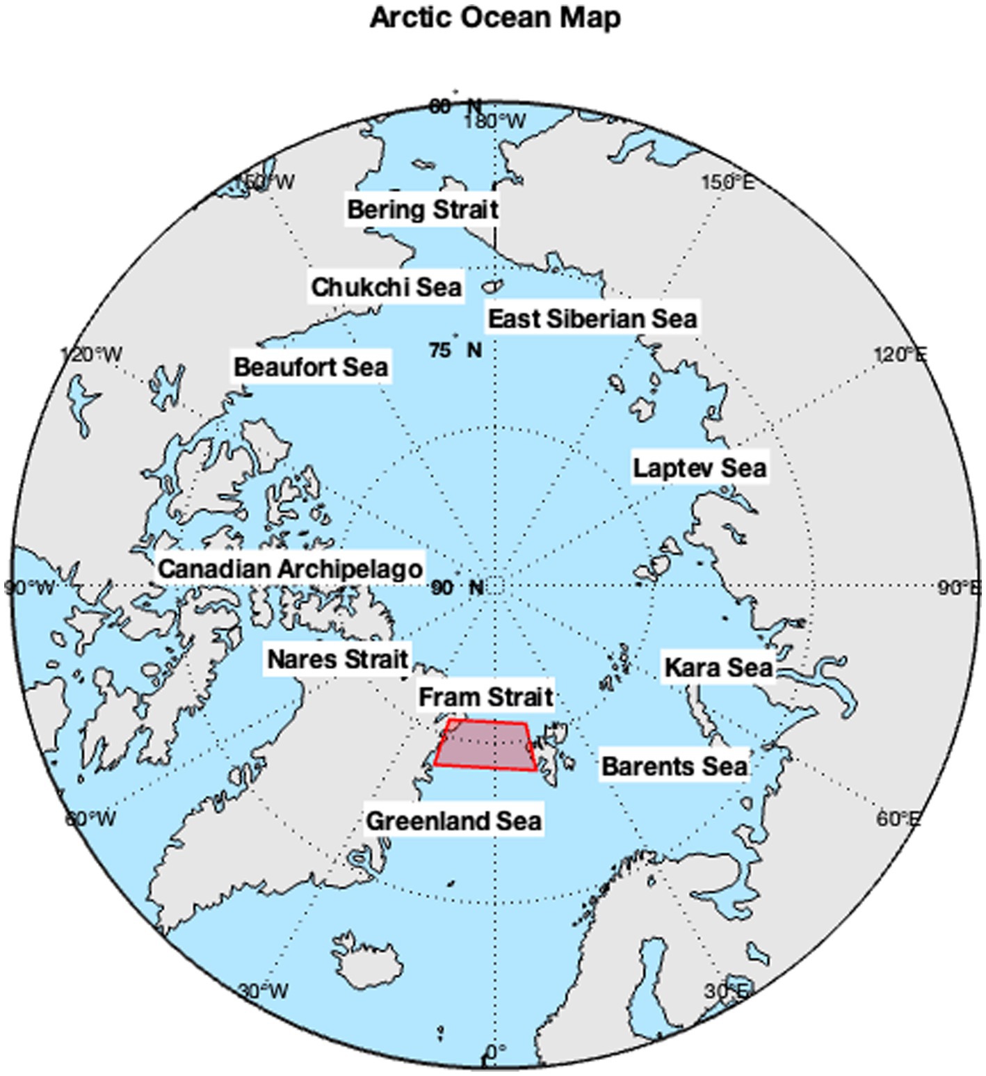
Figure 1. Arctic Ocean map. The Fram Strait study region is outlined in red.

The main objective of this study is to assess the impact and effectiveness of the surface albedo modification (SAM) strategy as a potential Arctic climate intervention. We examine two deployment scenarios by using climate model simulations: (i) a large-scale, Arctic-wide application and (ii) a localized, regional implementation in the Fram Strait (FS). Given the critical role of the FS in regulating Arctic sea ice mass balance, targeting this region offers a strategic opportunity to optimize the SAM benefits for sea ice recovery. The primary goal of the SAM application in the FS is to mitigate the accelerated ice mass loss observed in recent decades by enhancing ice thickness and reducing ice export, thereby providing a regulatory mechanism to control Arctic ice mass loss through the FS. Furthermore, we hypothesize that localized albedo enhancement in the Fram Strait triggers non-local atmospheric and sea ice responses, thereby amplifying its influence across the Arctic basin. We investigate whether the impact of increasing sea ice albedo (Field et al., 2018) over the FS can be a key lever in restoring Arctic sea ice and slowing down its export from the Arctic.

Details of the climate modeling and simulations are provided in Section 2 (Methods). Section 3 (Results) presents the analysis of radiative effects, atmospheric dynamics, and sea ice responses. The underlying mechanisms and potential practical applications are discussed in Section 4 (Discussion) and Section 5 (Conclusion).

2 Methods

We use the National Center for Atmospheric Research Community Earth System Model (CESM) version 1.2, which incorporates interactive atmospheric (CAM4), sea ice (CICE4), ocean (POP2), and land (CLM4) components. To establish a present-day baseline for the albedo perturbation experiments, we employ a scenario with climatological 2000s greenhouse gases (GHG) and aerosol forcing. Specifics on modeling the surface albedo modification (Field et al., 2018) adopted for this study are described in the Supplementary material S1. However, we briefly mention the salient points here. Modeling the sea ice albedo perturbation using the “delta Eddington”(DE) shortwave parameterization in the sea ice model component CICE of CESM (Briegleb and Light, 2007) involves assigning to the albedo perturbation area different physical properties of the snow layer (see Supplementary material for more details), resulting in a different albedo than the rest of the sea ice cover. We design the perturbation experiment with the underlying assumption that whenever sea ice is present in the treated region, the sea ice albedo perturbation will apply. Thus, during the melt season, as sea ice retreats and ocean waters are uncovered, the sea ice albedo perturbation diminishes. The climate system exhibits strong internal natural variability, which can result in large-scale changes over short time periods. In the Arctic, the dominant mode of variability is the AO, defined as the first empirical orthogonal function mode of the winter surface pressure pattern in the Northern Hemisphere. It is characterized by Polar low-pressure and high-pressure centers in the mid-latitudes (Thompson and Wallace, 2000).

Three numerical experiments were conducted to assess the impact of surface albedo modification (SAM): a control simulation (CONTROL) with no albedo modification, a localized perturbation in the Fram Strait (FRAM), and a large-scale Arctic-wide perturbation (GLOBAL). The Fram Strait region where the albedo perturbation is applied (78.05–80.87°N, 18.75–12.5°E) covers an area of 151,200 km² (see Figure 1, outlined with red lines).

To address possible ranges of climate variability, for each type of numerical experiment, we run an ensemble of three members initialized at each phase of the AO (i.e., the positive, negative, and neutral phases). Ideally, this initialization approach sets the ensemble members’ AO variability out of phase with each other, and when creating their ensemble mean, they would cancel and thus eliminate or reduce the signal of the dominant AO pattern and reveal the effect of the otherwise not-so-strong Fram albedo perturbation. Initial states are selected from the last decade of an 80-year spin-up control simulation. All simulations are fully coupled present-day climate simulations, evolving continuously along their own trajectory. They are initialized in the year 2000 and integrated forward for 80 years. The GHG forcing remains constant, using the GHG climatology for the 2000s. This represents a present-day or future mitigation scenario in which we contain the future GHG forcing to the 2000 GHG forcing.

Our primary focus in this study is on the FRAM experiment results; however, where applicable, we also use results from the GLOBAL experiment to provide additional insights. The analysis of the results is presented in terms of ensemble mean characteristics. For each of the major experiments (CONTROL, GLOBAL, and FRAM), ensemble mean time series are generated by averaging the three-member ensembles initialized from the neutral, negative, and positive AO phases. The ensemble spread is defined as the range between the minimum and maximum values of the ensemble members. Annual and seasonal climatologies are calculated for the period 2001–2080, excluding the first year of integration to reduce the impact of the initial adjustment. The statistical significance of the differences between the ensemble mean seasonal climatologies of the experiments is evaluated using a two-tailed t-test at the 90% and 95% confidence level.

We use the atmospheric model output to calculate the radiation balance at the surface (Net SRF) and at the top of the atmospheric model (Net TOM), area-averaged north of 70°N. All radiation budget components are in W/m², and the positive direction is downward.

The net surface radiation balance is derived as follows:

$\begin{array}{ll}\mathrm{Net}\mathrm{SRF}=\mathrm{Net}{\mathrm{SW}}_{\mathrm{SRF}}-\mathrm{Net}{\mathrm{LW}}_{\mathrm{SRF}}-\mathrm{LH}-\mathrm{SH}& (1)\end{array}$

where,

Net SW_SRF = SWD_SRF − SWU_SRF is the net shortwave radiation at the surface; SWD _SRF is the− shortwave down flux at the surface; and SWU_SRF is the shortwave up flux at the surface; Net LW_SRF = LWU_SRF − LWD_SRF is the net longwave radiation at the surface; LWU_SRF is the longwave up flux at the surface; LWD_SRF is the longwave down flux at the surface; LH is the latent heat flux at the surface; and SH is the sensible turbulent heat flux at the surface.

The top of the model (TOM) net radiation is calculated as the residual of the net shortwave radiation − net longwave radiation at the top level of the atmospheric model:

$\begin{array}{ll}\mathrm{Net}\mathrm{TOM}=\mathrm{Net}{\mathrm{SW}}_{\mathrm{TOM}}-\mathrm{Net}{\mathrm{LW}}_{\mathrm{TOM}}& (2)\end{array}$

where,

Net SW_TOM = SWD_TOM − SWU_TOM is the shortwave flux at the top of the model; SWD_TOM is the shortwave down flux at the top of the model; SWU_TOM is the shortwave up flux at the top of the model; Net LW_TOM = LWU_TOM − LWD_TOM is the net longwave flux at the top of the model; LWU_TOM is the longwave up flux at the top of the model; and LWD_TOM is the longwave down flux at the top of the model.

3 Results

Using atmospheric and sea ice model outputs from our fully coupled climate model simulations, we assessed the impacts of surface albedo modification under two scenario experiments: GLOBAL, representing Arctic-wide application, and FRAM, representing localized application in the Fram Strait region. Both cases were evaluated in relation to the CONTROL simulation, which did not include surface albedo modification. We first quantify the effects of albedo perturbations on the surface and top-of-atmosphere radiation budgets. We then examine the resulting changes in atmospheric dynamics and the subsequent response of sea ice. Finally, we evaluate the overall efficacy of the albedo intervention in achieving its intended objectives.

3.1 Albedo perturbation

The strongest impact of an albedo perturbation occurs during the daylight season, when insolation is at its maximum. Figure 2 shows the summer mean spatial distributions of the applied surface albedo perturbations, derived as ensemble mean differences between the albedo-modified cases (GLOBAL and FRAM) and the baseline CONTROL, averaged over the 80-year integration. These increases are statistically significant at greater than the 95% confidence interval, as tested through a t-test. In the GLOBAL case (Figure 3a), the albedo increases basin-wide with the strongest impact >25% in the marginal ice zone and approximately 15–20% in the Central Arctic. Averaged over the entire Arctic basin (North of 70°N), the increase is 13.4% (Table 1, ALBEDO_SRF). At the top of the atmospheric model, the albedo increases by 3.4% (Table 1, ALBEDO_TOM). This is comparable to the 4% Arctic albedo reduction observed in satellite records in the period 1979–2011 (Pistone et al., 2014). The summer surface albedo in the FRAM case (Figure 3b) shows an increase of approximately 15–20% over the treated FS region. There are significant albedo increases of 5–10% over Svalbard, the area to its east, and parts of BS and KS, which are outside the treatment region.

Figure 2

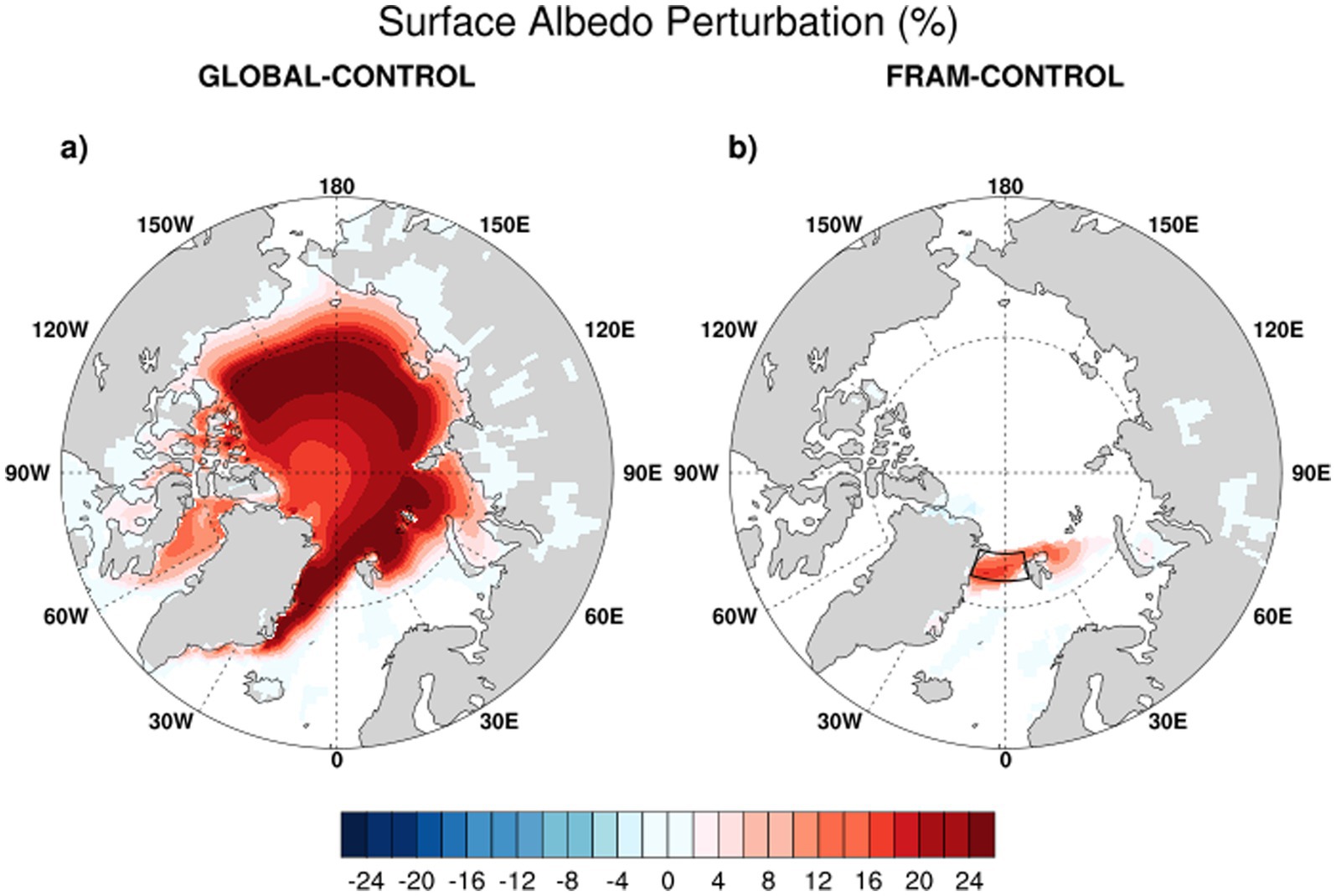
Figure 2. Summer (July–August–September, JAS) maps of the surface albedo perturbations (%) derived as ensemble mean differences averaged over the integration period 2001–2080 in two surface albedo modification cases (GLOBAL and FRAM) referred to the CONTROL case: (a) GLOBAL–CONTROL and (b) FRAM–CONTROL. The significance of the differences is evaluated using a two-tailed t-test. Only the statistically significant differences at a 95% confidence level are shown in color. The Fram Strait treatment region is outlined with black lines.

Figure 3

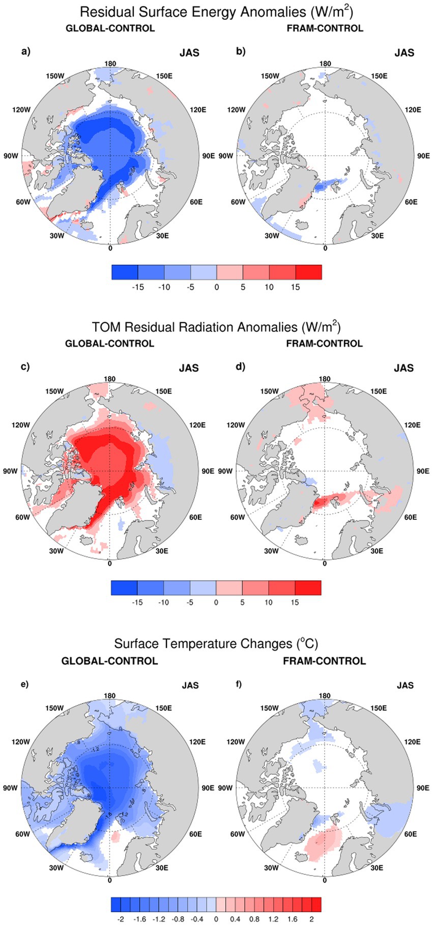
Figure 3. Arctic summer (July–August–September, JAS) radiation balance changes derived as ensemble mean differences averaged over the integration period 2001–2080 in the two surface albedo modification cases (FRAM and GLOBAL) referred to CONTROL case: (a) GLOBAL–CONTROL residual (net) surface radiation flux differences (W/m²); (b) FRAM–CONTROL residual (net) surface radiation flux differences (W/m²); (c) GLOBAL–CONTROL residual Top of the Model (TOM) radiation flux differences (W/m²); (d) FRAM–CONTROL residual TOM radiation flux differences (W/m²); (e) GLOBAL–CONTROL surface temperature (TS) differences (°C); and (f) FRAM-CONTROL surface temperature (TS) differences (°C). The significance of the differences is evaluated using a two-tailed t-test. Only the statistically significant differences at a 90% confidence level are shown in color; the insignificant values are masked out.

Table 1

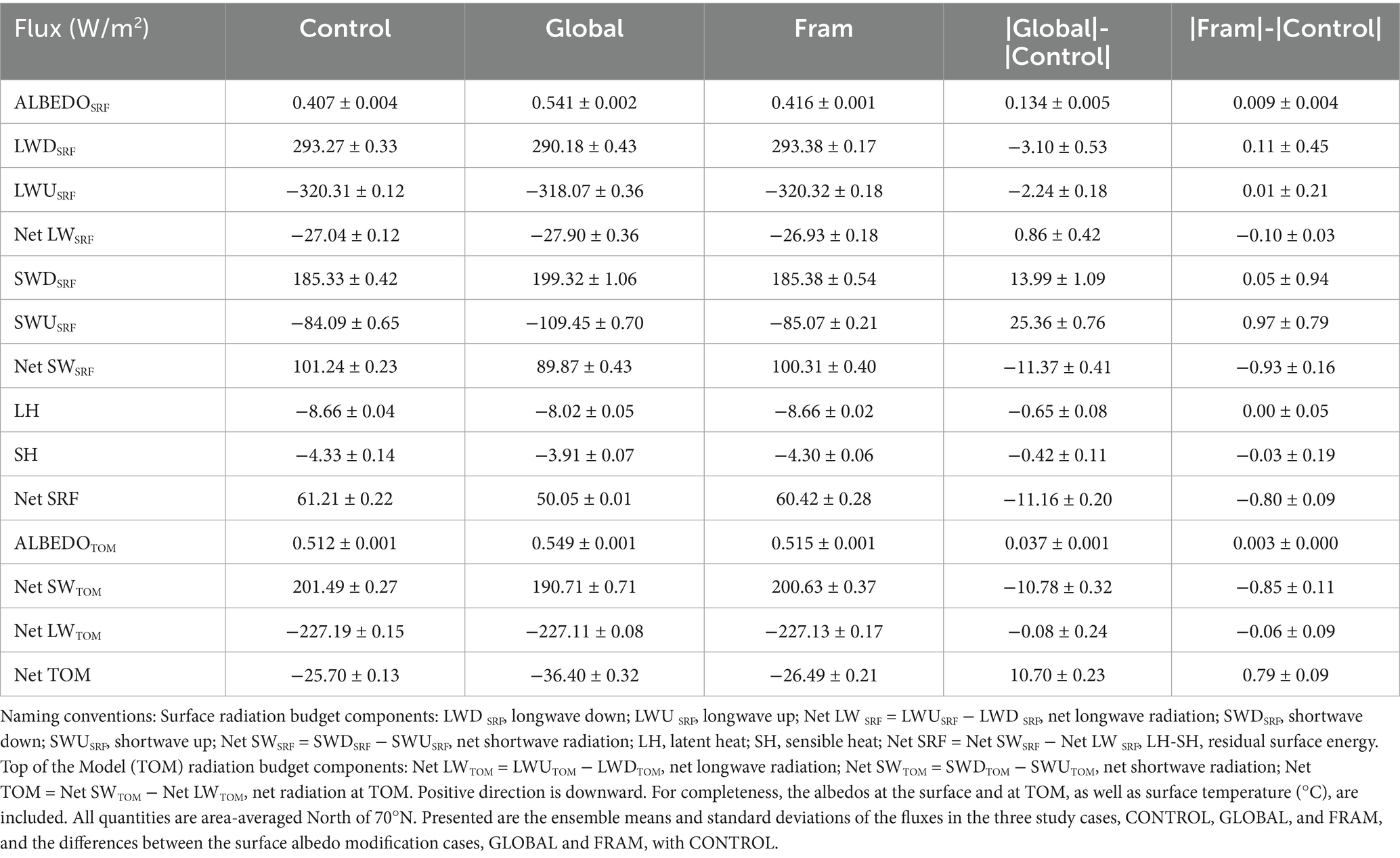
Table 1. Summer (JJA) Arctic Radiation Budget fluxes (W/m²) at the surface (SRF) and at the Top of the Model (TOM) Positive direction is downward.

3.2 Radiation balance changes

The objective of perturbing the surface albedo is to change the balance of the surface radiation fluxes to reduce the absorbed heat by the surface. Such albedo perturbations have a direct impact only during the daylight time of the year (March–September in the polar areas). Once applied, the surface radiation fluxes respond immediately. The summer (JAS) mean climatology maps of the Arctic residual (net) surface radiation flux changes (differences between GLOBAL/FRAM and CONTROL ensembles means) show an Arctic-wide reduction in the GLOBAL case (Figure 3a) over the FS region in the FRAM case (Figure 3b), indicating reduced absorption of the solar radiation at the surface. The radiation changes at the surface propagate to the top of the atmospheric model (TOM) and are shown as an increase in the residual TOM radiation flux basin-wide in the GLOBAL case (Figure 3c) and over both FS and Bering Strait regions in the FRAM case (Figure 3d), implying an increased amount of outgoing radiation to space. These radiation balance changes result in cooling surface temperature anomalies. In the GLOBAL case, the Arctic cools basin-wide, with maximum cooling of −2 °C north of Greenland (Figure 3e). The cooling anomalies in the FRAM case are smaller, at approximately −0.2 °C, and found over the FS and also KS, the Bering Sea, and parts of the Beaufort Gyre region (Figure 3f).

To further quantify changes in the radiation budget, we examine the mean budget components averaged over the Arctic region north of 70°N (Table 1). In the GLOBAL case, the net surface radiation decreases by 11.16 W/m² in summer (Table 1, Net SRF), while the outgoing radiation at the top of the atmosphere increases, reducing the radiative forcing by 10.70 W/m² during the same season (Table 1, Net TOA). On an annual basis, these changes are −3.57 W/m² and +2.14 W/m², respectively. The latter corresponds to a 0.07 W/m² reduction on the planetary-scale—approximately 10% of the current total Arctic sea ice radiative cooling effect estimated at 0.71 W/m² (Pistone et al., 2019; Duspayev et al., 2024).

Similar direction changes, but with smaller magnitude −0.8 W/m² reduction of the net surface radiation and 0.79 W/m² increase of the TOM outgoing radiation—are found in the FRAM case as well. In both cases, the largest contributor to the net surface radiation flux (Table 1, Net SRF) change is the outgoing shortwave radiation from the surface (Table 1, SWU_SRF). The increased summer net TOM radiation (Table 1, Net TOM) is due to the decreased net shortwave (Table 1, Net SW_TOM). The rest of the radiation budget components (Table 1, LH, SH, Net LW_SRF), as well as the outgoing longwave at TOM (Table 1, Net LW_TOM), are reduced with the albedo perturbation.

Next, we assess the cooling impact of the SAM applications in the Arctic, the Northern Hemisphere, and the global scenario (Table 2). In the GLOBAL case, the area averaged over the entire Arctic basin (north of 70°N), and the cooling is −1.33 °C annually, which exceeds the observed Arctic warming trend of 0.79 °C per decade (Rantanen et al., 2022). Over the Northern Hemisphere, the annual mean cooling is −0.14 °C, and globally, it is −0.12 °C, which is of the magnitude of the currently observed global warming trend of 0.19 °C per decade (Rantanen et al., 2022). These results suggest that basin-wide SAM could be a viable strategy for mitigating Arctic warming and contributing to global cooling. In the FRAM case, the cooling impact is localized and most significant in the Fram Strait region of the SAM deployment, as well as in the small areas of the Kara Sea and the Central Arctic. When averaged over large-scale domains such as the Arctic basin or globally, however, the effect is negligible.

Table 2

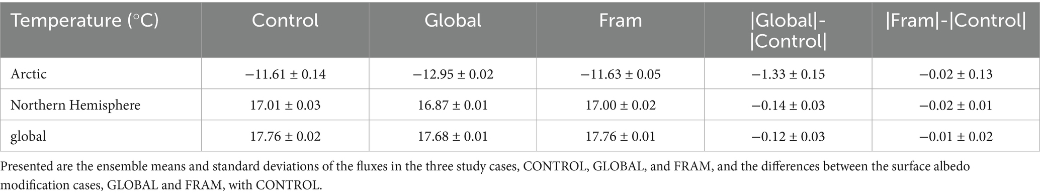
Table 2. Annual mean surface temperatures and temperature changes averaged across the Arctic (North of 70°N), Northern Hemisphere, and globally.

3.3 Changes in the atmospheric dynamics

The dominant Arctic atmospheric patterns (Sereze and Barry, 2005) in the winter consist of a high-pressure ridge stretching over the Beaufort Sea and East Siberian Shelf and strong easterly winds flowing from Eurasia toward the Canadian Archipelago, turning southward around Greenland (Supplementary Figure S3). These atmospheric dynamics transition in the late summer (JAS) to a basin-wide cyclonic system with a low surface pressure center near the Canadian Archipelago and counter-clockwise divergent winds (Supplementary Figure S3). Figure 4 shows the changes in the seasonal atmospheric dynamics due to the albedo perturbations in two sensitivity experiments, FRAM and GLOBAL.

During summer, when the albedo perturbation has its strongest impact, in the FRAM case, there is a dipole pattern of pressure anomalies with a strong positive anomaly center in the northern BS and two negative anomaly centers, respectively, in the Canadian Archipelago and the Nordic Seas, accompanied by intensified winds from the BS toward the Central Arctic and Beaufort Sea (Figure 4a). This pattern resembles the negative phase of the second dominant mode of variability in the Arctic, which has been found to be the main driver of the FS export (Tsukernik et al., 2009; Wu et al., 2006; Smedsrud et al., 2017). It is also similar to the anomalous dipole pattern linked to the extreme reduction in ice volume export observed in 2018 (Sumata et al., 2022). During the winter, this pressure anomaly expands and intensifies into a high-pressure ridge over the Eastern Arctic with intensified winds directed from BS and KS toward the Bering Strait (Figure 4b).

Figure 4

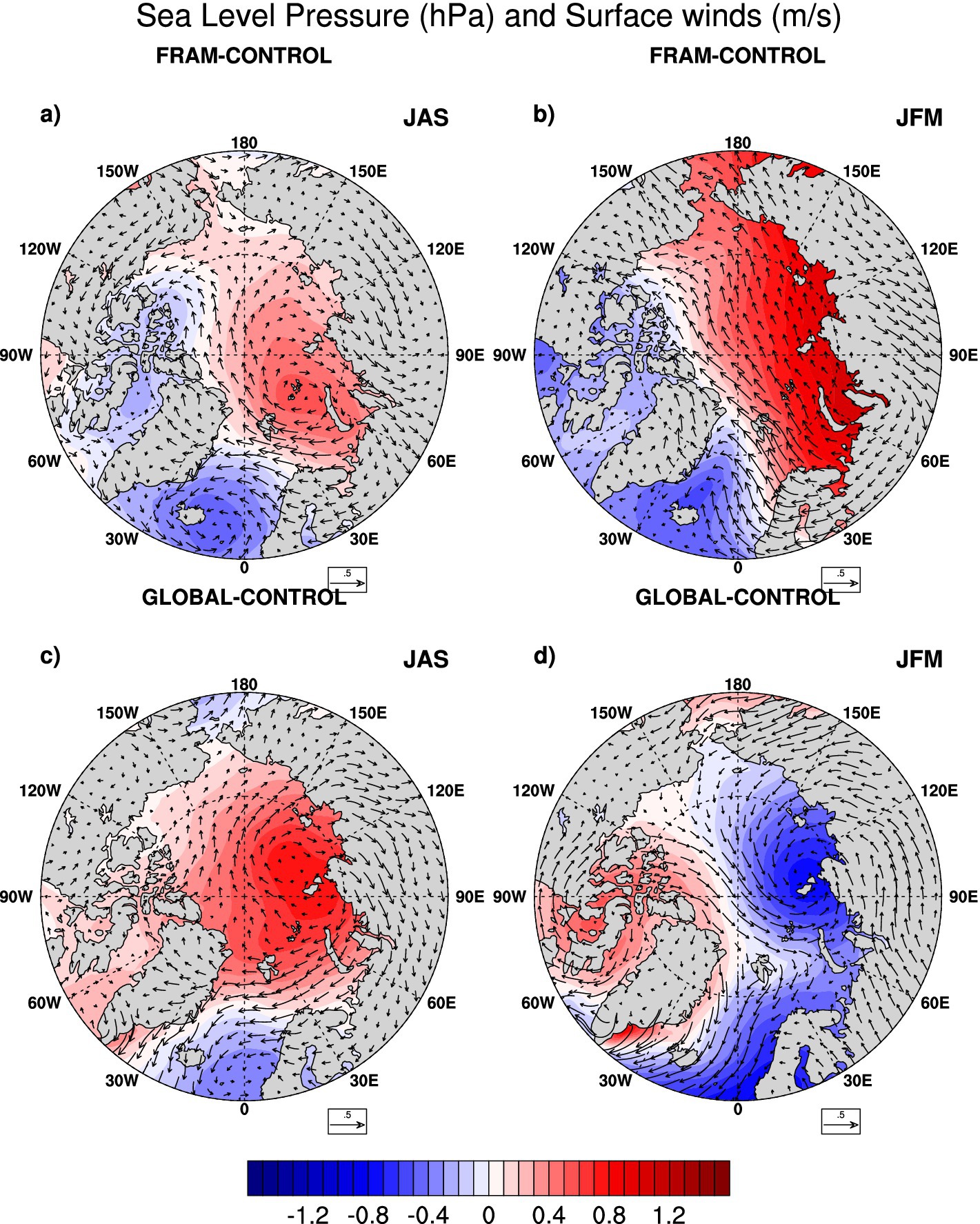
Figure 4. Changes of the seasonal sea level pressure (hPa) and surface winds (m/s) derived as ensemble mean differences averaged over the integration period 2001–2080 in two surface albedo modification cases (GLOBAL and FRAM) referred to the CONTROL case: (a) July–August–September (JAS) FRAM−CONTROL; (b) January–February–March (JFM) FRAM-CONTROL; (c) JAS GLOBAL−CONTROL; (d) JFM GLOBAL−CONTROL.

In contrast, in the GLOBAL case during winter (Figure 4d), there is a dipole of low sea level pressure anomaly in the Laptev Sea and high anomaly in the Canadian archipelago. In the summer, a basin-wide positive pressure anomaly centered in the Laptev Sea for the GLOBAL case (Figure 4c). In both seasons, the anomalous winds are favoring increased ice export through the FS.

3.4 Changes in sea ice

The largest changes in the sea ice concentration due to SAM applications are seen in the summer, particularly in the marginal zone in the GLOBAL case (Figure 5c), where the albedo perturbation is strongest (Figure 2a). During the winter season (Figures 5a,b), there are no significant ice concentration changes except near the ice edge in the North Atlantic. In the FRAM case, during the summer, there is a distinct increase in the sea ice concentration (12–14%) in the FS region of the albedo perturbation (Figure 5d). In both seasons, negative sea ice concentration anomalies in the Nordic Seas exist, possibly due to reduced Fram Strait ice export in the FRAM case (Figures 5b,d).

Figure 5

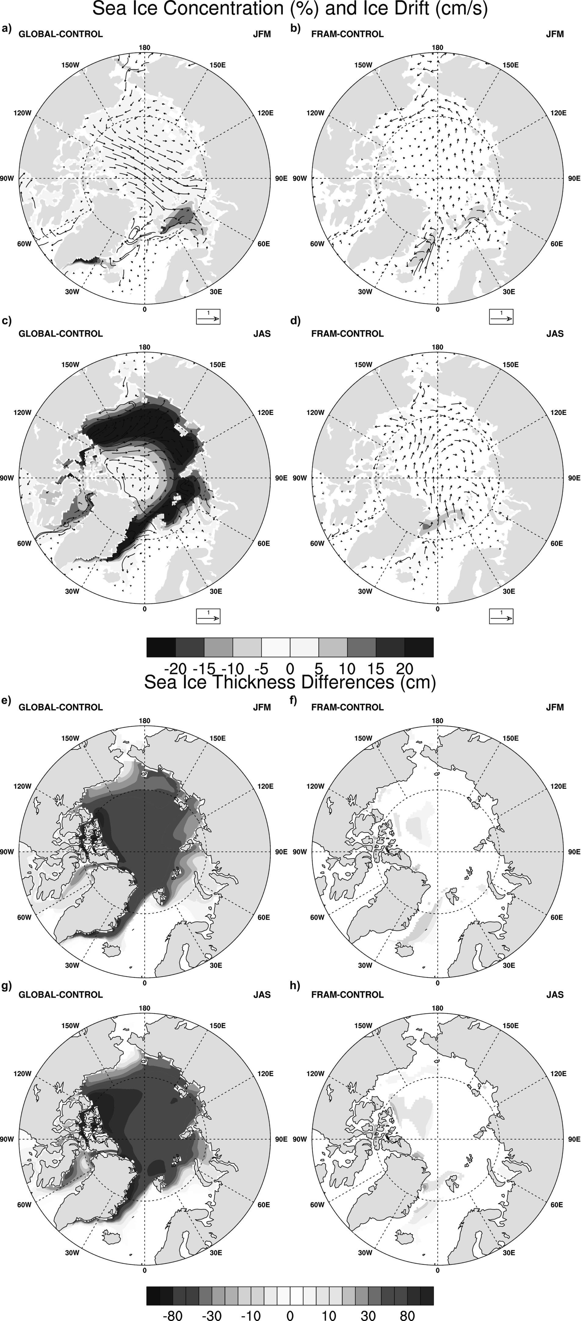
Figure 5. Arctic seasonal sea ice changes derived as ensemble mean differences averaged over the integration period 2001–2080 in two surface albedo modification cases (GLOBAL and FRAM) referred to CONTROL case: (a) GLOBAL-CONTROL sea ice concentration (%) and ice drift velocities (cm/s) changes in winter (January–February–March, JFM); (b) FRAM−CONTROL sea ice concentration (%) and ice drift velocities (cm/s) changes in winter (JFM); (c) GLOBAL−CONTROL sea ice concentration (%) and ice drift velocities (cm/s) changes in summer (July–August–September, JAS); (d) FRAM-CONTROL sea ice concentration (%) and ice drift velocities (cm/s) changes in summer (JAS); (e) GLOBAL−CONTROL sea ice thickness (CM) changes in winter (JFM); (f) FRAM−CONTROL sea ice thickness (cm) changes in winter (JFM); (g) GLOBAL−CONTROL sea ice thickness (cm) changes in summer (JAS); and (h) FRAM−CONTROL sea ice thickness (cm) changes in summer (JAS). The significance of the differences is evaluated using a two-tailed t-test. Only the statistically significant differences at a 90% confidence level are shown in color; the insignificant values are masked out.

Compared to changes in sea ice concentration, which primarily occur during the summer season when the SAM application has the greatest impact, changes in sea ice thickness persist throughout the year (Figures 5e–h). In the GLOBAL case, the ice thickens by approximately 1 m during the summer season in the Beaufort Sea and north of the Canadian Archipelago, and by approximately 80 cm across most of the rest of the basin (Figure 5g). These positive anomalies persist in the winter sea ice thickness distribution, although they are somewhat reduced (Figure 5e). In the FRAM case, significant thickening is found in the Central Arctic and north of the Canadian Archipelago, areas where the multi-year ice pack resides (Figure 5h). These thicker ice anomalies persist in the winter (Figure 5f), suggesting that they survived the summer melt season and may turn into multi-year ice. These non-local ice pack changes are related to the changes in the sea ice circulation (Figure 5d). An intensified drift moves the ice from the North Atlantic sector toward the Central Arctic during the summer. In the winter, the Transpolar Drift and the Beaufort Gyre are weakened, contributing to reduced sea ice export through the FS, therefore reducing ice concentration and thickness in the Nordic Seas. The major impact of the sea ice albedo enhancement is thickening of the sea ice pack, potentially increasing its multi-year fraction and longevity.

The simulated mean annual ice export in the CONTROL case is 627,581 km², which underestimates the observed long-term annual mean (Smedsrud et al., 2017) of 883,000 km² (Figure 6). Local thickening of the sea ice in the FS, as well as the changes in the Arctic ice circulation, are causing a reduction of the annual mean ice export by 14,979 km² (−2.4%) in the FRAM case, while in the case of Arctic-wide thickening of the Arctic ice pack (GLOBAL), the Fram export has increased by 235,491 km² (37.5%).

Figure 6

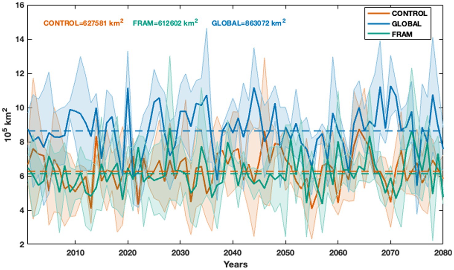
Figure 6. Annual time series of Fram Strait sea ice area export (km²) in CONTROL, GLOBAL, and FRAM. Solid lines are the ensemble mean annual time series, dashed lines are the climatological means, and the shadings represent the ensemble spreads.

3.5 Gain and efficacy

We evaluate the gain/loss of Arctic sea ice volume as the differences between GLOBAL/FRAM and CONTROL. Figure 7a shows the sea ice volume gain in % for the Northern Hemisphere, Arctic Ocean basin-wide, as well as in a variety of Arctic regions, North Atlantic and North Pacific marginal seas. In the GLOBAL case, there is ice volume gain in all regions, ranging from 10% in Hudson Bay to ~55% in the Canadian Archipelago. Overall, for the Arctic Ocean, the ice volume gain is ~42%. A significant increase in ice volume is observed in the Greenland Sea, suggesting enhanced sea ice export through the Fram Strait. This can be seen as a downside effect of the large-scale GLOBAL albedo treatment case since an excessive increase in the ice export will cause freshwater anomalies in the North Atlantic sector, consequently affecting the Atlantic thermohaline circulation. In the FRAM case, the ice volume gains are observed in the interior of the Arctic, specifically in the Central Arctic (0.4%), the Beaufort Sea (4.7%), and the Siberian sector (1.65%), resulting in an overall increase of 1.44% Arctic Ocean ice volume. There is ice volume loss in the North Atlantic sector, most significant in the Greenland Sea (−3.1%) and the Canadian Archipelago (−2.85%). These changes indicate reduced sea ice export in the Fram Strait and are a consequence of the changes in the sea ice drift seen previously (see Figures 5c,d), which tend to keep the sea ice in the interior of the Arctic Ocean.

Figure 7

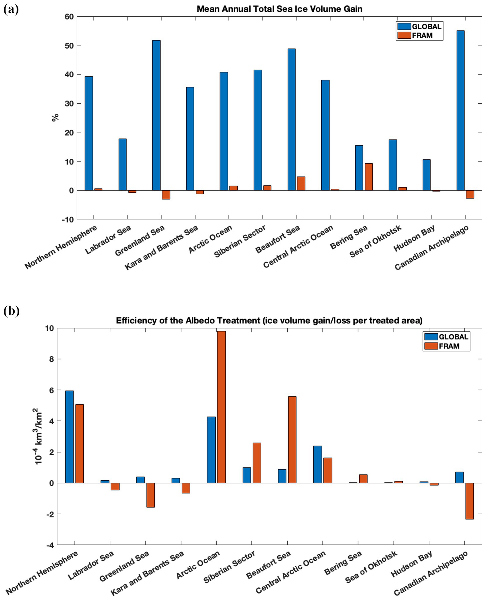
Figure 7. (a) Ice volume gain/loss (%) in a variety of Arctic regions; (b) Efficacy of the albedo treatment defined as ice volume gain/loss per 1 km² of treatment area in a variety of Arctic regions. The GLOBAL case is in blue; the FRAM case is in red.

We define the efficacy of the albedo treatment as the amount of ice volume gain per treatment area. Figure 7b compares the efficacies of the Arctic-wide albedo treatment (GLOBAL) and the regional albedo treatment in the Fram Strait (FRAM). This comparison reveals that the FRAM case is twice as efficient as the GLOBAL in restoring the sea ice volume of the Arctic Ocean. The most significant impacts are observed in the Beaufort Sea, the Siberian sector, and the Central Arctic Ocean, which is the central core of the Arctic ice pack. This implies that the FRAM case has the potential to recover the multi-year Arctic sea ice.

Our results show that increasing the treatment area does not proportionally increase the impact on the ice volume. In the FRAM case, each 1 km² of treated area increases the Arctic Ocean ice volume by 977,510 m³, whereas in the GLOBAL Arctic-wide albedo treatment, each 1 km² treated area increases the sea ice volume by half of that amount, 427,134 m³.

4 Discussion

4.1 Mechanisms

Our findings for the Fram Strait SAM application (Section 3) are synthesized in the schematic in Figure 8, which illustrates the mechanisms underlying the remote impacts on the Arctic sea ice cover and highlights the role of the thermodynamics−atmospheric dynamics interactions (Wu et al., 2006). The artificial SAM targeted in the Fram Strait enhances the surface albedo during the daylight season locally in the deployment region, but also in the vicinity outside the region, north of Svalbard, Barents Sea, and Kara Sea (Figure 8, block 1; Figure 3b). This non-local albedo enhancement can be attributed to the advection of thicker, higher-concentration ice from the FS region toward adjacent areas. The cooling temperature anomaly, due to the reduced absorption of solar radiation (Figure 8, block 2; Figures 1b,d,f), creates a high pressure anomaly in summer over KS and BS that extends into a high pressure ridge over eastern Arctic in winter and triggers a negative phase of the Arctic dipole (Figure 8, block 3; Figures 4b,d). This drives winds from the BS toward the Bering Sea along the Arctic dipole axis that modify the wind-driven large-scale sea ice circulation, weakening the Transpolar Drift and reducing the sea ice area export (Figure 8, block 4; Figures 5b,d, 6).

Figure 8

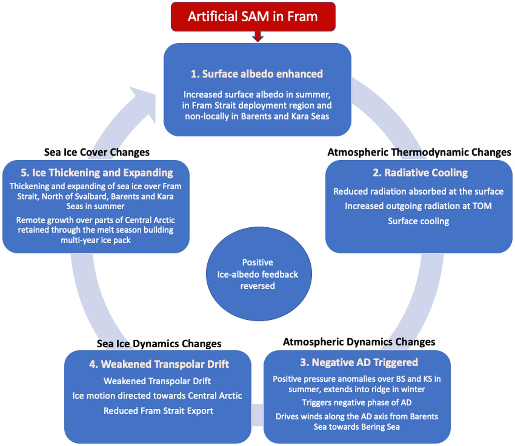
Figure 8. Schematic of the mechanisms of Arctic sea ice cover increase in the case of the Fram Strait region SAM application.

These large-scale atmospheric dynamics changes caused by the perturbed local radiation balance in the Fram Strait modify the large-scale ice circulation and generate dynamically driven non-local growth of the sea ice cover in the Central Arctic, within the Beaufort Gyre and north of the Canadian Archipelago (Figure 8, block 5; Figures 5f,h). Locally, in the Fram Strait region, the sea ice thickens and expands thermodynamically due to the direct impact of the SAM application. Although the albedo perturbation directly impacts sea ice cover during the summer, its indirect impacts persist in the winter, particularly in the Central Arctic. These results demonstrate the potential of the albedo treatment in the Fram Strait to restore the multi-year ice of the Arctic cover and reduce its loss via the Fram Strait. Once ice cover thickens and expands, its surface albedo increases naturally, reversing the ice–albedo feedback and promoting further ice growth and cooling.

4.2 Large-scale versus regional SAM applications

Large-scale, Arctic-wide SAM deployment could maximize benefits rapidly but is difficult to implement and carries higher risks of unintended side effects. Targeted small-scale interventions in key regions, such as the Fram Strait, are more feasible, cost-efficient, and likely to minimize adverse consequences while still supporting sea ice recovery.

The large-scale Arctic-wide SAM application (GLOBAL) in our study increases the ice volume basin-wide by almost 42% and the Fram Strait ice area export by 37% instantaneously. The latter creates a risk of excessive ice melt in the Nordic Seas, freshening and strengthening the ocean stratification and consequently slowing down the Atlantic Meridional Overturning Circulation (Ionita et al., 2016). The regional SAM application in the Fram Strait (FRAM) has a moderate effect on the total Arctic ice volume (1.44% gain); however, it increases ice volume by 4.7% in the remote Beaufort Sea and reduces the Fram Strait ice area export by 2.4%. A comparison of the efficacy of the two cases shows that the FRAM case is twice as efficient in restoring the Arctic Ocean sea ice volume per treatment area. These diverse impacts can be explained by differences in atmospheric dynamics and circulation changes between the two cases. In the FRAM case, atmospheric dynamics cause the sea ice to drift toward the central Arctic and reduce the Fram Strait ice export, thus retaining the sea ice within the Arctic basin. In the GLOBAL case, dynamics drive strong Transpolar Drift and increased Fram Strait ice export.

While the aim of the FRAM SAM application is to regulate ice loss through the FS and help maintain the Arctic ice mass balance, the largest ice loss is found in the marginal seas of the Arctic basin due to retreating ice edge (Onarheim et al., 2018) and snowline (Marcianesi et al., 2021), rapid thinning (Mallett et al., 2021) and high sensitivity to ice–albedo feedback (Rantanen et al., 2022). A possible strategy to achieve large-scale Arctic ice recovery would be the deployment of SAM across multiple strategic regions in tandem. Promising candidates include the Barents and Kara Seas—hotspots of Arctic amplification (Isaksen et al., 2022)—and the Beaufort Gyre, whose circulation could propagate the impacts of SAM perturbations across the basin. These areas also coincide with key centers of large-scale atmospheric circulation: the Beaufort High, a dominant high-pressure system over the western Arctic, and a semi-permanent low-pressure system over the Barents–Kara sector in the eastern Arctic (Serreze and Barrett, 2011). Targeted modification of the radiation balance in these regions, therefore, has the potential to trigger basin-wide shifts in atmospheric dynamics, thus dynamically redistributing and increasing the ice cover elsewhere, as demonstrated in our study.

4.3 Practical applications

Several engineering approaches have been proposed for implementing artificial surface albedo modification (SAM) in the Arctic using highly reflective materials (Ocean Visions, 2025). Some are applied at the ice surface, such as spreading layers of hollow glass microspheres (HGMs) (Field et al., 2018) and covering with geotextiles (Senese et al., 2020; Huss et al., 2021). Others are deployed in open water areas to increase the albedo at the ocean surface; for example, artificial sea foam or surface films to enhance reflectivity (Seitz, 2011; Aziz et al., 2014) and installation of reflective glass tiles (Haley and Nicklas, 2021).

The SAM simulation in our study most closely approximates the effects of the HGM layer. Applied on the ice surface, these microparticles act as a passive tracer that spreads with the drifting ice throughout the basin. A variety of commercially available HGMs have been tested in laboratory and small-pond field experiments to identify the most appropriate types for ice preservation applications. Initial laboratory tests (Field et al., 2018) and small-pond field tests (Johnson et al., 2022) showed an increase of surface albedo by 20%, which is close to the surface albedo modification magnitude used in our simulations. Latest laboratory measurements of a new variety of HGM, reported by Strawa et al. (2024), showed that the albedo increase of a 0.5-mm layer of HGM was 48.7%. These results set our current simulation on a conservative side, suggesting that new simulations with a higher SAM magnitude should be pursued.

While the above set of solutions is most effective during the sunlit months, an alternative approach, most efficient in wintertime, is to artificially thicken sea ice (thicker ice has higher albedo) by flooding the surface with seawater, which then refreezes to form an additional layer of ice (Desch et al., 2017). This method is limited to winter, when ocean temperatures beneath the ice exceed the air temperature above. Thickening the ice during the winter up to a meter improves its survival into summer by sustaining an albedo as high as 0.8 when combined with snow cover.

A possible long-term strategy for Arctic SAM could therefore combine these complementary methods—ice-surface or open-water albedo enhancement during summer and ice-thickening interventions during winter—to provide a coordinated, year-round treatment aimed at stabilizing and restoring Arctic sea ice. Note that all of these climate intervention solutions need to be properly vetted through ecological and environmental testing and active involvement of the affected communities, before practical implementation to ensure that they are safe, socially responsible, and environmentally sustainable (American Geophysical Union, 2025).

4.4 Limitations

This study has several limitations. First, longer integrations (>80 years) are necessary to fully spin up the deep ocean and capture Earth system variability on multi-decadal to centennial timescales, as highlighted by long-run model intercomparison studies (Rugenstein et al., 2019; Danabasoglu et al., 2020). Second, while the use of a constant greenhouse gas forcing, as in this study, provides a clean framework for isolating the albedo perturbation signal, it does not capture the transient variability associated with realistic emission pathways. Such idealized forcing experiments can bias estimates of the magnitude or persistence of climate feedbacks, since feedback strength is known to evolve with warming state and forcing pathway (Armour, 2017; Rugenstein et al., 2020). Future studies should therefore test the robustness of these responses under transient forcing scenarios. Third, the significance of the results would greatly improve if a larger number of ensemble members (>3) were used to better resolve the signal of the regional albedo perturbation in the Fram Strait, which is small compared to the Arctic-wide albedo perturbation. While the small ensemble size reflects computational constraints, the use of large ensembles has proven effective for improving signal-to-noise separation and quantifying internal variability in regional climate studies (Deser et al., 2012; Kay et al., 2015).

5 Conclusion

This study evaluated the potential of surface albedo modification (SAM) as an Arctic climate intervention, using climate model simulations of two scenarios: an Arctic-wide deployment (GLOBAL) and a localized application in the Fram Strait (FRAM).

In the GLOBAL case, SAM substantially enhances Arctic sea ice cover and cooling power. Net surface radiation decreases by 11.16 W/m² during the summer, while outgoing radiation at the top of the atmosphere increases by 10.70 W/m², thereby reducing radiative forcing. Annually, these changes amount to −3.57 W/m² at the surface and +2.14 W/m² at the TOA, corresponding to a 0.07 W/m² reduction globally and recovering approximately 10% of the present-day total Arctic sea ice radiative cooling effect. The basin-wide annual mean cooling by −1.33 °C is a magnitude over an order larger than the observed Arctic warming rate of 0.79 °C per decade (≈0.079 °C yr.⁻¹). At this rate, the anomaly corresponds to approximately 17 years of recent Arctic warming; however, this should be interpreted as an equilibrium offset rather than a delay in the warming trend, due to the equilibrated nature of the numerical experiment. The hemispheric and global mean cooling (−0.14 °C and −0.12 °C, respectively) are of the same order of magnitude as current warming trends. These results suggest that large-scale SAM could offset Arctic warming and contribute measurably to global cooling.

In addition, the Arctic-wide SAM increases basin-wide sea ice volume by 42% and enhances Fram Strait ice export by 37%. However, an excessive ice export carries risks of anomalous ice melt in the Nordic Seas, freshening and strengthening the ocean stratification, and potentially slowing down the Atlantic Meridional Overturning Circulation.

The regional targeted deployment in the Fram Strait (FRAM case) yields more spatially limited but dynamically significant responses. SAM applied in the Fram Strait enhances surface albedo both locally and in adjacent regions (Barents, Kara, and Central Arctic) through advection of thicker, more reflective ice. The resulting cooling anomaly alters atmospheric circulation, strengthening low-pressure systems over the Barents–Kara sector and triggering a negative Arctic dipole pattern. This reduces sea ice export through the Fram Strait via weakening the Transpolar Drift in addition to the local thickening and slowing of the ice in the FS region, supporting ice retention within the Arctic basin. This helps stabilize regions highly sensitive to albedo feedback and methane-clathrate release risk, such as the Barents and Kara Seas (Stolaroff et al., 2012).

In terms of the efficacy of the SAM application, our findings revealed that expanding the treatment area does not scale proportionally with the ice volume response. In the FRAM case, each square kilometer of treated area increases Arctic Ocean ice volume by ~977,510 m³, whereas in the GLOBAL Arctic-wide albedo treatment, 1 km² treated area increases the sea ice volume by half of that amount −427,134 m³.

While basin-wide SAM maximizes benefits, it is logistically challenging and carries a greater risk of unintended consequences. Targeted regional interventions, such as in Fram Strait, offer a more feasible and cost-effective alternative, with reduced risks and potential to stimulate basin-wide responses through atmosphere–ice–ocean interactions. Given that the largest ice losses occur in marginal seas—such as the Barents, Kara, and Beaufort—strategic SAM deployments in these regions may enhance Arctic-wide impacts. These areas are also dynamically linked to key atmospheric circulation centers (Beaufort High and Barents–Kara low), making them promising leverage points for intervention.

Overall, SAM emerges as a promising but complex strategy for Arctic climate intervention. A coordinated, regionally targeted, and seasonally adaptive deployment—combining albedo enhancement in summer with ice-thickening in winter—may offer the greatest potential for stabilizing Arctic sea ice while minimizing risks.

Data availability statement

The datasets presented in this study can be found in online repositories. The names of the repository/repositories and accession number(s) can be found at: DOI: 10.5281/zenodo.14782855.

Author contributions

DI: Conceptualization, Data curation, Formal analysis, Funding acquisition, Investigation, Methodology, Project administration, Resources, Software, Supervision, Validation, Visualization, Writing – original draft, Writing – review & editing. SB: Conceptualization, Formal analysis, Funding acquisition, Investigation, Methodology, Project administration, Supervision, Validation, Writing – original draft, Writing – review & editing. VM: Data curation, Formal analysis, Investigation, Methodology, Software, Writing – review & editing. AnS: Conceptualization, Funding acquisition, Project administration, Resources, Supervision, Writing – review & editing. LF: Conceptualization, Funding acquisition, Project administration, Resources, Supervision, Writing – review & editing. TP: Data curation, Software, Writing – review & editing. AlS: Data curation, Software, Writing – review & editing.

Funding

The author(s) declare that financial support was received for the research and/or publication of this article. The Arctic Ice Project (formerly Ice911 Research) provided funding and leadership for this work under contracts #051217 and #091618. Climformatics, Inc. volunteered time and effort in analyzing results and writing the article.

Acknowledgments

We thank Lars-Henrik Smesdrud for his comments on the manuscript and Alex Ivanov for preparing and uploading the input data on a public server. We acknowledge the use of IBM zCloud in running the spin-up simulations. We acknowledge the use of Sabalcore high-performance machines for all the ensemble simulations and analytics.

Conflict of interest

DI, SB, and VM were employed by Climformatics Inc.

The remaining authors declare that the research was conducted in the absence of any commercial or financial relationships that could be construed as a potential conflict of interest.

Generative AI statement

The authors declare that no Gen AI was used in the creation of this manuscript.

Any alternative text (alt text) provided alongside figures in this article has been generated by Frontiers with the support of artificial intelligence and reasonable efforts have been made to ensure accuracy, including review by the authors wherever possible. If you identify any issues, please contact us.

Publisher’s note

All claims expressed in this article are solely those of the authors and do not necessarily represent those of their affiliated organizations, or those of the publisher, the editors and the reviewers. Any product that may be evaluated in this article, or claim that may be made by its manufacturer, is not guaranteed or endorsed by the publisher.

Supplementary material

The Supplementary material for this article can be found online at: https://www.frontiersin.org/articles/10.3389/fclim.2025.1569470/full#supplementary-material

References

American Geophysical Union. (2025). Ethical Framework Report. Available online at: https://www.agu.org/ethicalframeworkprinciples.

Google Scholar

Armour, K. C. (2017). Energy budget constraints on climate sensitivity in light of inconstant climate feedbacks. Nat. Clim. Chang. 7, 331–335. doi: 10.1038/nclimate3278

Crossref Full Text | Google Scholar

Aziz, A., Hailes, H. C., Ward, J. M., and Evans, J. R. G. (2014). Long-term stabilization of reflective foams in sea water. RSC Adv. 4, 53028–53036. doi: 10.1039/C4RA08714C

Crossref Full Text | Google Scholar

Briegleb, B. P., and Light, B. (2007). A Delta-Eddington multiple scattering parameterization for solar radiation in the sea ice component of the community climate system model (No. NCAR/TN-472+STR). University Corporation for Atmospheric Research.

Google Scholar

Cvijanovic, I., Santer, B. D., Bonfils, C., Lucas, D. D., Chiang, J. C. H., and Zimmerman, S. (2017). Future loss of Arctic Sea-ice cover could drive a substantial decrease in California’s rainfall. Nat. Commun. 8:1947. doi: 10.1038/s41467-017-01907-4

PubMed Abstract | Crossref Full Text | Google Scholar

Dai, H. (2021). Roles of surface albedo, surface temperature and carbon dioxide in the seasonal variation of arctic amplification. Geophys. Res. Lett. 48:e2020GL090301. doi: 10.1029/2020GL090301

Crossref Full Text | Google Scholar

Danabasoglu, G., Lamarque, J.‐. F., Bacmeister, J., Bailey, D. A., DuVivier, A. K., Edwards, J., et al. (2020). The community earth system model version 2 (CESM2). J. Adv. Model. Earth Syst. 12:1916. doi: 10.1029/2019MS001916

Crossref Full Text | Google Scholar

Deser, C., Knutti, R., Solomon, S., and Phillips, A. S. (2012). Communication of the role of natural variability in future north American climate. Nat. Clim. Chang. 2, 775–779. doi: 10.1038/nclimate1562

Crossref Full Text | Google Scholar

Desch, S. J., Smith, N., Groppi, C., Vargas, P., Jackson, R., Kalyaan,, et al. (2017). Arctic ice management. Earth’s Future 5, 107–127. doi: 10.1002/2016EF000410

Crossref Full Text | Google Scholar

Duspayev, A., Flanner, M. G., and Riihelä, A. (2024). Earth’s sea ice radiative effect from 1980 to 2023. Geophys. Res. Lett. 51:e2024GL109608. doi: 10.1029/2024GL109608

Crossref Full Text | Google Scholar

Field, L., Ivanova, D., Bhattacharyya, S., Mlaker, V., Sholtz, A., Decca, R., et al. (2018). Increasing Arctic Sea ice albedo using localized reversible geoengineering. Earths Future 1:820. doi: 10.1002/2018EF000820

Crossref Full Text | Google Scholar

Haine, T. W., Curry, B., Gerdes, R., Hansen, E., Karcher, M., Lee, C., et al. (2015). Arctic freshwater export: status, mechanisms, and prospects. Glob. Planet. Change 125, 13–35. doi: 10.1016/j.gloplacha.2014.11.013

Crossref Full Text | Google Scholar

Haley, J. T., and Nicklas, J. M. (2021). Damping storms, reducing warming, and capturing carbon with floating, alkalizing, reflective glass tiles. London J. Res. Sci. 21, 11–20.

Google Scholar

Halvorsen, M. H., Smedsrud, L. H., Zhang, R., and Kloster, K. (2015). Fram Strait spring ice export and September Arctic Sea ice. Cryosphere Discuss. 9, 4205–4235. doi: 10.5194/tcd-9-4205-2015

Crossref Full Text | Google Scholar

Huss, M., Schwyn, U., Bauder, A., and Farinotti, D. (2021). Quantifying the overall effect of artificial glacier melt reduction in Switzerland, 2005–2019. Cold Reg. Sci. Technol. 184:103237. doi: 10.1016/j.coldregions.2021.103237

PubMed Abstract | Crossref Full Text | Google Scholar

Ionita, M., Scholz, P., Lohmann, G., Dima, M., and Prange, M. (2016). Linkages between atmospheric blocking, sea ice export through Fram Strait and the Atlantic meridional overturning circulation. Sci. Rep. 6:32881 (2016). doi: 10.1038/srep32881

PubMed Abstract | Crossref Full Text | Google Scholar

Isaksen, K., Nordli, Ø., Ivanov, B., Køltzow, M. A. Ø., Aaboe, S., Gjelten, H. M., et al. (2022). Exceptional warming over the Barents area. Sci. Rep. 12:9371. doi: 10.1038/s41598-022-13568-5

PubMed Abstract | Crossref Full Text | Google Scholar

Ivanova, D. (2025). Fram Strait: possible key to saving Arctic ice (version 1) [data set]. Zenodo.

Google Scholar

Johnson, D., Manzara, A., Field, L. A., Chamberlin, D. R., and Sholtz, A. (2022). A controlled experiment of surface albedo modification to reduce ice melt. Earths Future 10:e2022EF002883. doi: 10.1029/2022EF002883

Crossref Full Text | Google Scholar

Kay, J. E., Deser, C., Phillips, A., Mai, A., Hannay, C., Strand, G., et al. (2015). The community earth system model (CESM) large ensemble project. Bull. Am. Meteorol. Soc. 96, 1333–1349. doi: 10.1175/BAMS-D-13-00255.1

Crossref Full Text | Google Scholar

Landrum, L., and Holland, M. M. (2020). Extremes become routine in an emerging new Arctic. Nat. Clim. Chang. 10, 1108–1115. doi: 10.1038/s41558-020-0892-z

Crossref Full Text | Google Scholar

Lang, A., Yang, S., and Kaas, E. (2016). Sea ice thickness and recent Arctic warming. Geophys. Res. Lett. 44, 409–418. doi: 10.1002/2016GL071274

Crossref Full Text | Google Scholar

Mallett, R. D. C., Stroeve, J. C., Tsamados, M., Landy, J. C., Willatt, R., Nandan, V., et al. (2021). Faster decline and higher variability in the sea ice thickness of the marginal Arctic seas when accounting for dynamic snow cover. Cryosphere 15, 2429–2450. doi: 10.5194/tc-15-2429-2021

Crossref Full Text | Google Scholar

Marcianesi, F., Aulicino, G., and Wadhams, P. (2021). Arctic Sea ice and snow cover albedo variability and trends during the last three decades. Polar Sci. 28, 1873–9652. doi: 10.1016/j.polar.2020.100617

Crossref Full Text | Google Scholar

Ocean Visions. (2025) Arctic Sea Ice Road Map: Potential approaches to slow the loss of Arctic sea ice. Available online at: https://www2.oceanvisions.org/roadmaps/repair/arctic-sea-ice/ (Accessed August 25, 2025)

Google Scholar

Onarheim, I. H., Eldevik, T., Smedsrud, L. H., and Stroeve, J. C. (2018). Seasonal and regional manifestation of Arctic Sea ice loss. J. Clim. 31, 4917–4932. doi: 10.1175/JCLI-D-17-0427.1

Crossref Full Text | Google Scholar

Overland, J. E., and Wang, M. (2013). When will the summer Arctic be nearly sea ice free. Geophys. Res. Lett. 40, 2097–2101. doi: 10.1002/grl.50316

Crossref Full Text | Google Scholar

Pistone, K., Eisenman, I., and Ramanathan, V. (2014). Observational determination of albedo decrease caused by vanishing Arctic Sea ice. Proc. Natl. Acad. Sci. U. S. A. 111, 3322–3326. doi: 10.1073/pnas.1318201111

PubMed Abstract | Crossref Full Text | Google Scholar

Pistone, K., Eisenman, I., and Ramanathan, V. (2019). Radiative heating of an ice-free Arctic Ocean. Geophys. Res. Lett. 46, 7474–7480. doi: 10.1029/2019GL082914

Crossref Full Text | Google Scholar

Previdi, M., and Simmonds, I. (2021). Arctic amplification of climate change: a review of underlying mechanisms. Environ. Res. Lett. 16:093003. doi: 10.1088/1748-9326/ac1c29

Crossref Full Text | Google Scholar

Rantanen, M., Karpechko, A. Y., Lipponen, A., Nordling, K., Hyvärinen, O., Ruosteenoja, K., et al. (2022). The Arctic has warmed nearly four times faster than the globe since 1979. Commun. Earth Environ. 3:168. doi: 10.1038/s43247-022-00498-3

Crossref Full Text | Google Scholar

Richter-Menge, J., Druckenmiller, M., and Jeffries, M. (2019). Arctic report card. Available online at: https://www.arctic.noaa.gov/Report-Card.

Google Scholar

Rugenstein, M., Bloch-Johnson, J., Gregory, J., Andrews, T., Mauritsen, T., Li, C., et al. (2020). Equilibrium climate sensitivity estimated by equilibrating climate models. Geophys. Res. Lett. 47:898. doi: 10.1029/2019GL083898

Crossref Full Text | Google Scholar

Rugenstein, M. A. A., Rugenstein, M., Bloch-Johnson, J., Abe-Ouchi, A., Andrews, T., Beyerle, U., et al. (2019). Longrunmip: motivation and design for a large collection of millennial-length AOGCM simulations. Bull. Am. Meteorol. Soc. 100, 2551–2570. doi: 10.1175/BAMS-D-19-0068.1

Crossref Full Text | Google Scholar

Screen, J. A., Simmonds, I., and Keay, K. (2011). Dramatic interannual changes of perennial Arctic Sea ice linked to abnormal summer storm activity. J. Geophys. Res. 116:D15105. doi: 10.1029/2011JD015847

Crossref Full Text | Google Scholar

Seitz, R. (2011). Bright water: hydrosols, water conservation and climate change. Clim. Chang. 105, 365–381. doi: 10.1007/s10584-010-9965-8

Crossref Full Text | Google Scholar

Senese, A., Azzoni, R. S., Maragno, D., D’Agata, C., Fugazza, D., Mosconi, B., et al. (2020). The non-woven geotextiles as strategies for mitigating the impacts of climate change on glaciers. Cold Reg. Sci. Technol. 173:103007. doi: 10.1016/j.coldregions.2020.103007

Crossref Full Text | Google Scholar

Sereze, M. C., and Barry, R. G. (2005). The Arctic climate system. Cambridge, England: Cambridge University Press.

Google Scholar

Serreze, M. C., and Barrett, A. P. (2011). Characteristics of the Beaufort Sea high. J. Clim. 24, 159–182. doi: 10.1175/2010JCLI3636.1

Crossref Full Text | Google Scholar

Smedsrud, L. H., Halvorsen, M. H., Stroeve, J. C., Zhang, R., and Kloster, K. (2017). Fram strait sea ice export variability and September Arctic Sea ice extent over the last 80 years. Cryosphere 11, 65–79. doi: 10.5194/tc-11-65-2017

Crossref Full Text | Google Scholar

Smedsrud, L. H., Sirevaag, A., Kloster, K., Sorteberg, A., and Sandven, S. (2011). Recent wind driven high sea ice area export in the Fram Strait contributes to Arctic Sea ice decline. Cryosphere 5, 821–829. doi: 10.5194/tc-5-821-2011

Crossref Full Text | Google Scholar

Spall, M. (2019). Dynamics and thermodynamics of the mean transpolar drift and ice thickness in the Arctic Ocean. J. Clim. 32, 8449–8463. doi: 10.1175/JCLI-D-19-0252.1

Crossref Full Text | Google Scholar

Spreen, G., de Steur, L., Divine, D., Gerland, S., Hansen, E., and Kwok, R. (2020). Arctic sea ice volume export through Fram Strait from 1992 to 2014. J. Geophys. Res. Oceans. 125:e2019JC016039. doi: 10.1029/2019JC016039

Crossref Full Text | Google Scholar

Stolaroff, J. K., Bhattacharyya, S., Smith, C. A., Bourcier, W. L., Cameron-Smith, P. J., and Aines, R. A. (2012). Review of methane mitigation technologies with application to rapid release of methane from the Arctic. Environ. Sci. Technol. 46, 6455–6469. doi: 10.1021/es204686w

PubMed Abstract | Crossref Full Text | Google Scholar

Strawa, A., Olinger, S., Zornetzer, S., Johnson, D., Bhattacharyya, S., Ivanova, D., et al. (2024). Application of hollow glass microspheres in the Arctic Ocean would likely Lead to a deceleration of Arctic Sea ice loss - a critique of the paper by Webster and Warren (2022). Earths Future 13:4749. doi: 10.1029/2024EF004749

Crossref Full Text | Google Scholar

Sumata, H., de Steur, L., Gerland, S., Divine, D. V., and Pavlova, O. (2022). Unprecedented decline of Arctic Sea ice outflow in 2018. Nat. Commun. 13:1747. doi: 10.1038/s41467-022-29470-7

PubMed Abstract | Crossref Full Text | Google Scholar

Thackeray, C. W., and Hall, A. (2019). An emergent constraint on future Arctic Sea-ice albedo feedback. Nat. Clim. Chang. 9, 972–978. doi: 10.1038/s41558-019-0619-1

Crossref Full Text | Google Scholar

Thompson, D. W. J., and Wallace, J. M. (2000). Annular modes in the extratropical circulation. Part I: Month-to-Month Variability. J. Clim. 13, 1000–1016. doi: 10.1175/1520-0442(2000)013<1000:AMITEC>2.0.CO;2

Crossref Full Text | Google Scholar

Tsukernik, M., Deser, C., Alexander, M., and Tomas, R. (2009). Atmospheric forcing of Fram Strait sea ice export: a closer look. Clim. Dyn. 35, 1349–1360. doi: 10.1007/s00382-009-0647-z

Crossref Full Text | Google Scholar

Vihma, T. (2014). Effects of Arctic Sea ice decline on weather and climate: a review. Surv. Geophys. 35, 1175–1214. doi: 10.1007/s10712-014-9284-0

Crossref Full Text | Google Scholar

Vihma, T., Tisler, P., and Uotila, P. (2012). Atmospheric forcing on the drift of Arctic Sea ice in 1989–2009. Geophys. Res. Lett. 39:L02501. doi: 10.1029/2011GL050118

PubMed Abstract | Crossref Full Text | Google Scholar

Williams, J., Tremblay, B., Newton, R., and Allard, R. (2016). Dynamic preconditioning of the minimum September Sea-ice extent. J. Clim. 29, 5879–5891. doi: 10.1175/JCLI-D-15-0515.1

Crossref Full Text | Google Scholar

Wu, B., and Johnson, M. (2007). A seesaw structure in SLP anomalies between the Beaufort Sea and the Barents Sea. Geophys. Res. Lett. 34:L05811. doi: 10.1029/2006GL028333

Crossref Full Text | Google Scholar

Wu, B., Wang, J., and Walsh, J. E. (2006). Dipole anomaly in the winter Arctic atmosphere and its association with sea ice motion. J. Clim. 19, 210–225. doi: 10.1175/JCLI3619.1

Crossref Full Text | Google Scholar

Zhang, R., Wang, H., Fu, Q., Rasch, P. J., and Wang, X. (2019). Unraveling driving forces explaining significant reduction in satellite-inferred Arctic surface albedo since the 1980s. Proc. Natl. Acad. Sci. 116, 23947–23953. doi: 10.1073/pnas.1915258116

PubMed Abstract | Crossref Full Text | Google Scholar