An algebra for local histograms

1. Introduction

Inspired by Koenderink and Doorn (1999), we have for many years worked with images, and features derived from local histograms, and a nagging question has been, what the degrees of freedoms remain, given a set of overlapping histograms. This paper presents a theoretical investigation into the relationship between sets of local histograms and functions between discrete domains and codomains of any dimension. We describe an algebra of histograms, which is strongly related to the algebra of sets on the function domain and multisets: Given a set of local histogram's domains, h(X_i), X_i ⊂ X, where X is the full domain, and X_i are subsets thereof, such that ⋃_iX_i = X, we factor X into a new set of disjoint subsets $\left\{X_j^{\prime }\right\},{\bigcup }_j{X}_j^{\prime }=X$, and with this, we are able to count the number of independent histograms, which jointly describe the total set of local histograms, and which leads to a simple countable, generative model for functions drawn from these histograms. Finally, we present a simple algorithm for generating the set of functions, which share a particular set of local histograms overlapping or not.

Our work is an extension of Sporring and Darkner (2022), where 1-dimensional signals are considered and the concept of metameric classes is introduced in the concept of local histograms. The article restricts itself to binary signals from their densely overlapping histograms. In Wu et al. (2000), the authors consider normalized histogram of images filtered with Gabor kernels (Gabor, 1946), and in particular, the limiting case of the discrete domain converging to ℤ².

This paper is organized as follows. In Section 2, we present the histogram-algebra, in Section 3 we show how the number of unique functions sharing a specific set of histograms is generated. In Section 4, we present the algorithm for calculating the set of functions, which share a given set of local histograms, and finally, Section 6 gives concluding remarks.

2. Histograms as Infintely-Additive set functions

In the following, we will define an algebra for discrete histograms of disjoint domains, and we will extend this to non-disjoint domains by repartitioning domains.

Consider discrete domain X, co-domain A, and a functions f : X → A between them, such that the histogram h : A → ℤ₊

$\begin{array}{ll}{h}_X(a)={\displaystyle \sum _{x\in X}}\delta (f(x)-a),& (\mathrm{1a})\end{array}$

$\begin{array}{ll}\delta (x)=\{\begin{array}{l}1,\text{ when }x=0,\hfill \\ 0,\text{ otherwise},\hfill \end{array}& (\mathrm{1b})\end{array}$

is defined. Conceptually, we think of X as d-dimensional spatial domain X = {1, 2, 3, …, n}^d with side-lengths n > 0, and A as a an alphabet of m > 0 different gray values A = {1, …m}, but for the properties of possibly overlapping histograms, the interpretation of the values of X and A is not important, and X and A could as well be the set {cow, cat, fish} or color triplets {(0, 0, 0), (0, 0, 1), …}. As long as we can define a one-to-one mapping to an index set, we need only to concern ourselves with this index.

Two key properties of a histogram are that

Property 2.1. Histograms are non-negative, ∀_a∈Ah(a) ≥ 0.

Property 2.2. Every value f(x), x ∈ X is counted once and only once.

A direct consequence of Property 2.2 is that

$\begin{array}{ll}{\displaystyle \sum _{a\in A}}{h}_X(a)=\left|X\right|.& (2)\end{array}$

In this article, we are interested in counting possible histograms and for given histograms, counting the number of possible function. Let's start by examining the number of unique histograms that exists for a single domain and co-domain. Let ${{H}}_X=\left\{h_X^i\right\},{\forall }_{i,j}{h}_X^i\ne h_X^j$ be the set of unique histograms. Its size may be calculated as unordered sampling with replacement, where we visually represent each element in X with a “•” and each bin edge with a “;.” Then the string “• • •; •;;…” corresponds to the histogram [1; 2; 3; …] → [3; 1; 0; …]. For brevity, it is convenient to assume that an ordering of the alphabet exists such that we may write the before mentioned histogram simply as [3; 1; 0; …]. The string will be |X|+|A|−1 long, and all possible histograms can be produced by selecting |A| − 1 positions in this string for the “;” character. Thus, the number of unique histograms for a given domain X is given by the binomial coefficient,

$\begin{array}{ll}|{\mathscr{H}}_X|=\left(\begin{array}{c}\left|X\right|+\left|A\right|-1\\ \left|A\right|-1\end{array}\right)=\left(\begin{array}{c}\left|X\right|+\left|A\right|-1\\ \left|X\right|\end{array}\right).& (3)\end{array}$

In the following, we will consider possibly overlapping, local histograms over the domain X. Our expositions will be divided into first non-overlapping or disjoint domains, and then we will show how overlapping domains can be repartitioned into disjoint domains, and how these relate to the original overlapping domains.

2.1. Histograms over disjoint domains

Consider a partitioning of X into k < ∞ disjoint subdomains $X={\bigcup }_{i=1}^k{X}_i$, where ∀_i≠jX_i ∩ X_j = ∅. Due to Property 2.2, h is a finitely-additive set function (Stover, 2022), and hence,

$\begin{array}{ll}{\displaystyle \sum _{i=1}^k}{h}_{X_i}(a)=h_{{\displaystyle {\bigcup }_i}{X}_i}(a)=h_X(a).& (4)\end{array}$

As a consequence, h_∅(a) = 0, and addition of histograms of disjoint domains is commutative and associative. The subtraction h_Y(a) − h_X(a) is a histogram when X ⊆ Y, e.g.,

$\begin{array}{ll}{h}_{X\cup Y}=h_X+h_Y\iff h_{X\cup Y}-h_X=h_Y\iff h_{X\cup Y}-h_Y=h_X,& (5)\end{array}$

omitting the argument a for brevity. However, subtracting any two histograms in general will likely produce negative values violating Property 2.1, and although useful at times, the result will not be a histogram.

Since the sets X_i are disjoint, the size of the set of all possible histograms of X is found by extending Equation (3) directly,

$\begin{array}{ll}|\mathscr{H}|={\displaystyle \prod _{i=1}^k|{\mathscr{H}}_{X_i}|.}& (6)\end{array}$

2.2. Partitioning of non-disjoint sets

For a set of k non-disjoint domains ${X}=\left\{X_i\right\}$ of $X={\bigcup }_{i=1}^k{X}_i$, we can repartition X into disjoint domains of unique overlap of X_i

$\begin{array}{ll}{X}_I^{\prime }=\left({\displaystyle \bigcap _{j\in I}}{X}_j\right)\backslash \left({\displaystyle \bigcup _{j\in \left\{0,1,\dots n-1\right\}\backslash I}}{X}_j\right),I\in P_k,& (7)\end{array}$

where P_k is the powerset of {1, 2, …, k}, e.g., P₃ = {∅, {1}, {2}, {3}, {1, 2}, {1, 3}, {2, 3}, {1, 2, 3}}. With this notation, we find the original sets as,

$\begin{array}{ll}{X}_i={\displaystyle \bigcup _{p\in P_k:i\in p}}{X}_p^{\prime }.& (8)\end{array}$

Example 2.1. As an example, consider 3 sets X₁, X₂, and X₃, there are 7 unqiue intersections as illustrated in Figure 1 together with the powerset naming convention.

FIGURE 1

Figure 1. The naming convention for generating unique, non-overlapping domain parts are identified from X₀, X₁, and X₂.

That is, $X_{\left\{1,2\right\}}^{\prime }=(X_1\cap X_2)\backslash X_3$ and $X_1=X_{\left\{1\right\}}^{\prime }\cup X_{\left\{1,2\right\}}^{\prime }\cup X_{\left\{1,2,3\right\}}^{\prime }\cup X_{\left\{1,3\right\}}^{\prime }$.

Example 2.2. As a concrete example, consider the domain X = {1, 2, …, 6} and the codomain A = {1, 2, 3}, and define X₁ = {1, 2, 3, 4}, X₂ = {3, 4, 5, 6}. Assuming the usual ordering of integers, we can illustrate this overlap on a line as,

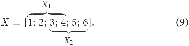
Using Equation (7) we find that P₂ = {{1}, {2}, {1, 2}} and that $X_{\left\{1\right\}}^{\prime }=\left\{1,2\right\}$, $X_{\left\{1,2\right\}}^{\prime }=\left\{3,4\right\}$, and $X_{\left\{2\right\}}^{\prime }=\left\{5,6\right\}$. Each of these subdomains are of size 2, and thus, the by Equation (3), number of possible histograms of each is $\left(\begin{array}{c}2+3-1\\ 3-1\end{array}\right)=6$, and the set of possible histograms is

$\begin{array}{l}{{H}}_{X_I}=\left\{\left[2;0;0\right],\left[1;1;0\right],\left[1;0;1\right],\left[0;2;0\right],\left[0;1;1\right],\left[0;0;2\right]\right\},\end{array}$

$\begin{array}{ll}I\in P_2.& (10)\end{array}$

Since there are 3 disjoint regions each with 6 possible histograms, there are 6³ = 216 combinations of these. Introducing a natural extension of our notations on the domains to their corresponding histograms, one of these is,

$\begin{array}{ll}{h}_{\left\{1\right\}}=h_{X_{\left\{1\right\}}^{\prime }}=\left[1;1;0\right],& (\mathrm{11a})\end{array}$

$\begin{array}{ll}{h}_{\left\{1,2\right\}}=h_{X_{\left\{1,2\right\}}^{\prime }}=\left[1;0;1\right],& (\mathrm{11b})\end{array}$

$\begin{array}{ll}{h}_{\left\{2\right\}}=h_{X_{\left\{2\right\}}^{\prime }}=\left[0;2;0\right],& (\mathrm{11c})\end{array}$

in which case,

$\begin{array}{ll}{h}_1=h_{X_1}=h_{\left\{1\right\}}+h_{\left\{1,2\right\}}=\left[1;1;0\right]+\left[1;0;1\right]=\left[2;1;1\right]& (\mathrm{12a})\end{array}$

$\begin{array}{ll}{h}_2=h_{X_2}=h_{\left\{1,2\right\}}+h_{\left\{2\right\}}=\left[1;0;1\right]+\left[0;2;0\right]=\left[1;2;1\right].& (\mathrm{12b})\end{array}$

Since these overlapping histograms have been generated by histograms on their disjoint parts, we are sure that a function exists on X which has histograms h₁ and h₂. Further, since histograms are finitely-additive functions we are sure that Properties 2.1 and 2.2 are fulfilled for h₁ and h₂.

In the following, we will count the number of functions on disjoint domains and see how these can be combined to generate the family of functions, which share overlapping histograms generated from the disjoint domains.

3. Unique functions and their histograms on disjoint domains

For a single domain X, the total number of possible functions is given as |A|^|X|, and some of these have the same histogram. Conversely, given a histogram h, the set of functions, which share this histogram can be produced as the set of distinct permutations of the function,

$\begin{array}{ll}S=[\stackrel{\left|X\right|}{\overbrace{\underset{h(1)}{\underbrace{1;\mathrm{\dots };1}};\underset{h(2)}{\underbrace{2;\mathrm{\dots };2}};\underset{h(3)}{\underbrace{3;\mathrm{\dots };3}};\mathrm{\dots }]}}.& (13)\end{array}$

The number of distinct functions is given by

$\begin{array}{ll}\begin{array}{l}{C}_X={\displaystyle \prod _{i=1}^{\left|A\right|}\left(\frac{\left|X\right|-c_X(i)}{h_X(i)}\right)},\hfill \end{array}& (\mathrm{14a})\end{array}$

$\begin{array}{ll}{c}_X(i)=\{\begin{array}{ll}0,\hfill & i\le 1\hfill \\ {\displaystyle {\sum }_{j=1}^i{h}_X(j),}\hfill & \text{ otherwise}.\hfill \end{array}& (\mathrm{14b})\end{array}$

C_X is a multinomial coefficient and can be simplified to

$\begin{array}{ll}{C}_X=\left(\begin{array}{c}\left|X\right|-c(1)\\ h(1)\end{array}\right)\left(\begin{array}{c}\left|X\right|-c(2)\\ h(2)\end{array}\right)\left(\begin{array}{c}\left|X\right|-c(3)\\ h(3)\end{array}\right)\dots ,& (\mathrm{15a})\end{array}$

$\begin{array}{ll}=\left(\begin{array}{c}\left|X\right|\\ h(1)\end{array}\right)\left(\begin{array}{c}\left|X\right|-h(1)\\ h(2)\end{array}\right)\left(\begin{array}{c}\left|X\right|-h(1)-h(2)\\ h(3)\end{array}\right)\dots ,& (\mathrm{15b})\end{array}$

$\begin{array}{l}=\frac{\left|X\right|!}{h(1)!(\left|X\right|-h(1))!}\frac{(\left|X\right|-h(1))!}{h(2)!(\left|X\right|-h(1)-h(2))!}\end{array}$

$\begin{array}{ll}\frac{(\left|X\right|-h(1)-h(2))!}{h(3)!(\left|X\right|-h(1)-h(2)-h(3))!}\dots ,& (\mathrm{15c})\end{array}$

$\begin{array}{ll}=\frac{\left|X\right|!}{h(1)!h(2)!h(3)!\dots },& (\mathrm{15d})\end{array}$

$\begin{array}{ll}=\frac{\left|X\right|!}{{\displaystyle {\prod }_{i=1}^{\left|A\right|}}h(i)!},& (15e)\end{array}$

where we for simplicity have neglected to write the subscript X and in the last term used that (|X|−h(1)−h(2)−…−h(|A|))! = 1. Like the simplified notation for h, we will also write C_i for C_Xi.

For the disjoint sets ∀_i≠jX_i ∩ X_j = ∅, the functions on X_i are independent on those on X_j, j ≠ i, and may be chosen independently. Thus, number of functions sharing H is

$\begin{array}{ll}{C}_X^{\text{disjoint}}={\displaystyle \prod _i}{C}_{X_i},& (16)\end{array}$

where C_Xi is Equation (14) applied to h_i.

Example 3.1. As an example, consider the (ordered) alphabet A = {1, 2, 3} and the histogram h_X = [1; 1; 2]. Then by Equation (2) we know that |X| = 4. Finally using Equation (15) we find that

$\begin{array}{ll}{C}_X=\frac{4!}{1!1!2!}=12.& (17)\end{array}$

Assuming that X is a line, we can list all possible functions which has histogram h_X as,

$\begin{array}{l}[0;1;2;2],[0;2;1;2],[0;2;2;1],[1;0;2;2],[2;0;1;2],[2;0;2;1],\hfill \\ [1;2;0;2],[2;1;0;2],[2;2;0;1],[1;2;2;0],[2;1;2;0],[2;2;1;0].\hfill \end{array}$

Example 3.2. Another example, for the same alphabet as in Example 3.1 but with h_X = [2; 0; 2] we follow the same procedure as in Example 3.1 to calculate $C=\frac{4!}{0!2!2!}=6$, and the list possible functions on a linear domain X as,

$\begin{array}{l}\left[0;0;2;2\right],\left[0;2;0;2\right],\left[0;2;2;0\right],\left[2;0;0;2\right],\left[2;0;2;0\right],\left[2;2;0;0\right].\end{array}$

Example 3.3. Continuing Example 2.2 with A = {1, 2, 3}, X = {1, 2, …, 6}, X₁ = {1, 2, 3, 4}, X₂ = {3, 4, 5, 6}, and h_{1} = [1; 1; 0], h_{1,2} = [1; 0; 1], h_{2} = [0; 2; 0], the number of functions is computed from its non-overlapping parts are

$\begin{array}{l}{C}_{\left\{1\right\}}=\frac{2!}{1!1!0!}=2,C_{\left\{1,2\right\}}=\frac{2!}{1!0!1!}=2,\end{array}$

$\begin{array}{ll}{C}_{\left\{2\right\}}=\frac{2!}{0!2!0!}=1,& (18)\end{array}$

Thus, the total number of functions for these specific histograms h₀ and h₁ is C_{1}C_{1,2}C_{2} = 4, and the functions are any combination of

$\begin{array}{l}f(X_{\left\{1\right\}}^{\prime })\in \left\{\left[1;2\right],\left[2;1\right]\right\},f(X_{\left\{1,2\right\}}^{\prime })\in \left\{\left[1;3\right],\left[3;1\right]\right\},\end{array}$

$\begin{array}{ll}f(X_{\left\{2\right\}}^{\prime })=\left[2;2\right].& (19)\end{array}$

One of the 4 functions, which have histograms h₁ and h₂ specified in Equation (12) is thus $f(X)=f(X_{\left\{1\right\}}^{\prime }\cup X_{\left\{1,2\right\}}^{\prime }\cup X_{\left\{2\right\}}^{\prime })=\left[1;2;3;1;2;2\right]$.

Example 3.4. As a final example, consider a one-dimensional function over the alphabet A = {1, 2, 3} and where X = X₁ ∪ X₂ ∪ X₃, X₁ = {1, 2, 3, 4}, X₂ = {2, 3, 4, 5}, X₃ = {3, 4, 5, 6}. The unique partitions are then given as,

$\begin{array}{l}{X}_{\left\{1\right\}}^{\prime }=\left\{1\right\},X_{\left\{1,2\right\}}^{\prime }=\left\{2\right\},X_{\left\{1,3\right\}}^{\prime }=\varnothing ,X_{\left\{1,2,3\right\}}^{\prime }=\left\{3,4\right\},\end{array}$

$\begin{array}{ll}{X}_{\left\{2\right\}}^{\prime }=\varnothing ,X_{\left\{2,3\right\}}^{\prime }=\left\{5\right\},X_{\left\{3\right\}}^{\prime }=\left\{6\right\}.& (20)\end{array}$

The possible histograms of the singleton domains are

$\begin{array}{ll}{h}_I\in \left\{\left[1;0;0\right],\left[0;1;0\right],\left[0;0;1\right]\right\},I\in \left\{\left\{1\right\},\left\{1,2\right\},\left\{2,3\right\},\left\{3\right\}\right\},& (21)\end{array}$

and for $X_{\left\{1,2,3\right\}}^{\prime }$,

$\begin{array}{ll}{h}_{\left\{1,2,3\right\}}\in \left\{\left[2;0;0\right],\left[1;1;0\right],\left[1;0;1\right],\left[0;2;0\right],\left[0;1;1\right],\left[0;0;2\right]\right\},& (22)\end{array}$

since $\left|X_{\left\{1,2,3\right\}}^{\prime }\right|=2$. The total number of different histograms is,

$\begin{array}{ll}|\mathscr{H}|={\left(\begin{array}{c}3\\ 2\end{array}\right)}^4\left(\begin{array}{c}4\\ 2\end{array}\right)=486.& (23)\end{array}$

To generate a set of functions and overlapping histograms, we choose a specific set of h_I,

$\begin{array}{l}{h}_{\left\{1\right\}}=\left[0;0;1\right],h_{\left\{1,2\right\}}=\left[0;1;0\right],h_{\left\{1,2,3\right\}}=\left[1;1;0\right],\end{array}$

$\begin{array}{ll}{h}_{\left\{2,3\right\}}=\left[0;0;1\right],h_{\left\{3\right\}}=\left[1;0;0\right],& (24)\end{array}$

and thus, h₁ = h_{1} + h_{1,2} + h_{1,2,3} = [1; 2; 1], h₂ = h_{1,2} +h_{1,2,3} +h_{2,3} = [1; 2; 1], and h₃ = h_{1,2,3} +h_{2,3} +h_{3} = [2; 1; 1]. The number of functions is computed from its non-overlapping parts,

$\begin{array}{ll}{C}_{\left\{1\right\}}=1,C_{\left\{1,2\right\}}=1,C_{\left\{1,2,3\right\}}=2,C_{\left\{2,3\right\}}=1,C_{\left\{3\right\}}=1,& (25)\end{array}$

Thus, the total number of functions for these specific histograms ${H}=\left\{h_1,h_2,h_3\right\}$ is C_{1}C_{1,2}C_{1,2,3}C_{2,3}C_{3} = 2, and the functions are any combination of

$\begin{array}{l}f(X_{\left\{0\right\}}^{\prime })=\left[2\right],f(X_{\left\{0,1\right\}}^{\prime })=\left[1\right],f(X_{\left\{0,1,2\right\}}^{\prime })\in \left\{\left[0;1\right],\left[1;0\right]\right\},\end{array}$

$\begin{array}{ll}f(X_{\left\{1,2\right\}}^{\prime })=\left[2\right],f(X_{\left\{2\right\}}^{\prime })=\left[0\right],& (26)\end{array}$

and one of the two possible functions sharing ${H}$ is thus f(X) = [2; 1; 0; 1; 2; 0].

In the above, we have given a method for generating histograms and functions by repartioning the domain into disjoint domains. In the following, we will investigate how to find the set of functions, which share a set of overlapping histograms.

4. Unique functions from overlapping histograms

For a set of overlapping histograms, ${H}=\left\{h_1,h_2,\dots ,h_k\right\}$ we have yet to find a closed form solution for counting the number of functions, which share ${H}$. However, by repartition their domain using Equation (7) giving |P_k| disjoint domains, we are able to recursively calculate the sets of histograms for the repartitioned domains which agree with ${H}$. For each domain, we have κ_hI(1, |X_I|), I ∈ P_k different histograms where κ is given recursively as,

$\begin{array}{ll}{\kappa }_h(j,k)=\{\begin{array}{ll}1,\hfill & \text{ if }k=0,\hfill \\ {\displaystyle \sum _{i=l(j,k)}^{u(j,k)}{\kappa }_h(j+1,k-i),}\hfill & \text{ otherwise},\hfill \end{array}& (\mathrm{27a})\end{array}$

$\begin{array}{ll}u(j,k)=min(h(j),k),& (\mathrm{27b})\end{array}$

$\begin{array}{ll}l(j,k)=max\left(0,k-{\displaystyle \sum _{i=j+1}^{\left|A\right|}}h(i)x\right).& (\mathrm{27c})\end{array}$

Example 4.1. For example, given two overlapping subdomains X₁ and X₂, we repartitioning the domain using Equation (7) into $X_{\left\{1\right\}}^{\prime }=X_1\backslash X_2$, $X_{\left\{1,2\right\}}^{\prime }=X_1\cap X_2$, and $X_{\left\{2\right\}}^{\prime }=X_2\backslash X_1$.

Further, if A = {1, 2}, $X_{\left\{1\right\}}^{\prime }=\left\{1,2\right\}$, and $X_{\left\{1,2\right\}}^{\prime }=\left\{3,4\right\}$, then there are the following possible combinations of histograms for h₁ and h_{1}:

$\begin{array}{ll}{h}_1=\left[4;0\right]\Rightarrow h_{\left\{1\right\}}=\left[2;0\right],& (\mathrm{28a})\end{array}$

$\begin{array}{ll}{h}_1=\left[3;1\right]\Rightarrow h_{\left\{1\right\}}\in \left\{\left[2;0\right],\left[1;1\right]\right\},& (\mathrm{28b})\end{array}$

$\begin{array}{ll}{h}_1=\left[2;2\right]\Rightarrow h_{\left\{1\right\}}\in \left\{\left[2;0\right],\left[1;1\right],\left[0;2\right]\right\},& (\mathrm{28c})\end{array}$

$\begin{array}{ll}{h}_1=\left[1;3\right]\Rightarrow h_{\left\{1\right\}}\in \left\{\left[1;1\right],\left[0;2\right]\right\},& (\mathrm{28d})\end{array}$

$\begin{array}{ll}{h}_1=\left[0;4\right]\Rightarrow h_{\left\{1\right\}}=\left[0;2\right],& (28e)\end{array}$

The recursive evaluation of κ in Equation (27) for this example is visualized as the trees in Figure 2. Not that given h_{1}, then h_{1,2} is determined directly by Equation (5) as h₁ − h_{1}. For example, if h₁ = [3; 1] ∧ h_{1} = [1; 1] then h_{1,2} = [3; 1] − [1; 1] = [2; 0].

FIGURE 2

Figure 2. Recursive evaluation of Equation (27). (A–E) corresponds to Equations (28a–28e). The nodes are the (j, k) pair, j is the index of the following histogram value, and the branch number its value. k is the number of values still to be decided. The count of leave-values gives the value of κ.

Given ${H}$, we can use Equation (27) to sequentially generate a tree of histograms h_I which agree with ${H}$. For example, starting with h₁ we can calculate the set of possible histograms for (h_{1}, h₁ \ h_{1}) pairs. Then for each h₁ \ h_{1} we calculate the set of possible histograms for (h_{1,2}, h₁\h_{1}\h_{1,2}) pairs and so on. In practice, we have chosen to implement a sifting algorithm instead, which will be described in the following.

Given a set overlapping domains {X₀, X₁, …} and their corresponding histograms {h_X0, h_X1, …}, we propose a sifting algorithm that considers a list of candidate functions that are iteratively updated as we consider additional local histograms. We produce candidate functions, and for a particular candidate function f, which has candidate values at positions $X^n={\bigcup }_{i=0}^{n-1}{X}_i$, the next window X_n and its target histogram h_Xn, we identify yet to be considered region $X_n\backslash X^n$ and calculate the function

$\begin{array}{ll}{g}_{X_n\backslash X^n}=h_{X_n}-h_{X_n\cap X^n}.& (29)\end{array}$

If g ≥ 0 and $\sum _{a}g(a)=|X_n\backslash X^n|$, then we cannot refute the candidate, and g is the histogram of $X_n\backslash X^n$ which agrees with the histograms h₀, h₁, … h_n, and hence the candidate f is replaced with a new set of candidate functions extending f(Xⁿ) with function values that have histogram g at $X_n\backslash X^n$.

The computational complexity of the algorithm is governed by the sizes of the function, the sizes of X_i, and the sweeping order of the update of the candidates. In Figure 3 are two unavoidable cases shown for a 2-dimensional domain. In the figure, Xⁿ are denoted by the blue areas, and X_n by the green square.

FIGURE 3

Figure 3. Examples of overlap between a solution candidate (shaded), a new window (green).

Since each candidate appears to grown binomially by the size that $X_n\backslash X^n$, our experiments indicate that a sweeping order, where the cases where $X_n\backslash X^n$ is small seems to produce fewer maximum number of candidates during the reconstruction. An upper bound on the search tree is given in Section 5. The main part of our algorithm is shown in Figure 4. The full algorithm can be downloaded from github.

FIGURE 4

Figure 4. An F# sifting algorithm.

Example 4.2. An example of a reconstruction is shown in Figure 5, where A = {0, 1, 2}, X = {0, 1, … 9}², and X_i are 3 × 3 square windows translated in both directions with a stride of 1. In this case, there are two images, which has the same set of local histograms for m = 3.

FIGURE 5

Figure 5. Reconstructing an image from its local histogram with m = 3. In this example, the solution set contains two images.

5. Bound on the size of the search tree

As a measure of the Computational complexity of our sifting algorithm, we will here give an upper bound on the search tree.

Given an n×n image with intensities from an alphabet A and its local histograms h_ij over m × m domains, X_ij, where m ≤ n, and where ij is the lower left corner of the domain. We consider the maximum case of all local (n−m+1)² histograms produced by m × m windows translated by 1 over the image domain. Our algorithm considers the histograms in a diagonal order,

$\begin{array}{l}\left[h_{11},h_{21},h_{12},h_{31},h_{22},h_{13},h_{41},\dots ,h_{(n-m+1)(n-m+1)}\right].\end{array}$

Case h₁₁: Our sifting algorithm will first produce the set of candidates for X₁₁ which by (15) produces $\frac{m^2!}{{\prod }_{i=1}^{\left|A\right|}{h}_{11}(i)!}$ candidates. The pseudo-uniform histogram, |h(j) − h(k)| ≤ 1, j ≠ k maximizes this value. To prove this, consider two values in the histogram, where h(j) > h(k), and the denominator,

$\begin{array}{ll}d={\displaystyle \prod _i}h(i)!& (30)\end{array}$

$\begin{array}{ll}=h(j)!h(k)!{\displaystyle \prod _{i\notin \left\{j,k\right\}}}h(i)!,& (31)\end{array}$

For a similiar histogram h′ which is equal to h, except h′(j) = h(j) − 1 and h′(k) = h(k) + 1, then the ratio of their corresponding denominator is,

$\begin{array}{ll}\frac{d}{d^{\prime }}=\frac{{\displaystyle {\prod }_i}h(i)!}{{\displaystyle {\prod }_i}{h}^{\prime }(i)!}& (32)\end{array}$

$\begin{array}{ll}=\frac{h(j)!h(k)!}{(h(j)-1)!(h(k)+1)!}& (33)\end{array}$

$\begin{array}{ll}=\frac{h(j)}{h(k)+1}\ge 1.& (34)\end{array}$

When h(j) = h(k)+1 then $\frac{d}{d^{\prime }}=1$ otherwise $\frac{d}{d^{\prime }}>1$, and we conclude that d is minimized for pseudo-uniform histograms. Since m² is a constant, $\frac{m^2!}{{\prod }_{i=1}^{\left|A\right|}h(i)!}$ is maximized for pseudo-uniform histograms. Writing m² by its integer quotient and remainder,

$\begin{array}{ll}{m}^2=q\left|A\right|+r& (35)\end{array}$

where q and r are whole numbers and 0 ≤ r < |A|, then the pseudo-uniform histogram will have |A| − r bins with q values and r bins with q + 1, and the largest number of candidates for the left-most part of the image is

$\begin{array}{ll}\frac{m^2!}{{\displaystyle {\prod }_{i=1}^{\left|A\right|}}{h}_{11}(i)!}=\frac{m^2!}{q{!}^{\left|A\right|-r}(q+1){!}^r}.& (36)\end{array}$

Case h₂₁: Our algorithm next considers the histogram h₂₁ for the window X₂₁, which is a translated 1 wrt. X₁₁, i.e., |X₁₁ \ X₂₁| = |X₂₁ \ X₁₁| = m. When h_X11\X21 = h_X21\X11, then none of the candidates generated by h₁₁ can be discarded, and for each, we must consider all the additional candidates for h_X21\X11. In the worst case, h_X21\X11 is pseudo-uniform. Writing m in terms of its integer quotient and remainder,

$\begin{array}{ll}m=p\left|A\right|+s& (37)\end{array}$

where p and s are whole numbers 0 ≤ s < |A|, this gives us

$\begin{array}{ll}\frac{m!}{{\displaystyle {\prod }_{i=1}^{\left|A\right|}}{h}_{X_{21}\backslash X_{11}}(i)!}=\frac{m!}{p{!}^{\left|A\right|-s}(p+1){!}^s}.& (38)\end{array}$

additional hypotheses to consider for each existing candidate.

Case h₁₂: Having reach this histogram, all candidates agree with h₁₁ and h₂₁. Since, |X₁₂ \ (X₁₁ ∪ X₂₁)| = |X₁₂ \ X₁₁| = m, the number of additional hypotheses for each candidate are the same as derived for case h₂₁.

Case h₂₂: Having reach this histogram, all candidates agree with h₁₁, h₂₁, h₁₂, h₃₁. Since, |X₂₂ \ (X₁₁ ∪ X₂₁ ∪ X₁₂ ∪ X₃₁)| = |X₂₂\(X₁₁∪X₂₁∪X₁₂)| = 1, and there is at most one solution for this solution corresponding to a non-negative value in difference between h₂₂−h_{X22∩(X11∪X21∪X12)}. If this histogram difference is has negative value, then the candidate solution can be discarded, however, for simplicity's sake, we will ignore this. Thus, this case does not give additional candidates.

Bound on the number of candidate images: By the anti-diagonal order, we 1 time are in Case h₀₀, n − m times in Case h_i,1, i > 1 and in Case h_1,j, j > 1, which are identical to Cases h_2,1 and h_1,2, and (n − m − 1)² times in Case h_i,j, i,j > 1, which are identical to Case h₂₂. Thus, we conclude that the worst case scenario is reached when all histograms considered are pseudo-linear, in which case a maximum of

$\begin{array}{l}\frac{m^2!}{q{!}^{\left|A\right|-r}(q+1){!}^r}{\left(\frac{m!}{p{!}^{\left|A\right|-s}(p+1){!}^s}\right)}^{2(n-m)}\end{array}$

hypotheses must be considered. Examples of the number of hypotheses by the above equation for a small set of n, A, and m are given below

Note: In practice, the number of hypotheses in memory is considerably smaller. Consider the case of n = 3 and m = 2. The initial 3 histograms h₁₁, h₂₁, and h₁₂ generates hypotheses for the m² − 1 = 3 values in |X₂₂ ∩ (X₁₁ ∪ X₂₁ ∪ X₁₂)|, for which there are only different $\left(\begin{array}{c}3+\left|A\right|-1\\ \left|A\right|-1\end{array}\right)$ histograms, and h₂₂ must be $A\left(\begin{array}{c}3+\left|A\right|-1\\ \left|A\right|-1\end{array}\right)$ out of the possible $\left(\begin{array}{c}4+\left|A\right|-1\\ \left|A\right|-1\end{array}\right)$ histograms. Similarly, if the histogram difference contains zero-values, then any candidate, which has a non-zero value at the corresponding histogram point can be discarded. This happens often, when m² < |A|.

6. Conclusion

In this article, we have considered locally overlapping histograms of functions from discrete domains and codomains of any dimension. Histograms of signals and images have been studied in the literature extensively, and particularly, the seminal work on locally orderless images (Koenderink and Doorn, 1999), the notion of local histograms has gained a solid theoretical basis. The authors' work map discrete functions and histograms into the continuous domain, in a manner that makes differentiation of discrete functions well-posed. Their work, however, left the essential question unanswered: what is the expression power of histograms? In Sporring and Darkner (2022) a partial answer is given to this question for binary signals with densely overlapping histograms, and in this article, we extend this work for non-binary discrete functions of any dimension and with windows of any overlap, and in this article we have:

• Presented a simple algebra for histograms of discrete domain and co-domains based on non-overlapping sets.

• For a given set of covering sets in the domain, we have given a constructive method for identifying unique, non-overlapping sets which cover the domain.

• We have given an equation for the size of the set of all possible histograms based on the set of unique, non-overlapping domain sets.

• For a specific set of histograms of the individual unique, overlapping and non-overlapping sets, we have given

• an equation for calculating the corresponding histograms of any set in the domain and

• an equation for counting the total number of functions with these histograms.

• Presented an algorithm, which given a set of overlapping histograms, produce the set of functions, which share these histograms.

Understanding the expression power of local histograms is not done. For one, we still seek to connect the results obtained for discrete functions with the continuous domain.

Data availability statement

The code is publicly available at: https://github.com/sporring/reconstructionFromHistograms.

Author contributions

JS and SD: conceptualization and writing—review and editing. JS: formal analysis, methodology, software, and writing—original draft. Both authors have read and agreed to the published version of the manuscript.

Conflict of interest

The authors declare that the research was conducted in the absence of any commercial or financial relationships that could be construed as a potential conflict of interest.

Publisher's note

All claims expressed in this article are solely those of the authors and do not necessarily represent those of their affiliated organizations, or those of the publisher, the editors and the reviewers. Any product that may be evaluated in this article, or claim that may be made by its manufacturer, is not guaranteed or endorsed by the publisher. All claims expressed in this article are solely those of the authors and do not necessarily represent those of their affiliated organizations, or those of the publisher, the editors and the reviewers. Any product that may be evaluated in this article, or claim that may be made by its manufacturer, is not guaranteed or endorsed by the publisher.

References

Gabor, D. (1946). Theory of communication. Part 1: the analysis of information. J. Inst. Electr. Eng. 93, 429–441. doi: 10.1049/ji-3-2.1946.0074

CrossRef Full Text | Google Scholar

Koenderink, J. J., and Doorn, A. J. V. (1999). The structure of locally orderless images. Int. J. Comput. Vis. 31, 159–168.

PubMed Abstract | Google Scholar

Sporring, J., and Darkner, S. (2022). Reconstructing binary signals from local histograms. Entropy 24, 433. doi: 10.3390/e24030433

PubMed Abstract | CrossRef Full Text | Google Scholar

Stover, C. (2022). Finite Additivity. From MathWorld–A Wolfram Web Resource, created by Eric W. Weisstein. Available online at: https://mathworld.wolfram.com/FiniteAdditivity.html

Google Scholar

Wu, Y. N., Zhu, S. C., and Liu, X. (2000). Equivalence of julesz ensembles and frame models. Int. J. Comput. Vis. 38, 247–265. doi: 10.1023/A:1008199424771

CrossRef Full Text | Google Scholar