Abstract
Deep Neural Networks (DNNs) can provide clinicians with fast and accurate predictions that are highly valuable for high-stakes medical decision-making, such as in brain tumor segmentation and treatment planning. However, these models largely lack transparency about the uncertainty in their predictions, potentially giving clinicians a false sense of reliability that may lead to grave consequences in patient care. Growing calls for Transparent and Responsible AI have promoted Uncertainty Quantification (UQ) to capture and communicate uncertainty in a systematic and principled manner. However, traditional Bayesian UQ methods remain prohibitively costly for large, million-dimensional tumor segmentation DNNs such as the U-Net. In this work, we discuss a computationally-efficient UQ approach via the partially Bayesian neural networks (pBNN). In pBNN, only a single layer, strategically selected based on gradient-based sensitivity analysis, is targeted for Bayesian inference. We illustrate the effectiveness of pBNN in capturing the full uncertainty for a 7.8-million parameter U-Net. We also demonstrate how practitioners and model developers can use the pBNN's predictions to better understand the model's capabilities and behavior.
1. Introduction
Clinical Decision Support Systems (CDSS) based on Artificial Intelligence (AI) are promising to assist clinicians in providing better patient care in high-stakes medical decision-making (Rajpurkar et al., 2022), including for brain tumor. AI-based CDSS have shown potential to accurately segment tumor (Kocher et al., 2020; Nazar et al., 2020), which could aid in treatment planning (Stupp et al., 2005) for patients with glioma (Stupp et al., 2005), a malignant manifestation of brain tumors (Ferlay et al., 2010; Bleeker et al., 2012). AI models such as Deep Neural Networks (DNNs) can learn patterns from radiologist-annotated multi-modal Magnetic Resonance Imaging (MRI) scans for tumor delineation with high accuracy (Ronneberger et al., 2015). These optimistic results have contributed to accelerating approvals from governing agencies such as the U.S. Food and Drug Administration (FDA) (Topol, 2019), with the goal to integrate them into clinical workflows (Benjamens et al., 2020).
In the domain of radiology, AI-based CDSS have shown potential to assist in treatment planning, which requires precise segmentation to ensure that the treatment is effective in resecting the bulk of the tumor, without unnecessarily affecting functional brain areas. Radiologists rely on their years of training and practice to estimate the extent of tumor location and spread as precisely as possible. Radiologists delineate the tumor based on its appearance on the MRI, and mark additional boundaries around it to indicate certainty about their segmentation, or lack thereof (Stroom and Heijmen, 2002). Recently, researchers have used DNNs (Ronneberger et al., 2015; Havaei et al., 2017; Hesamian et al., 2019; Haque and Neubert, 2020) to automate tumor segmentation (Kaus et al., 2001) for a large cohort of patients at a fraction of the time it would take to do it manually.
However, these algorithms do not communicate uncertainty, which remains a key barrier to their responsible adoption in clinical workflows (Tonekaboni et al., 2019). AI-based CDSS that produce single-valued (i.e. deterministic) predictions do not reflect the inherent uncertainty in medicine (Griffiths et al., 2005), and encourage impressions of “superhuman” ability of AI (Campolo and Crawford, 2020) without mechanisms to contest these claims (Begoli et al., 2019). This can exacerbate problems with inappropriate trust and reliance on AI-based CDSS (Bussone et al., 2015), with potential harm to patient health (Strickland, 2019). Despite calls in Transparent and Responsible AI (Amershi, 2020; Wang et al., 2021) to quantify (Bhatt et al., 2021; Ghosh et al., 2022), report (Arnold et al., 2018; Mitchell et al., 2019; Pushkarna et al., 2022) and design for uncertainty (Bowler et al., 2022), little attention has been dedicated to address uncertainty effects in AI models for healthcare (Begoli et al., 2019; Tonekaboni et al., 2019). This lack of model transparency remains a key barrier to the responsible adoption of AI in clinical practice (Papernot et al., 2016; Ghassemi et al., 2018; Vayena et al., 2018).
Uncertainty Quantification (UQ) for AI-based CDSS (Leibig et al., 2017) remains challenging due to their high computational costs (Jacobs et al., 2021). For example, Bayesian analysis (Berger, 1985; Bernardo and Smith, 2000; Sivia and Skilling, 2006) provides a principled and systematic approach to quantify and update the uncertainty of model parameters, but typically is solved via expensive iterative algorithms such as Markov chain Monte Carlo (MCMC) (Hastings, 1970; Andrieu et al., 2003; Robert and Casella, 2004; Brooks et al., 2011) or variational inference (VI) (Jordan et al., 1999; Wainwright and Jordan, 2007; Blei et al., 2017). While Bayesian methods have been historically used for UQ in medicine (Tsagkaris et al., 2022), they are difficult to scale for handling, e.g., DNNs in AI-based CDSS that often involve millions of parameters (MacKay, 1992; Neal, 1996; Graves, 2011).
We seek to enable Bayesian UQ for million-parameter DNNs, i.e., to create million-parameter Bayesian neural networks (BNNs) (Blundell et al., 2015; Gal, 2016). We achieve this by introducing a low-computation strategy for performing Bayesian inference on a small, strategically chosen portion (layer) of the entire DNN, thereby creating a partially BNN (pBNN) that approximates the uncertainty of a full BNN. We use Flipout (Wen et al., 2018) VI algorithm to solve the resulting Bayesian problem on the target layer. Unlike related strategies (Riquelme et al., 2017; Azizzadenesheli et al., 2018; Valentin Jospin et al., 2020) that attempt Bayesian inference only on the last layer of a DNN which does not necessarily offer the best uncertainty representation (Zeng et al., 2018), our approach allows a justified selection on which part of the DNN to “Bayesianize” guided by sensitivity analysis (SA).
To impart the ability to express uncertainty in tumor segmentation models, we build pBNN for a state-of-the-art 7.8 million-parameter U-Net (Ronneberger et al., 2015) proposed for medical image segmentation. To empirically validate our approach, we train a full BNN as a baseline, and compute the uncertainty approximation discrepancy of the pBNNs to this full BNN. Our experiment demonstrates that the pBNN based on the SA-selected layer is the most efficient in approximating the full Bayesian uncertainty (per Bayesianized parameter) compared to other layer choices. Our results suggest that the SA-based layer-selection offers an effective and inexpensive way to identify the best DNN layer to perform Bayesian inference.
The main contribution of our work is to enable Bayesian UQ for million-dimensional medical DNN models. We features a novel computational method that uses a SA-based DNN layer selection for targeted Bayesian inference, which is especially useful in scenarios where practitioners and model developers want to understand the model's uncertainty but do not have the resources for a full Bayesian inference on the entire DNN. Our work advances future interactions for Transparent and Responsible AI that can support the investigation of the uncertainty in DNN models. We illustrate one such interaction, through the use of uncertainty maps, to show how our work can allow clinicians to interpret uncertainty of the tumor segmentation AI.
2. Background and preliminaries
We begin by provide some mathematical background for understanding DNNs and BNNs.
2.1. Bayesian neural networks
A DNN takes input x and predicts output ŷ: we write ŷ = f(x; w) where w represent all tunable model parameters of the DNN (e.g., DNN weights and bias). Given NT training data points , the DNN is typically trained by finding w to minimize a loss function:
For example, a popular choice is the least squares loss . The optimization is often done with stochastic gradient descent (Robbins and Monro, 1951; LeCun et al., 2012). Once Equation 1 is solved, it produces a deterministic DNN that makes single-valued prediction for any new input x: ŷ = f(x; w*).
BNN (MacKay, 1992; Neal, 1996; Graves, 2011; Blundell et al., 2015; Gal, 2016), in contrast, treats w as random variables with an associated probability density function (PDF) that represents the uncertainty on w. When training data become available, these PDFs are updated through Bayes' rule:
where p(w) is the prior PDF,1p(yT|xT, w) is the likelihood PDF, p(w|xT, yT) is the posterior PDF, and p(yT|xT) is the marginal likelihood (a PDF-normalization term). The prior thus represents the uncertainty on w before seeing any training data, and the posterior describes the updated uncertainty after incorporating the training data. Solving the Bayesian inference problem then entails computing the posterior p(w|xT, yT).
Conventional Bayesian solutions largely rely on MCMC (Hastings, 1970; Andrieu et al., 2003; Robert and Casella, 2004; Brooks et al., 2011) to sample the posterior distribution. While MCMC provably converges to the exact posterior that may be highly non-Gaussian, it converges slowly in high-dimensional settings due to the onset of measure concentration to the so-called typical set (Betancourt, 2017). Hamiltonian Monte Carlo (Neal, 2011; Hoffman and Gelman, 2014; Betancourt, 2017), one of the more scalable MCMC variants, has been used for Bayesian inference for up to hundreds of parameters, but remains orders of magnitude short of the million-parameter BNNs targeted in this paper.
VI (Jordan et al., 1999; Wainwright and Jordan, 2007; Blei et al., 2017) provides much better scalability by finding the best approximation to the true posterior from a parametric family of distributions (e.g., all independent Gaussians), thereby turning the sampling task into an optimization one:
where q(w; θ) is the appromating posterior PDF parameterized by θ, and the Kullback-Leibler (KL) divergence DKL quantifies the farness from the true posterior p(w|xT, yT) to q(w; θ). One can further show that θ* is also the maximizer of the well-known evidence lower bound (ELBO):
which can be estimated through Monte Carlo that samples w(m) from q(w; θ):
The optimization can be approached leveraging gradient-based algorithms, where gradient with respect to θ can be obtained via back-propagation. We adopt the recent Flipout VI algorithm (Wen et al., 2018) to solve the Bayesian problem. Flipout (Wen et al., 2018) has been demonstrated to provide substantial computational savings for dense, convolutional, and recurrent neural network architectures. The method injects pseudo-independent weight perturbations in order to decorrelate gradients, thereby achieving drastically decreased variance for the ELBO Monte Carlo estimator. It also offers vectorized implementation that allows one to take advantage of GPU computations.
However even with Flipout, the computational and memory requirements for million-parameters is still extremely high, if not outright prohibitive. Krishnan et al. (2020) found that for large DNN architectures with (107−108) parameters, MFVI failed to converge altogether. Therefore, one cannot simply take Flipout off-the-shelf to build million-dimensional BNNs, additional algorithmic developments are still needed.
3. Method for building a partially Bayesian neural network
We introduce a novel method to address the scalability challenges of building million-parameter BNNs, by performing targeted Bayesian inference on a strategically selected portion of the overall DNN—we call the result a partially Bayesian neural network (pBNN). We present the overall procedure via three main steps (see Figure 1): (1) access a deterministic DNN model, (2) conduct SA to select a DNN layer for Bayesian inference, and (3) perform targeted Bayesian inference on the selected layer using Flipout VI to arrive at the final pBNN. We describe each step below in detail.
Figure 1

Proposed framework to address scalability challenges of Bayesian inference on neural networks by building pBNN: Step (1) represents a million-parameter deterministic NN. Step (2) conduct sensitivity analysis to identify the layer that has greatest impact on model output. Step (3) conduct Bayesian inference on the most sensitive layer to build pBNN. The resulting pBNN combines the strengths of both deterministic and Bayesian NNs, allowing scalability.
3.1. Step 1: Access a deterministic DNN model
The first step is to access a deterministic DNN model (i.e., one that is trained by minimizing the loss in Equation 1). The purpose of this DNN is to provide an inexpensive and meaningful starting point for the upcoming SA and layer selection. One scenario is that such a deterministic DNN is already available from a pre-existing study or another research group, and we can simply inherit. If it does not exist yet, one may train a new model following Equation 1, which is relatively (to any BNN) inexpensive.
Since this deterministic DNN will be used to guide the selection of model layer for Bayesian inference, it must have the same architecture as the DNN that will eventually undergo Bayesian inference. However, the precise training setup (e.g., choice of loss function, learning rate) for creating this deterministic DNN is flexible since the goal in the next step is to seek a general sense of the sensitivity behavior. This flexibility is important in practice, for instance in situations where we are only given a pre-existing deterministic model but without information on how it was trained.
3.2. Step 2: Conduct sensitivity analysis to select a layer for Bayesian inference
Next, we perform SA on the deterministic DNN from Step 1 in order to assess the model prediction behavior as a result of model parameter variation. We adopt gradient-based sensitivity for its simplicity, although other types of sensitivity (e.g., variance-based sensitivity) may also be used. Specifically, we first take the partial gradient of model prediction output with respect to the parameters of the candidate layer being considered (e.g., ℓth layer), which can be calculated easily from a DNN using only a single pass of back-propagation. Since this partial gradient is a vector, we then take its L2-norm to transform it into a scalar (other norms such as the L1-norm may be used as well). Lastly, to avoid automatic favoring of larger layers du2e to simply having more parameters (and therefore more entries contributing to the gradient vector), we normalize (divide) by the number of parameters in layer ℓ (Nℓ) to arrive at the average sensitivity per parameter. Our overall Sensitivity Index for layer ℓ is:
The layer with the highest SI, , would then induce the largest change in prediction ŷ when its parameters wℓ are perturbed. This layer thus presents as the most critical layer, justifying to focus our resources to capture the Bayesian uncertainty for layer ℓ*. Layer ℓ* will then undergo Bayesian inference in the next step.
We note that gradient is a local operator and captures sensitivity locally at the optimized parameter values of the deterministic DNN (i.e., from Equation 1). To capture sensitivity more globally across a wider range of possible wℓ values, one may also consider averaging the gradient from multiple locations of wℓ, for instance in estimating the prior-expectation of the gradient: . However, these global measures are more expensive to compute.
3.3. Step 3: Perform targeted Bayesian inference to build pBNN
In the last step, we perform targeted Bayesian inference on the identified layer ℓ* to build the pBNN. Formally, we partition w into two subsets: w = {wB, wD} where wB are the DNN parameters corresponding to layer ℓ* that will undergo Bayesian inference, and wD consists of all remainder parameters that are treated deterministically (i.e., not as random variables). This sets up for a pBNN where only a strategically chosen portion (layer) is Bayesianized.
At this point, we may simply freeze wD at their deterministic DNN values (from Step 1), and invoke VI to compute the conditional posterior:
However, allowing wD to change may allow additional improvement in approximating the posterior. Therefore, we propose to jointly optimize wD (the deterministic parameters) and θB (parameters of the variational posterior for the Bayesian DNN parameters)
Lastly, we solve Equation 8 numerically using the Flipout VI algorithm introduced at the end of Section 2.1.
4. Illustration with a test problem
Before applying the pBNN to the tumor segmentation DNN, we first demonstrate our framework on a test problem using a small densely-connected DNN with synthetic training data in order to bring intuitions and insights.
To set up the problem, we generate 256 synthetic training data points following the example from Blundell et al. (2015) with some modifications:
where .
We fit the data to a DNN comprised of an input layer, 9 hidden dense layers with swish activation, and a dense output layer with linear activation (see Table 1). The dense layers varied in width to mimic the varying sizes of convolutional layers encountered in tumor segmentation DNNs. The DNN has a total of 13, 385 trainable parameters.
Table 1
| Layer | Tunable parameters |
|---|---|
| Input | 0 |
| Dense 1 | 4 |
| Dense 2 | 12 |
| Dense 3 | 40 |
| Dense 4 | 144 |
| Dense 5 | 544 |
| Dense 6 | 2,112 |
| Dense 7 | 8,320 |
| Dense 8 | 2,064 |
| Dense 9 | 136 |
| Output | 9 |
Architecture of the densely-connected DNN used for the test problem.
In Step 1 of the pBNN procedure, we produced a deterministic DNN by minimize the loss in Equation 1, with the result plotted as the solid orange line in Figure 3. In Step 2, we computed the gradient-based SI in Equation 6 for each of the 10 candidate layers, shown in Figure 2. The bar graph indicates generally lower SI for the middle layers compared to those near the input or output; the lowest SI is at Layer 7, and the highest SI is at Layer 9. Layer 9 is therefore selected for Bayesianization. In Step 3, we construct a pBNN by performing Bayesian inference on Layer 9 using Flipout VI and training all other layers deterministically, following Equation 8. We provide more details of the pBNN implementation and validation below.
Figure 2
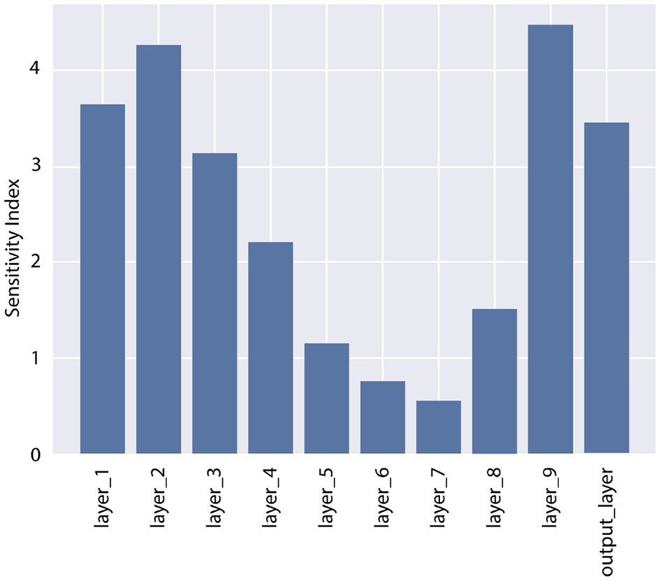
Sensitivity Index (SI) for all layers in the DNN for the test problem. Layer 9 has the highest SI and is selected for Bayesianization.
Our pBNN is implemented using TensorFlow Probability (TFP) (Dillon et al., 2017), where Layer 9 is replaced with a DenseFlipout layer and all other layers remaining to be Dense. Training is then performed simultaneously on θB and wD as in Equation 8. For the Bayesianized DNN parameters (wB), we adopt independent Gaussian priors with a rather wide standard deviation to reflect an initial uninformative distribution: . A Gaussian likelihood is also used to depict independent Gaussian observation noise (σϵ = 0.02 to be consistent with the data-generation in Equation 9) on the y targets:
The variational posteriors are from the family of independent Gaussians , and so the variational parameters are θ = {μi, σi}. We train this pBNN using the Nadam (Dozat, 2016) optimizer for 104 epochs with a learning rate of 10−3 and batch size of 64.
To assess whether the pBNN constructed with SA-selected Layer 9 provides a good approximation to the uncertainty of the full BNN, we also train a full BNN where all layers are replaced by DenseFlipout layers; the posterior push-forward uncertainty2 of the full BNN is shown in Figure 3. Furthermore, to investigate the performance of pBNNs if a layer different from Layer 9 were selected, we construct separate pBNNs where a different layer is Bayesianized.
Figure 3

Training data (black dots) overlaid with the deterministic DNN prediction (solid orange) and full BNN posterior push-forward uncertainty (solid blue line is the mean, blue shadow is the 95% credible interval).
Since a good pBNN is one that faithfully approximates the uncertainty in the full BNN, we measure its performance based on how close the pBNN's posterior push-forward is to the full BNN's posterior push-forward via the KL divergence. Following the same reasoning as the SI from Equation 6, we normalize this quantity by multiplying Nℓ (since lower KL is better), to arrive at our validation metric:
where are the Bayesianized parameters in the pBNN, and are the full set of parameters (all Bayesianized) in the full BNN. The Dnorm values for each pBNN are plotted against SI in Figure 4, where we observe a Spearman's correlation of rs = −0.83 which is considered to be strongly correlated in literature (Akoglu, 2018). This supports our SA-based layer selection strategy, where the layers with high SI will also lead to low Dnorm. Lastly, we note that while we perform this brute-force comparison to validate the effectiveness of our approach, in practice one would only train the pBNN on the SA-selected layer as described in Section 3.
Figure 4

Normalized KL divergence from the full BNN posterior push-forward to the different pBNNs is highly correlated with the SI that is used to select the layer for Bayesianization (Spearman's correlation rs = −0.83).
5. Demonstration: Tumor segmentation with U-Net
Here, we present the main demonstration of our pBNN, applying it to a state-of-the-art DNN model used for medical image segmentation: the U-Net (Ronneberger et al., 2015). Since our goal is to demonstrate our pBNN framework presented in Section 3 and not to develop or justify the choice of architecture, we take the U-Net architecture as given.
5.1. Step 1: Access a deterministic DNN model
We begin by training a U-Net deterministically using the architecture and code published by Ojika et al. (2020). As shown in Figure 5, the U-Net comprises of an encoder, decoder, and skip connections. The encoder module composes of 2D Convolutional layers followed by MaxPooling layers with window size 2 × 2, and 2D Spatial Dropout layers for regularization. The decoder module is composed of corresponding Conv2DTranspose layers followed by Concatenate layers. Nested in between the encoder and decoder is the 2D Upsampling layer with bilinear interpolation. The U-Net has feature map size set to 32, kernel size 3 × 3, and dropout rate 0.2. For the 2D Convolutional layers, ReLU activation is used along with He uniform variance scaling initializer, and kernel size is set to 2 × 2. Overall, this U-Net has a total of 7.8 million tunable parameters.
Figure 5

U-Net architecture with our naming system of the different tunable layers considered for the pBNN.
We perform the training on dataset from the Medical Segmentation Decathlon Challenge Task 01 (Simpson et al., 2019) consisting of brain MRI scans of patients with glioma. The training set contains of 58,464 2D images (each sized 144 × 144) and a separate validation set contains 6,624 images. Data augmentation is employed during training to increase data diversity including random choices of horizontal and vertical flips, ±45° rotation, and ±2.5° shearing. The ADAM optimizer (Kingma and Ba, 2015) is run for 30 epochs used a learning rate 0.001 and a mini-batch size of 128. The training loss function is a weighted sum of the Dice coefficient (Dice, 1945; Crum et al., 2006) and standard Binary Cross Entropy. The training results are summarized in Table 2.
Table 2
| Performance | Value |
|---|---|
| Training time | 5 h |
| Model size | 94.3 Mb |
| Trainable parameters | 7.8 million |
| Validation accuracy | 0.9915 |
| Validation dice coefficient | 0.8508 |
Summary of the deterministic U-Net training.
5.2. Step 2: Conduct sensitivity analysis to select a layer for Bayesian inference
We computed the gradient-based SI in Equation 6 for each candidate layers, shown in Figure 6. In particular, the layers near the top portion of the encoder carry larger SI. This response gradually decreases proceeding further into the model, reaching a minimum near the middle, followed by a light rebound at the decoder layers. The lowest SI occurs at Layer decoder_3a, and the highest SI is at Layer encoder_1a. Layer encoder_1a is therefore selected for Bayesianization.
Figure 6

Sensitivity Index (SI) for all layers in the U-Net used for tumor segmentation. The layer encoder_1a has the highest SI and is selected for Bayesianization.
5.3. Step 3: Perform targeted Bayesian inference to build pBNN
We construct a pBNN by performing Bayesian inference on encoder_1a using Flipout VI and training all other layers deterministically, following Equation 8. We implement our pBNN using TensorFlow Probability (TFP) (Dillon et al., 2017) by replacing the 2DConvolution layer of encoder_1a with tfp.layers.Convolution2DFlipout. Training is then performed simultaneously on θB and wD as in Equation 8. For the Bayesianized DNN parameters (wB), we adopt independent Gaussian priors with a rather wide standard deviation to reflect an initial uninformative distribution: . Since our data label for each pixel is binary while our model prediction ranges [0, 1], we adopt a likelihood associated with the binary cross entropy:
The variational posteriors are from the family of independent Gaussians , and so the variational parameters are θ = {μi, σi}. We train this pBNN using the Nadam (Dozat, 2016) optimizer for 400 epochs with a learning rate of 10−4 and batch size of 196, using 8 GeForce RTX 2080 Ti GPUs in parallel. The ELBO training history of the pBNN is shown in Figure 7 (plot with encoder_1a emphasized in red). While the plot indicates a small rise around 150 epochs due to numerical instabilities with the optimization algorithm, overall the curve steadies out by 350 epochs (note that the y-axis is logarithmic which amplifies the lower-value fluctuations) and appears noticeably flatter compared to the beginning of the optimization.
Figure 7

ΔELBO training history for all models.
6. Validation of the pBNN
In this section, we provide validation for the pBNN procedure, by illustrating whether the U-Net pBNN constructed with SA-selected encoder_1a layer provides a good approximation to the uncertainty of the full BNN. To achieve this, we also need to train a full BNN where Bayesian inference is performed on all layers. Such attempt to obtain the full uncertainty is highly expensive, and is in fact the original motivation for the new pBNN. We clarify that a full BNN is not needed as a part of the regular pBNN procedure described in Section 3.
We train the full BNN, where all 19 layers of the U-Net are Bayesianized, using the full extent of our available computational resources: 2000 epochs using the Nadam (Dozat, 2016) optimizer with learning rate 10−4 and batch size of 196, 94.72 GB of memory, 8 GPUs in parallel, and it required 3 days of continuous computation to arrive at a steadied ELBO. The best-performing model is saved during the training process. Due to the tremendous size of this BNN, expert experience is also relied upon for randomized initialization and algorithm tuning to arrive at a reasonably converged full BNN. Additionally, we also train the 19 pBNNs, each with one of the 19 layers targeted for Bayesian inference, but with shorter 400 epochs. The ELBO training history for all models are summarized in Figure 7, with the pBNN using the SA-selected layer (encoder_1a) emphasized in red. While we train the full BNN for significantly longer than the pBNNs, we plot their ELBO to around 350 epochs for better readability and comparison. All training curves gradually decrease and start flattening around 150 epochs, after which they become noisy. The plot suggests that all pBNN models we built have converged reasonably well.
Since a good pBNN is one that faithfully approximates the uncertainty in the full BNN, we measure the pBNN performance using the normalized KL divergence between the pBNN's posterior push-forward to the full BNN's posterior push-forward, Dnorm, defined in Equation 11.
With each U-Net output being a 144 × 144 pixel values, directly computing the KL divergence for the joint 144 × 144-dimensional posterior push-forward PDF would be very difficult. Therefore, we further simplify the computation of Dnorm through an independence approximation, breaking the 144 × 144-dimensional KL into 20,736 pixel-wise one-dimensional KL computations. For a given prediction image, each pixel's KL is estimated by first generating 100 samples of the DNN parameters wpartial, B from the optimized variational posterior , combine it with the other deterministic parameters and evaluate the corresponding pixel predictions , and for each pixel fit its 100 samples to a Beta distributions to approximate its posterior push-forward PDF. Beta distributions are often used to model the uncertainty of Bernoulli distributions and suitable for our problem to ensure pixel-wise prediction values reside between [0, 1]. Once the Beta PDFs are extracted, KL divergence can be calculated analytically. The pixel-wise KL divergence values are then summed to obtain the estimate to the joint PDF's KL value (since the KL divergence between two joint PDFs that are independent factors into the sum of KL divergences of individual marginals). The final Dnorm are shown in Figure 8, and they show a correlated, inverse trend compared to the SI values in Figure 6, supporting that SI is a good inexpensive indicator of the KL performance metric.
Figure 8

Normalized KL Dnorm, for all 19 pBNNs each built with Bayesian inference on one of the layers in the U-Net.
Figure 9 shows a scatter plot for all 19 pBNNs the KL divergence (not yet normalized by Nℓ) vs. Nℓ the number of parameters of the layer targeted for Bayesian inference; the pBNN with the SA-selected layer (encoder_1a) is marked in red. Ideally, we would like to select a layer for Bayesianization that has low KL divergence and small number of layer parameters (i.e., toward the bottom-left corner). However, these two desirable properties generally conflict and a tradeoff needs to be made. This can be seen by the Pareto optimality front by the plot's lower-left convext hull. In this case, we see our SA criterion indeed identifies one of the Pareto points in layer encoder_1a. The output_layer also resides on the Pareto, and would also serve as a reasonable selection for Bayesianization; indeed, the SI values presented in Figure 6 does show the output_layer to be the runner-up. However we point out that the nature of how the two layers are good choices are different: encoder_1a achieves a lower KL than output_layer, but output_layer has a smaller number of parameter.
Figure 9

Scatter plot of KL divergence sum vs. number of parameters in the Bayesian layer.
7. Looking toward uncertainty maps and their interpretation
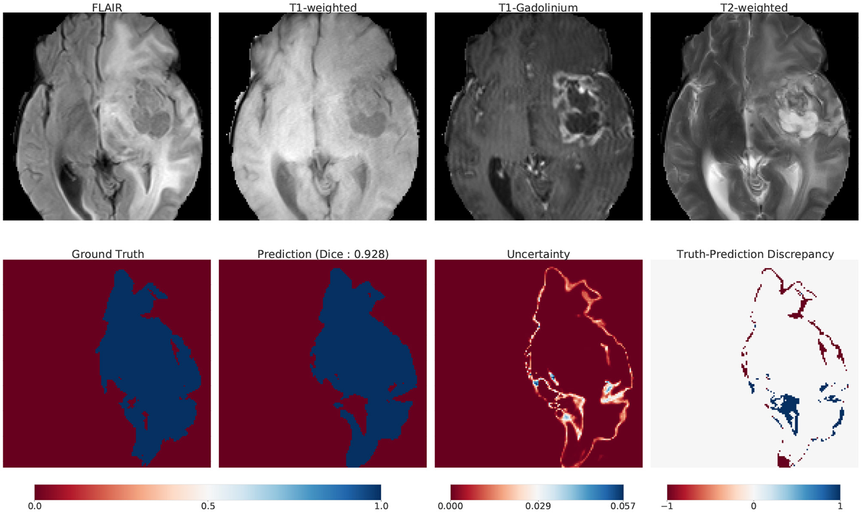
Although the main contribution of our work is to provide a scalable method for Bayesian UQ in large DNNs, here we illustrate one way that our uncertainty information could be used in practice. We introduce uncertainty maps as a tool that communicates how confident (uncertain) a model is in its prediction. Figure 10 illustrates these maps for one such example: top row displays the 4 modalities of MRI; bottom row displays the ground truth, prediction, uncertainty and truth-prediction discrepancy respectively for the SA-guided pBNN (Section 5.3).
Figure 10
Uncertainty map accompanying a prediction made by the pBNN.
7.1. Construction
We describe how we compute and visualize the uncertainty of the pBNN's prediction for a specific use case (Figure 10). We chose this image from our test dataset as an example because the ground truth indicated a large percent of the pixels belonging to the tumor class (25%). First, we obtain 100 samples from the posterior push-forward distribution of our trained pBNN for this MRI. To construct the prediction map, we take the mean of these 100 samples. We then map the continuous values [0,1] to their dominant class (tumor or non-tumor) with thresholding (value of 0.5).
We build the uncertainty map with the same 100 samples, by computing within-pixel standard deviation. The range of uncertainty displayed is unique to the image and is not a global uncertainty measure. To visualize the truth-prediction discrepancy map, we subtract the prediction map from the ground truth. The negative extreme value (−1) indicates regions where the model predicts tumor when the tumor is absent in ground truth (false positive, or over-prediction). The positive extreme value (+1) indicates regions where the model does not predict tumor when the tumor is present in the ground truth (false negative, or under-prediction).
7.2. Interpretation
We show a use-case scenario on how to interpret and analyze uncertainty maps. We asked one of the co-authors who is a researcher in radiation oncology, and a collaborator with routine knowledge of MRI image interpretation to conduct a preliminary interpretation and analysis of the MRI and the uncertainty map in Figure 10. Note that this interpretation was not performed by board-certified radiologists, so it only serves as a guiding example.
According to their interpretation, it was clear to them that the pBNN was fairly confident in distinguishing the tumor core from the background, but was highly uncertain at the boundary regions of the tumor. This is consistent with manual segmentation. For example, even when a single radiologist performs multiple segmentations on the same image, the most differences (intra-rater variability) are often present in the boundary region.
In this particular example, the necrosis, enhancing, and non-enhancing parts of the tumor are surrounded by edema. Since the model predicts the whole tumor and does not perform subclass recognition, it predicts the edematous region of the tumor. However, since edema has a distinct contrast in FLAIR, there is a possibility that this FLAIR modality is contributing largely to the observed uncertainty. This is in line with segmentation by radiologists, which also has the most uncertainty in FLAIR modality.
Further, comparing the uncertainty map with the truth-prediction discrepancy revealed that the pBNN is highly uncertain where it under-predicts and had low uncertainty where it over-predicts. A possible reason for this is in the context of the model's ability to correctly call out all of the tumor pixels in the ground truth. For over-prediction, the model covered the tumor region and went beyond it (which does not count as a “miss”), so the uncertainty is low. Whereas for under-prediction, the model failed to correctly call out tumor (which counts as a “miss”), thus the uncertainty is high. One such area of under-prediction is in the lateral ventricle of the right hemisphere. This region is darker than the rest of the tumor (in FLAIR modality), but is still a part of the tumor due to the presence of edema.
One possible explanation of this model behavior is that the model has learned to distinguish tumors based on pixel intensity and contrast. As the algorithm “sees” the lateral ventricle of the right hemisphere to be significantly darker than the rest of the tumor, it thinks this is not a tumor. While this seems like a reasonable mistake for the model to make, a radiologist would have no problem marking this as a tumor as they have a firm understanding of anatomy. Example regions of over-prediction are near the middle frontal gyrus and near the necrotic region in the right hemisphere. This region is craggy, and it seems like the model smoothed over these intricacies to get a “good enough” prediction.
8. Discussion
The results of our empirical validation in Section 6 illustrate the effectiveness of the pBNN: the pBNN where Bayesian inference is performed on the SA-selected layer achieves the lowest normalized KL divergence—that is, compared to if a different layer were chosen, it provides the best capturing of the full BNN uncertainty. Our three-step pBNN methodology in Section 3 is set up with implementation considerations in mind. Step 1 allows the leveraging of pre-existing trained DNNs, but also describes the procedure if a new DNN needs to be trained from scratch. Step 2 assesses and identifies the portion of DNN for Bayesian inference on a layer-by-layer basis (i.e., keeping “layer” as the unit), since accessing and replacing an entire layer (e.g., from a Dense layer to DenseFlipout layer) is very convenient in programming infrastructure such as TensorFlow Probability. Such modifications do not need the user to program new layers, or to Bayesianize portions of a layer. The gradient-based sensitivity measure adopted is also inexpensive to compute and can be readily extracted from a deterministic DNN. Step 3 takes advantage of existing implementations of Bayesian inference algorithms, such as the Flipout VI that can be specified and used together with non-Bayesian layers.
Our method is particularly valuable for high-dimensional problems (e.g., DNNs with millions of parameters), where performing a full Bayesian inference would be extremely expensive. Our work enables principled approximate Bayesian inference to be scaled up to millions of dimensions. While other related partial Bayesian strategies compare test error performance (Zeng et al., 2018), we explicitly compute closeness to the fully Bayesian model, with the aim of faithfully capturing the true uncertainty that we are justified to have. Our overarching goal is provide a transparent quantification of uncertainty of our AI system (not to only optimize accuracy).
We illustrate how our computational framework could be used to visually represent prediction uncertainty in Section 7. While uncertainty communication is not the primary goal of our paper, we demonstrate how our work can advance an understanding of AI in a healthcare context. We conduct preliminary analysis on these maps to demonstrate how a radiologist might interpret these images. The maps allow one to correlate the model's mistakes and how confidently the model fails. With clinical insights and interpretation, one can also explore the model's behavior on specific use cases. For example, model predictions on out-of-distribution data can be potentially flagged based on uncertainty (Ovadia et al., 2019) to caution the radiologist about model's reliability in those regions. This would be especially useful for healthcare contexts where models are highly domain-dependent and localized (Finlayson et al., 2021). Apart from it's potential to enable flagging of unreliable cases, our Bayesian framework can allow for construction of an expert-informed pBNN. It permits a flexible choice for prior and likelihood, potentially allowing practitioners to inject their specialized knowledge. For this, we refer to a branch of Bayesian statistics called expert knowledge elicitation (O'Hagan et al., 2006).
While our work produced promising results, limitations still exist. While we provided a detailed validation by brute-force computation of the full BNN, one would not do so in practice. Assessing the quality of posterior approximation is a challenge in general for all BNNs, where inexpensive and effective diagnostics are needed to monitor the algorithm progress especially for large models. Analyzing ELBO curves is one such approach, but one cannot know when the ELBO is stuck in a local minimum. Furthermore, the magnitude of ELBO value does not directly indicate how far the variational approximation is to the true posterior, since ELBO differs from the KL divergence by an unknown constant (i.e., one should not expect ELBO does not converge toward zero with more epochs, as one would with mean-squared-error). We also have not explored performing Bayesian inference on multiple layers, or portions of layers, which may offer further improvements. Such expansions would require the development of efficient strategies to optimize SI across various combinations of multiple layers, and additional benchmarking and validation to assess the tradeoffs between their computational cost and ability to approximate the full BNN. Despite these limitations, our work demonstrates the effectiveness of SA-based pBNN in Bayesian UQ of large, million-dimensional DNNs.
9. Conclusion and future work
In this paper, we proposed an approach to compute the Bayesian uncertainty of million-dimensional DNNs for medical image segmentation. Starting from a deterministic DNN, we used gradient-based sensitivity analysis to identify a layer to perform Bayesian inference, thereby creating a partially Bayesian neural network (pBNN) that is computationally much less expensive to construct than a full BNN. We demonstrated the pBNN method on state-of-the-art 7.8-million parameter U-Net for brain tumor segmentation. Our validation indicated that the pBNN based on SA-selected layer provided the best approximation to the uncertainty from a full BNN, compared to other layer choices.
Our methodology enables model developers and practitioners to compute the Bayesian uncertainty for large deep learning models. In a life-critical domain such as healthcare, deep learning models can have far-reaching impact, but also can make mistakes leading to disastrous consequences. Communicating uncertainty in model predictions help encourage clinicians to engage with the AI-based DSS with a healthy dose of skepticism and failure-centric mindset. Additionally, UQ mitigate “super-human” perceptions of AI that can lead to unjustified over-reliance. Thus, quantifying and communicating uncertainty would allow for safer and responsible deployments of AI-based CDSS in clinical workflows.
For future work, we plan to conduct a large scale evaluation of the impact of uncertainty communication to radiologists for the task of tumor segmentation. In this paper, we conduct preliminary interpretation of these maps and demonstrate the possibility of such a study. We would further like to understand if these maps can be used as a tool for model explanation, and whether these maps are more useful than conventional metrics. It can also be a useful tool in reducing alarm and click fatigue, as the model can only predict when absolutely certain, and refrain from predicting otherwise.
Statements
Data availability statement
Publicly available datasets were analyzed in this study. This data can be found here: https://www.med.upenn.edu/cbica/sbia/brats2018/tasks.html.
Author contributions
JH: primarily conduct experiments and setting up Bayesian inference with test problem and U-Net. SP: data acquisition and pre-processing. SP and JH: Bayesian and deterministic model training and data analysis for U-Net. AR, NB, and XH: advising and supervision. All authors contributed to the conception of ideas, design of experiments, interpretation of results, and writing the manuscript. All authors contributed to the article and approved the submitted version.
Funding
SP, XH, and AR were partially supported by the University of Michigan (UM) Michigan Institute for Computational Discovery and Engineering (MICDE) Catalyst Grant Enabling Tractable Uncertainty Quantification for High-Dimensional Predictive AI Systems in Computational Medicine. AR was supported by CCSG Bioinformatics Shared Resource 5 P30 CA046592, a Research Scholar Grant from the American Cancer Society (RSG-16-005-01), and a UM Precision Health Investigator Award to AR (along with L. Rozek and M. Sartor). SP and AR were also partially supported by the NCI Grant R37-CA214955. JH, XH, and NB were supported in part by the U.S. Department of Energy, Office of Science, Office of Advanced Scientific Computing Research, under Award Numbers DE-SC0021397 and DE-SC0021398. This paper was prepared as an account of work sponsored by an agency of the United States Government. Neither the United States Government nor any agency thereof, nor any of their employees, makes any warranty, express or implied, or assumes any legal liability or responsibility for the accuracy, completeness, or usefulness of any information, apparatus, product, or process disclosed, or represents that its use would not infringe privately owned rights. Reference herein to any specific commercial product, process, or service by trade name, trademark, manufacturer, or otherwise does not necessarily constitute or imply its endorsement, recommendation, or favoring by the United States Government or any agency thereof. The views and opinions of authors expressed herein do not necessarily state or reflect those of the United States Government or any agency thereof.
Acknowledgments
Experiments were performed on Armis2 HPC Clusters provided by UM's Precision Health Initiative. Advice on clinical perspective on gliomas was provided by Dr. Danielle Bitterman and Nicholas Wang. Additionally, we thank Santhoshi Krishnan, Jane Im, and Sumit Asthana for providing valuable editing feedback.
Conflict of interest
AR serves as member for Voxel Analytics LLC. The remaining authors declare that the research was conducted in the absence of any commercial or financial relationships that could be construed as a potential conflict of interest.
Publisher’s note
All claims expressed in this article are solely those of the authors and do not necessarily represent those of their affiliated organizations, or those of the publisher, the editors and the reviewers. Any product that may be evaluated in this article, or claim that may be made by its manufacturer, is not guaranteed or endorsed by the publisher.
Footnotes
1.^Note that p(w|xT) = p(w), i.e., the prior uncertainty should not change from knowing only the input values of the training data without their output values.
2.^Posterior push-forward is p(f(x; wB, wD)|x, xT, yT), which differs from the posterior predictive p(y|x, xT, yT).
References
1
AkogluH. (2018). User's guide to correlation coefficients. Turk. J. Emerg. Med.18, 91–93. 10.1016/j.tjem.2018.08.001
2
AmershiS. (2020). “Toward responsible ai by planning to fail,” in Proceedings of the 26th ACM SIGKDD International Conference on Knowledge Discovery and Data Mining, KDD '20 (New York, NY: Association for Computing Machinery), 3607. 10.1145/3394486.3409557
3
AndrieuC.de FreitasN.DoucetA.JordanM. I. (2003). An introduction to MCMC for machine learning. Mach. Learn.50, 5–43. 10.1023/A:1020281327116
4
ArnoldM.BellamyR. K. E.HindM.HoudeS.MehtaS.MojsilovicA.et al. (2018). Factsheets: increasing trust in AI services through supplier's declarations of conformity. IBM J. Res. Dev.63, 6–1. 10.48550/arXiv.1808.07261
5
AzizzadenesheliK.BrunskillE.AnandkumarA. (2018). “Efficient exploration through Bayesian deep Q-networks,” in 2018 Information Theory and Applications Workshop, ITA 2018. 10.1109/ITA.2018.8503252
6
BegoliE.BhattacharyaT.KusnezovD. (2019). The need for uncertainty quantification in machine-assisted medical decision making. Nat. Mach. Intell.1, 20–23. 10.1038/s42256-018-0004-1
7
BenjamensS.DhunnooP.MeskóB. (2020). The state of artificial intelligence-based FDA-approved medical devices and algorithms: an online database. NPJ Digital Med.3, e324. 10.1038/s41746-020-00324-0
8
BergerJ. O. (1985). Statistical Decision Theory and Bayesian Analysis. Springer Series in Statistics.New York, NY: Springer. 10.1007/978-1-4757-4286-2
9
BernardoJ. M.SmithA. F. M. (2000). Bayesian Theory. New York, NY: John Wiley and Sons.
10
BetancourtM. (2017). A conceptual introduction to Hamiltonian Monte Carlo. arXiv [preprint] arXiv:1701.02434. 10.3150/16-BEJ810
11
BhattU.AntoránJ.ZhangY.LiaoQ. V.SattigeriP.FogliatoR.et al. (2021). “Uncertainty as a form of transparency: measuring, communicating, and using uncertainty,” in Proceedings of the 2021 AAAI/ACM Conference on AI, Ethics, and Society, AIES '21 (New York, NY: Association for Computing Machinery), 401–413. 10.1145/3461702.3462571
12
BleekerF. E.MolenaarR. J.LeenstraS. (2012). Recent advances in the molecular understanding of glioblastoma. J. Neuro-oncol.108, 11–27. 10.1007/s11060-011-0793-0
13
BleiD. M.KucukelbirA.McAuliffeJ. D. (2017). Variational inference: a review for statisticians. J. Am. Stat. Assoc.112, 859–877. 10.1080/01621459.2017.1285773
14
BlundellC.CornebiseJ.KavukcuogluK.WierstraD. (2015). “Weight uncertainty in neural networks,” in Proceedings of the 32nd International Conference on Machine Learning, volume 37, 1613–1622.
15
BowlerR. D.BachB.PschetzL. (2022). “Exploring uncertainty in digital scheduling, and the wider implications of unrepresented temporalities in HCI,” in Proceedings of the 2022 CHI Conference on Human Factors in Computing Systems, CHI '22 (New York, NY: Association for Computing Machinery). 10.1145/3491102.3502107
16
BrooksS.GelmanA.JonesG.MengX.-L. (eds). (2011). Handbook of Markov Chain Monte Carlo. London: Chapman and Hall. 10.1201/b10905
17
BussoneA.StumpfS.O'SullivanD. (2015). “The role of explanations on trust and reliance in clinical decision support systems,” in 2015 International Conference on Healthcare Informatics, 160–169. 10.1109/ICHI.2015.26
18
CampoloA.CrawfordK. (2020). Enchanted determinism: power without responsibility in artificial intelligence. Engag. Sci. Technol. Soc.6, 1–19. 10.17351/ests2020.277
19
CrumW.CamaraO.HillD. (2006). Generalized overlap measures for evaluation and validation in medical image analysis. IEEE Trans. Med. Imag.25, 1451–1461. 10.1109/TMI.2006.880587
20
DiceL. R. (1945). Measures of the amount of ecologic association between species. Ecology26, 297–302. 10.2307/1932409
21
DillonJ. V.LangmoreI.TranD.BrevdoE.VasudevanS.MooreD.et al. (2017). Tensorflow distributions. arXiv [preprint]. arXiv:1711.10604.
22
DozatT. (2016). “Incorporating Nesterov momentum into Adam,” in ICLR Workshop.
23
FerlayJ.ShinH. R.BrayF.FormanD.MathersC.ParkinD. M. (2010). Estimates of worldwide burden of cancer in 2008: Globocan 2008. Int. J. Cancer127, 2893–2917. 10.1002/ijc.25516
24
FinlaysonS. G.SubbaswamyA.SinghK.BowersJ.KupkeA.ZittrainJ.et al. (2021). The clinician and dataset shift in artificial intelligence. New Engl. J. Med.385, 283–286. 10.1056/NEJMc2104626
25
GalY. (2016). Uncertainty in Deep Learning (PhD thesis). University of Cambridge, Cambridge.
26
GhassemiM.NaumannT.SchulamP.BeamA. L.RanganathR. (2018). Opportunities in machine learning for healthcare. CoRR abs/1806.00388.
27
GhoshS.LiaoQ. V.Natesan RamamurthyK.NavratilJ.SattigeriP.VarshneyK.et al. (2022). “Uncertainty quantification 360: a hands-on tutorial,” in 5th Joint International Conference on Data Science Management of Data (9th ACM IKDD CODS and 27th COMAD), CODS-COMAD 2022 (New York, NY: Association for Computing Machinery), 333-335. 10.1145/3493700.3493767
28
GravesA. (2011). “Practical variational inference for neural networks,” in Advances in Neural Information Processing Systems 24 (NIPS 2011) (Granada, Spain), 2348–2356.
29
GriffithsF.GreenE.TsouroufliM. (2005). The nature of medical evidence and its inherent uncertainty for the clinical consultation: qualitative study. BMJ330, 511. 10.1136/bmj.38336.482720.8F
30
HaqueI. R. I.NeubertJ. (2020). Deep learning approaches to biomedical image segmentation. Inform. Med.18, 100297. 10.1016/j.imu.2020.100297
31
HastingsW. (1970). Monte Carlo sampling methods using Markov chains and their applications. Biometrika57, 97–109. 10.1093/biomet/57.1.97
32
HavaeiM.DavyA.Warde-FarleyD.BiardA.CourvilleA.BengioY.et al. (2017). Brain tumor segmentation with deep neural networks. Med. Image Anal.35, 18–31. 10.1016/j.media.2016.05.004
33
HesamianM. H.JiaW.HeX.KennedyP. (2019). Deep learning techniques for medical image segmentation: achievements and challenges. J. Digital Imag.32, 582–596. 10.1007/s10278-019-00227-x
34
HoffmanM. D.GelmanA. (2014). The no-u-turn sampler: adaptively setting path lengths in hamiltonian monte carlo. J. Mach. Learn. Res.15, 1593–1623.
35
JacobsM.HeJ.F. PradierM.LamB.AhnA. C.McCoyT. H.et al. (2021). “Designing ai for trust and collaboration in time-constrained medical decisions: a sociotechnical lens,” in Proceedings of the 2021 CHI Conference on Human Factors in Computing Systems, CHI '21 (New York, NY: Association for Computing Machinery). 10.1145/3411764.3445385
36
JordanM. I.JaakkolaT. S.SaulL. K.ParkF. (1999). An introduction to variational methods for graphical models an introduction to variational methods for graphical models. Mach. Learn.37, 183–233.
37
KausM. R.WarfieldS. K.NabaviA.BlackP. M.JoleszF. A.KikinisR. (2001). Automated segmentation of mr images of brain tumors. Radiology218, 586–591. 10.1148/radiology.218.2.r01fe44586
38
KingmaD. P.BaJ. (2015). “Adam: a method for stochastic optimization,” in 3rd International Conference on Learning Representations, ICLR 2015 (San Diego, CA).
39
KocherM.RugeM. I.GalldiksN.LohmannP. (2020). Applications of radiomics and machine learning for radiotherapy of malignant brain tumors. Strahlenther. Onkol.196, 856–867. 10.1007/s00066-020-01626-8
40
KrishnanR.SubedarM.TickooO. (2020). “Specifying weight priors in bayesian deep neural networks with empirical bayes,” in Proceedings of the AAAI Conference on Artificial Intelligence, 4477–4484. 10.1609/aaai.v34i04.5875
41
LeCunY. A.BottouL.OrrG. B.MüllerK.-R. (2012). “Efficient BackProp,” in Neural Networks: Tricks of the Trade, eds G. Montavon, G. B. Orr, and K.-R. Müller (Berlin: Springer Heidelberg), 9–48. 10.1007/978-3-642-35289-8_3
42
LeibigC.AllkenV.AyhanM. S.BerensP.WahlS. (2017). Leveraging uncertainty information from deep neural networks for disease detection. Sci. Rep.7, 17876. 10.1038/s41598-017-17876-z
43
MacKayD. J. C. (1992). A practical Bayesian framework for backpropagation networks. Neural Comput.4, 448–472. 10.1162/neco.1992.4.3.448
44
MitchellM.WuS.ZaldivarA.BarnesP.VassermanL.HutchinsonB.et al. (2019). “Model cards for model reporting,” in Proceedings of the Conference on Fairness, Accountability, and Transparency, FAT* '19 (New York, NY: Association for Computing Machinery), 220-229. 10.1145/3287560.3287596
45
NazarU.KhanM. A.LaliI. U.LinH.AliH.AshrafI.et al. (2020). Review of automated computerized methods for brain tumor segmentation and classification. Curr. Med. Imag.16, 823–834. 10.2174/1573405615666191120110855
46
NealR. M. (1996). Bayesian Learning for Neural Networks. New York, NY: Springer-Verlag. 10.1007/978-1-4612-0745-0
47
NealR. M. (2011). “MCMC using Hamiltonian dynamics,” in Handbook of Markov Chain Monte Carlo, 113–162. 10.1201/b10905-6
48
O'HaganA.BuckC. E.DaneshkhahA.EiserJ. R.GarthwaiteP. H.JenkinsonD. J.et al. (2006). Uncertain Judgements: Eliciting Experts' Probabilities. Chichester: John Wiley and Sons. 10.1002/0470033312
49
OjikaD.PatelB.ReinaG. A.BoyerT.MartinC.ShahP. (2020). Addressing the memory bottleneck in AI model training. arXiv [preprint]. arxiv:2003.08732. 10.48550/arXiv.2003.08732
50
OvadiaY.FertigE.RenJ.NadoZ.SculleyD.NowozinS.et al. (2019). “Can you trust your model's uncertainty? evaluating predictive uncertainty under dataset shift,” in Advances in Neural Information Processing Systems, vol. 32, eds H. Wallach, H. Larochelle, A. Beygelzimer, F. d'Alché-Buc, E. Fox, and R. Garnett (New York, NY: Curran Associates, Inc).
51
PapernotN.McDanielP. D.GoodfellowI. J. (2016). Transferability in machine learning: from phenomena to black-box attacks using adversarial samples. CoRR. abs/1605.07277.
52
PushkarnaM.ZaldivarA.KjartanssonO. (2022). Data cards: purposeful and transparent dataset documentation for responsible AI. arXiv [preprint]. arXiv:2204.01075. 10.1145/3531146.3533231
53
RajpurkarP.ChenE.BanerjeeO.TopolE. J. (2022). AI in health and medicine. Nat. Med.28, 31–38. 10.1038/s41591-021-01614-0
54
RiquelmeC.TuckerG.SnoekJ.BrainG. (2017). “Deep Bayesian bandits showdown,” in NIPS 2017 Bayesian Deep Learning Workshop.
55
RobbinsH.MonroS. (1951). A stochastic approximation method. Ann. Math. Stat.22, 400–407. 10.1214/aoms/1177729586
56
RobertC. P.CasellaG. (2004). Monte Carlo Statistical Methods. New York, NY: Springer New York. 10.1007/978-1-4757-4145-2
57
RonnebergerO.FischerP.BroxT. (2015). “U-Net: Convolutional Networks for Biomedical Image Segmentation,” in Medical Image Computing and Computer-Assisted Intervention—MICCAI 2015—18th International Conference Munich, Germany, October 5-9, 2015, Proceedings, Part III, volume 9351 of Lecture Notes in Computer Science (New York, NY: Springer Verlag), 234–241. 10.1007/978-3-319-24574-4_28
58
SimpsonA. L.AntonelliM.BakasS.BilelloM.FarahaniK.Van GinnekenB.et al. (2019). A large annotated medical image dataset for the development and evaluation of segmentation algorithms. arXiv [preprint] arXiv:1902.09063.
59
SiviaD. S.SkillingJ. (2006). Data Analysis: A Bayesian Tutorial, 2nd edition. New York, NY: Oxford University Press.
60
StricklandE. (2019). IBM Watson, heal thyself: How IBM overpromised and underdelivered on ai health care. IEEE Spect.56, 24–31. 10.1109/MSPEC.2019.8678513
61
StroomJ. C.HeijmenB. J. (2002). Geometrical uncertainties, radiotherapy planning margins, and the ICRU-62 report. Radiother. Oncol.64, 75-83. 10.1016/S0167-8140(02)00140-8
62
StuppR.MasonW. P.Van Den BentM. J.WellerM.FisherB.TaphoornM. J.et al. (2005). Radiotherapy plus concomitant and adjuvant temozolomide for glioblastoma. New Engl. J. Med.352, 987–996. 10.1056/NEJMoa043330
63
TonekaboniS.JoshiS.McCraddenM. D.GoldenbergA. (2019). “What clinicians want: Contextualizing explainable machine learning for clinical end use,” in Proceedings of the 4th Machine Learning for Healthcare Conference, volume 106 of Proceedings of Machine Learning Research, eds F. Doshi-Velez, J. Fackler, K. Jung, D. Kale, R. Ranganath, B. Wallace, et al. (Ann Arbor, MI: PMLR), 359–380.
64
TopolE. J. (2019). High-performance medicine: the convergence of human and artificial intelligence. Nat. Med.25, 44–56. 10.1038/s41591-018-0300-7
65
TsagkarisC.PapazoglouA.MoysidisD.PapadakisM.TrompoukisC. (2022). Bayesian versus frequentist clinical research now and then: lessons from the greco-roman medical scholarship. Ethics Med. Public Health23, 100805. 10.1016/j.jemep.2022.100805
66
Valentin JospinL.BuntineW.BoussaidF.LagaH.BennamounM. (2020). Hands-on Bayesian neural networks-a tutorial for deep learning users. arXiv [preprint] arXiv-2007.
67
VayenaE.BlasimmeA.CohenI. G. (2018). Machine learning in medicine: addressing ethical challenges. PLoS Med. 15, e1002689. 10.1371/journal.pmed.1002689
68
WainwrightM. J.JordanM. I. (2007). Graphical models, exponential families, and variational inference. Found. Trends Mach. Learn.1, 1–305. 10.1561/2200000001
69
WangD.MaesP.RenX.ShneidermanB.ShiY.WangQ. (2021). “Designing ai to work with or for people?,” in Extended Abstracts of the 2021 CHI Conference on Human Factors in Computing Systems, CHI EA '21 (New York, NY: Association for Computing Machinery). 10.1145/3411763.3450394
70
WenY.VicolP.BaJ.TranD.GrosseR. (2018). Flipout: efficient pseudo-independent weight perturbations on mini-batches. arXiv [preprint] arXiv:1803.04386.
71
ZengJ.LesnikowskiA.AlvarezJ. M. (2018). The relevance of Bayesian layer positioning to model uncertainty in deep Bayesian active learning. arXiv [preprint] arXiv:1811.12535.
Summary
Keywords
medical decision-making, Bayesian uncertainty, Responsible AI, transparency, tumor segmentation
Citation
Prabhudesai S, Hauth J, Guo D, Rao A, Banovic N and Huan X (2023) Lowering the computational barrier: Partially Bayesian neural networks for transparency in medical imaging AI. Front. Comput. Sci. 5:1071174. doi: 10.3389/fcomp.2023.1071174
Received
15 October 2022
Accepted
13 January 2023
Published
15 February 2023
Volume
5 - 2023
Edited by
Renwen Zhang, National University of Singapore, Singapore
Reviewed by
Lihong He, IBM, United States; Ziwei Liu, Nanyang Technological University, Singapore
Updates
Copyright
© 2023 Prabhudesai, Hauth, Guo, Rao, Banovic and Huan.
This is an open-access article distributed under the terms of the Creative Commons Attribution License (CC BY). The use, distribution or reproduction in other forums is permitted, provided the original author(s) and the copyright owner(s) are credited and that the original publication in this journal is cited, in accordance with accepted academic practice. No use, distribution or reproduction is permitted which does not comply with these terms.
*Correspondence: Snehal Prabhudesai ✉ snehalbp@umich.edu
†These authors share first authorship
This article was submitted to Human-Media Interaction, a section of the journal Frontiers in Computer Science
Disclaimer
All claims expressed in this article are solely those of the authors and do not necessarily represent those of their affiliated organizations, or those of the publisher, the editors and the reviewers. Any product that may be evaluated in this article or claim that may be made by its manufacturer is not guaranteed or endorsed by the publisher.