Quantum image denoising: a framework via Boltzmann machines, QUBO, and quantum annealing

1. Introduction

Quantum annealing (QA) (Kadowaki and Nishimori, 1998; Das and Chakrabarti, 2008; Albash and Lidar, 2018) is a promising technology for obtaining good solutions to difficult optimization problems, by making use of quantum interactions to aim to solve Ising or quadratic unconstrained binary optimization (QUBO) instances. Since Ising and QUBO instances are NP-hard, and many other combinatorial optimization problems can be reformulated as Ising or QUBO instances (see e.g., Glover et al., 2018), QA has the potential to become an extremely useful tool for optimization. As the capacities of commercially available quantum annealers continue to improve rapidly, it is of great interest to build models that are well-suited for this emerging technology. Furthermore, QA has promising machine learning applications surrounding Boltzmann Machines (BMs), as both QA and BMs are closely connected to the Boltzmann distribution. Boltzmann Machines are a type of generative artificial neural network that aim to learn the distribution of some training data set by fitting a Boltzmann distribution to the data, as described thoroughly in (Goodfellow et al., 2016, §20). On the other hand, QA aims to produce approximate minimum energy (maximum likelihood) solutions to a Boltzmann distribution via finding the ground state of the associated Hamiltonian that determines the distribution. Hence, maximum likelihood type problems on BMs are a natural candidate for applying QA in a machine learning framework. We contribute to the goal of furthering useful applications of QA in machine learning in this paper by building an image denoising model particularly well-suited for implementation via QA.

The task of image denoising is a fundamental problem in image processing and machine learning. In any means of collecting images, there is always a chance of some pixels being afflicted by noise that we wish to remove; see e.g., Boyat and Joshi (2015) for a good overview. Accordingly, many classical and data-driven approaches to the image denoising problem have been studied in the literature (Greig et al., 1989; Rudin et al., 1992; Buades et al., 2005; Tang et al., 2012; Cho, 2013). This paper studies a quantum binary image denoising model using Restricted Boltzmann Machines (RBMs henceforth) (Goodfellow et al., 2016, §20.2) that can take advantage of QA by formulating the denoising problem as a QUBO instance. Specifically, given a trained RBM, we introduce a penalty-based denoising scheme that admits a simple QUBO form, for which we derive the statistically optimal penalty parameter as well as a practically-motivated robustness modification. The denoising step only needs to solve a QUBO admitting a bipartite graph representation, and so is well-suited for QA. As QA has also shown promise for training BMs (Adachi and Henderson, 2015; Dixit et al., 2021), our full model lends itself well for denoising images using quantum annealers, and could thus play a role in the their future applications since QA can then be leveraged for both the training and denoising steps. The model also shows promise in absence of QA, and our insights presented are not limited to the QA framework, as the QUBO formulation of the denoising problem and its statistical properties we prove may be of independent interest.

The paper is organized as follows. Section 2 gives a summary of background on quantum annealing and Boltzmann Machines. Section 3 describes our main contribution of the image denoising model for QAs, and Section 4 shows some practical results obtained.

Remark 1.1. We frame our work as a binary image denoising method, although the framework does not depend on the data being images, and can be applied to the denoising of any binary data. This is because the framework does not use any spatial relationships between the pixels, and instead treats the image as a flattened vector whose distribution is to be learned. Hence, the denoising scheme can be applied as-is to any other binary data setting.

1.1. Contributions and organization

We provide QUBO-based denoising method for binary images (applicable to general binary data) using restricted Boltzmann machines in Section 3. This is done by formulating the denoising objective in equation 6 by combining the energy function of the distribution learned by the RBM with a (parameterized) penalty term for deviations from a given noisy image. This objective turns out to have an equivalent QUBO formulation, which is shown in claim 1. In Theorem 3.4, we derive the optimal choice for the penalty parameter under the assumption that the true images follow the distribution learned by the RBM, which also recovers the maximum a posteriori estimate per Corollary 3.5, though our model is more flexible, and this flexibility allows for useful practical modifications. Theorem 3.6 shows that the denoising method yields a result that is strictly closer (in expectation) to the true image than the noisy image is, under some additional assumptions. Given that these idealistic assumptions won't be met in reality, we propose a robustness modification in Section 3.3 that improves performance empirically. In Section 4, as the method lends itself well to quantum annealing, we then implement the method on a D-Wave Advantage 5000-qubit quantum annealer, demonstrating strong empirical performance. Since only small datasets can be tested on the D-Wave machine due to the relatively low number of qubits, we also test the method on a larger dataset, for which we use simulated annealing on a conventional computer in place of quantum annealing to find good solutions the QUBO denoising objective. Though we highlight the method being well-suited for quantum annealers, we emphasize that it may be of independent interest to the machine learning and image processing communities at large.

1.2. Related work

Closely related work of Koshka and Novotny (2021) uses a similar model as ours for the image reconstruction task, also solving QUBO formulations via quantum annelaing. In the reconstruction task, some subset of pixels is unknown (or obscured or missing), and needs to be restored, whereas our work considers denoising, where which pixels are noise-afflicted is unknown. Greig et al. (1989) derives a maximum a posteriori (MAP) estimator for the noise free image as a denoising method in a particular model of binary images that is less general than ours, though we would recover their estimator under a particular choice of our penalty parameter if we were to apply our framework to their model (since we recover MAP in a more general setting). Further, RBMS and quantum annealing have been studied for the classification problem, for instance in Adachi and Henderson (2015) and Krzysztof et al. (2021). Other research in the machine learning communities has also studied handling label noise, such as related work in Vahdat (2017), which studies the problem of training models in the presence of noisy labels, whereas our approach is entirely unsupervised (the data need not have any labels to begin with).

2. Background

Quantum Annealers make use of quantum interactions with the primary goal of finding the ground state of Hamiltonian by initializing and then evolving a system of coupled qubits over time (Johnson et al., 2011). In particular, we may view QA as implementing the Ising spin-glass model (Nishimori, 2001) evolving over time. As the QUBO model is equivalent to the Ising model (Glover et al., 2018), and QUBO instances can be efficiently transformed to Ising instances, a QA is well suited to provide good solutions to QUBO problems. A QUBO cost function, or energy function, takes the form

$\begin{array}{ll}{f}_Q(x):={\displaystyle \sum _{i,j}}{Q}_{ij}{x}_i{x}_j& (1)\end{array}$

where x_i ∈ {0, 1}, and Q is a symmetric, real-valued matrix. We will occasionally refer to Q_ij as the weight between x_i and x_j. QUBO is well-known to be NP hard (Barahona, 1982), and many combinatorial problems can be reformulated as QUBO instances. See Lucas (2014) and Glover et al. (2018) for thorough presentation of QUBO formulations of various problems. A Boltzmann Distribution using the above QUBO as its energy function takes the form

$\begin{array}{ll}{P}_Q^{model}(x)=\frac{1}{z}exp(-f_Q(x)),& (2)\end{array}$

where z is a normalizing constant. Note that a parameter called inverse temperature has been fixed to unity and is not explicitly shown in the above expression. In this paper, we will focus on making use of Boltzmann Machines, a type of generative neural network that fits a Boltzmann Distribution to the training data via making use of latent variables. Specifically, we consider Restricted Boltzmann Machines (RBMs), which have seen significant success and frequent use in deep probabilistic models (Goodfellow et al., 2016). RBMs consist of an input layer of visible nodes, and a layer of latent, or hidden nodes, which each have zero intra-group weights. Let v ∈ {0, 1}^v and h ∈ {0, 1}^h denote the visible and hidden nodes, respectively. It will be convenient for us to write x = (v, h) ∈ {0, 1}^v+h as their concatenation. The probability distribution represented by a RBM is then

$\begin{array}{ll}{P}_Q^{model}((\text{v},\text{h}))=\frac{1}{z}exp(-f_Q(\text{v},\text{h}))& (3)\end{array}$

with the restriction that Q_ij = Q_ji = 0 if i, j ∈ {1, …, v} or i, j ∈ {v + 1, …, v + h}. Hence, we have the simplified energy function

$\begin{array}{l}f((\text{v},\text{ h}),Q)={\displaystyle \sum _{i=1}^{v+h}}{\displaystyle \sum _{j=1}^{v+h}}2Q_{ij}{(\text{v},\text{ h})}_i{(\text{v},\text{ h})}_j={\displaystyle \sum _{i=1}^v}{\displaystyle \sum _{j=v+1}^{v+h}}{Q}_{ij}{\text{v}}_i{\text{h}}_j\\ +{\displaystyle \sum _{i=1}^v}{Q}_{ii}{\text{v}}_i^2+{\displaystyle \sum _{i=v+1}^{v+h}}{Q}_{ii}{\text{h}}_i^2\\ ={\text{h}}^{T}W\text{v}+b_v^T\text{v}+b_h^T\text{h}=:f_{W,b_v,b_h}(\text{v},\text{h})& (4)\end{array}$

where W is the v × h matrix consisting of the Q_ij weights between the visible and hidden nodes, and b_v and b_h are vectors of the diagonal entries Q_ii, i ∈ {1, …, v} corresponding to visible nodes, and Q_ii, i ∈ {n + 1, ..., v + h} corresponding to hidden nodes, respectively. We will write the Boltzmann distribution with this energy function as P_W,bv,bh, noting that this is also $P_Q^{model}$ for the appropriate Q.

It is well-known that RBMs can universally approximate discrete distributions (Goodfellow et al., 2016), making them a powerful model. They are also more easily trained than general Boltzmann Machines, usually through the contrastive divergence algorithm as described in Hinton (2002), or variants thereof.

2.1. Training Boltzmann Machines

We first devote some discussion to the training of RBMs. Subsection 3.1 then describes how to denoise images via QUBO given a well-trained RBM.

Continuing with the notation as in Equation (4), the probability distribution represented by a RBM is

$P_{\theta }(\text{v},\text{ h})=\frac{1}{z_{\theta }}exp(-f_{\theta }).$

For simplicity, denote θ = (W, b_v, b_h) as the model parameters henceforth. The normalizing constant z_θ above is

$z_{\theta }={\displaystyle \sum _{\text{v}\in {\left\{0,1\right\}}^v}}{\displaystyle \sum _{\text{h}\in {\left\{0,1\right\}}^h}}exp(-f_{\theta }(\text{v},\text{ h}))$

which is becomes intractable quickly even for relatively small values of v and h. The common training approach aims to maximize the log-likelihood of the data. At a high-level, this will be done by approximating gradients and following a stochastic gradient scheme. However, since our data consists only of the visible nodes, we need to work with the marginal distribution of the visible nodes. This is given by

$P_{\theta }(\text{v})={\displaystyle \sum _{\text{h}}}{P}_{\theta }(\text{v},\text{ h})={\displaystyle \sum _{\text{h}}}\frac{exp\left[-f_{\theta }(\text{v},\text{ h})\right]}{z_{\theta }}$

Denote our set training data samples by V: = {v¹, ..., v^N}. We will use superscripts to indicate training data samples, and reserve subscripts to denote entries of vectors. Then the log-likelihood is given by

$\begin{array}{l}{l}_{\theta }(V)={\displaystyle \sum _{k=1}^N}log{P}_{\theta }({\text{v}}^k)={\displaystyle \sum _{k=1}^N}log{\displaystyle \sum _{\text{h}}}{P}_{\theta }({\text{v}}^k,\text{h})\\ =\left({\displaystyle \sum _k}log{\displaystyle \sum _{\text{h}}}exp\left(-f_{\theta }({\text{v}}^k,\text{h})\right)\right)-N·log{z}_{\theta }\\ =\left({\displaystyle \sum _k}log{\displaystyle \sum _{\text{h}}}exp\left(-f_{\theta }({\text{v}}^k,\text{h})\right)\right)\\ -N·log{\displaystyle \sum _{\text{v}}}{\displaystyle \sum _{\text{h}}}exp(-f_{\theta }(\text{v},\text{ h}))& (5)\end{array}$

Now we can calculate the gradient with respect to θ as

$\begin{array}{l}\nabla l_{\theta }(V)={\displaystyle \sum _{k=1}^N}\frac{{\displaystyle {\sum }_{\text{h}}}exp\left(-f_{\theta }({\text{v}}^k,\text{h})\right)\nabla (-f_{\theta }({\text{v}}^k,\text{h}))}{{\displaystyle {\sum }_{\text{h}}}exp(-f_{\theta }({\text{v}}^k,\text{h}))}\\ -N·\frac{{\displaystyle {\sum }_{\text{v},\text{ h}}}exp(-f_{\theta }(\text{v},\text{ h}))\nabla (-f_{\theta }(\text{v},\text{ h}))}{{\displaystyle {\sum }_{\text{v},\text{ h}}}exp(-f_{\theta }(\text{v},\text{ h}))}\\ ={\displaystyle \sum _{k=1}^N}{𝔼}_{P_{\theta }(\text{h}|{\text{v}}^k)}\left[-\nabla f_{\theta }({\text{v}}^k,\text{h})\right]-N·{𝔼}_{P_{\theta }(\text{v},\text{ h})}\left[-\nabla f_{\theta }(\text{v},\text{ h})\right]\\ =\frac{1}{N}{\displaystyle \sum _{k=1}^N}{𝔼}_{P_{\theta }(\text{h}|{\text{v}}^k)}\left[{({\text{v}}^k)}^T\text{h}+{\text{v}}^k+\text{h}\right]\\ -{𝔼}_{P_{\theta }(\text{v},\text{ h})}\left[{\text{v}}^T\text{h}+\text{v}+\text{h}\right]\end{array}$

The first term can be computed exactly and efficiently from the data, since the conditional P_θ(h|v) admits the simple form $P({\mathrm{\text{h}}}_j=1|\mathrm{\text{v}})=logistic(b_h+{({\mathrm{\text{v}}}^{T}W)}_j)$; we refer the interested reader to Goodfellow et al. (2016) or Dixit et al. (2021) and will focus on the second term. Due to its intractability to compute (one would have to sum over all possibilities of v and h), the most promising approach is to approximate it by sampling from P_θ(v, h). Classically, this is done via Gibbs sampling as described in Hinton (2002). However, recent research has also investigated using quantum annealers to sample from the relevant Boltzmann distribution, as suggested in Benedetti et al. (2015) and Dixit et al. (2021), which would make QAs useful in the training process since obtaining good Gibbs samples can be expensive. We note that together with our framework, QAs show promise to become useful for both the RBM training and the denoising process in the implementation of our method.

3. Image denoising as quadratic unconstrained binary optimization

This section is devoted to showing how one can naturally frame the image denoising problem as a QUBO instance over a learned Boltzmann Distribution fit to the data.

3.1. Denoising via QUBO

Let us assume we are given a trained Restricted Boltzmann Machine described in Section 2. The model prescribes to each vector x ∈ {0, 1}^v+h the cost f_Q(x) and corresponding likelihood $P_Q^{model}(x)$ defined in Equations (1) and (3), respectively. We will here make the assumption that $P_Q^{model}$ describes the distribution of our data. Hence, high likelihood vectors in $P_Q^{model}$ correspond to low cost vectors of f_Q. In particular, note that finding the maximum likelihood argument in Equation (2) corresponds to finding a solution to the QUBO instance in Equation (1).

Now, supposing this model, our goal is to reconstruct an image that has been affected by noise. The visible portion of our vector will be considered to be a flattened image with v pixels, black or white corresponding to 0 or 1, respectively, in the binary entries of the vector.

3.1.1. Noise model

We now describe the noise assumptions we will conduct our analysis under.

Definition 3.1. For x ∈ {0, 1}^v, we define x afflicted by salt-and-pepper noise of level σ as the random variable ${\tilde{X}}_{x,\sigma }:=(x+ϵ)mod2$, where ϵ_i = B_i(p) ~ Bern(σ), independently.

In other words, a binary image afflicted by salt-and-pepper noise has each pixel independently flipped with probability σ. In particular, we are interested in ${\tilde{X}}_{X,\sigma }$, where $X~P_Q^{model}$, which is the compound random variable obtained by sampling X from the learned distribution of the data and then afflicting it with salt-and-pepper noise. For notational simplicity, will simply write $\tilde{X}$ when the intended subscripts are clear from context.

We remark here that this salt-and-pepper noise model, also sometimes called impulse valued noise, is a natural choice for binary data and can occur in image processing through faulty sensors or pixel elements in cameras; see e.g., Boyat and Joshi (2015) for discussion of noise models in digital image processing. Since the pixels (or binary data entries for non-image binary data) only take the values 0 or 1, individual entries can only be corrupted by the value being flipped. Hence, continuous noise models such as Gaussian noise are not appropriate. Further, since the data we can work with on currently available quantum machines are very small, imposing additional structure on the noise does not seem fitting. However, the related problem of image reconstruction, in which some known set of pixels is damaged, is another model appropriate for such data, as studied in Koshka and Novotny (2021). We emphasize that in our noise model, which pixels are affected by noise is random and unknown, leading to the denoising problem.

Suppose we are given a realization $\tilde{x}\in {\{0,1\}}^v$ of ${\tilde{X}}_{X,\sigma }$. The reconstruction process aims to retrieve this original X using $\tilde{x}$ and the trained model through Q. The approach we will take begins from the intuition that X is likely to be a high-likelihood image that is close to $\tilde{x}$. To enforce this “closeness” to $\tilde{x}$ while searching for higher likelihood images in our model to remove noise, we add to the cost in Equation (1) a penalty for deviations from $\tilde{x}$ to formulate the following natural denoising cost function:

$\begin{array}{ll}{f}_{Q,\tilde{x},\rho }(x)=f_Q(x)+\rho {\displaystyle \sum _{i,j}}{(x_i-{\tilde{x}}_i)}^2& (6)\end{array}$

for some ρ > 0 that determines the penalty level. The intuition is that the minimizer of this function for a well-chosen ρ will change a restricted number of pixels to find an image that is similar to the noisy image, but has a lower cost, i.e., higher likelihood, under the model, in hopes of removing the noise.

We show next that this minimizing Equation (6) corresponds to solving a QUBO instance.

Claim 1. Defining ${\tilde{Q}}^{\rho ,\tilde{x}}\in {ℝ}^{(v+h)\times (v+h)}$ by setting ${\tilde{Q}}_{ij}^{\rho ,\tilde{x}}=Q_{ij}$ if i ≠ j and ${\tilde{Q}}_{ij}^{\rho ,\tilde{x}}=Q_{ii}+\rho (1-2\tilde{x})$ if i = j, we have

$\begin{array}{ll}argmi{n}_x{f}_{Q,\tilde{x},\rho }(x)=argmi{n}_x{f}_{{\tilde{Q}}^{\rho ,\tilde{x}}}(x).& (7)\end{array}$

Proof.

$\begin{array}{l}{f}_{Q,\tilde{x},\rho }(x)=f_Q(x)+\rho {\displaystyle \sum _i}{(x_i-{\tilde{x}}_i)}^2={\displaystyle \sum _{i,j}}{Q}_{ij}{x}_i{x}_j\\ +\rho {\displaystyle \sum _i}{x}_i^2-2x_i{\tilde{x}}_i+{\tilde{x}}_i^2\\ ={\displaystyle \sum _{i\ne j}}{Q}_{ij}{x}_i{x}_j+{\displaystyle \sum _i}{Q}_{ii}{x}_i^2+\rho (x_i^2-2x_i^2{\tilde{x}}_i+{\tilde{x}}^2)\\ ={\displaystyle \sum _{i\ne j}}{Q}_{ij}{x}_i{x}_j+{\displaystyle \sum _i}(Q_{ii}+\rho (1-2{\tilde{x}}_i))x_i^2+\rho {\tilde{x}}_i^2\\ =f_{{\tilde{Q}}^{\rho ,\tilde{x}}}(x)+{\displaystyle \sum _i}\rho \widetilde{x_i}\end{array}$

Noting that $x_i=x_i^2$ for the above derivation since they are in {0, 1} here. Since the ${\tilde{x}}_i$ terms do not depend on x, the claim follows.

Hence, solving the QUBO in on the right hand side of Equation (7) gives us the solution to Equation (6). Claim Equation 1 thus tells us that we simply need to modify the diagonal of the original matrix Q of our model by adding $diag(1-2{\tilde{x}}_1,\dots ,1-2{\tilde{x}}_n)$ and then solve the resulting QUBO to get the denoised image. We can then make use of quantum annealing to solve the resulting QUBO of 7, or use classical methods and heuristics like simulated annealing instead. We formally spell out the denoising procedure in algorithm 3.1.1. QUBO_Denoise

   QUBO_Denoise

Input: A matrix Q, a noisy image $\tilde{x}$ sampled from the distribution of ${\tilde{X}}_{X,\sigma }$ with $X~P_Q^{model}$, and a penalty parameter ρ > 0.

Output: A denoised image $X_{\rho ,\tilde{x},Q}^{*}$.

1. Set ${\tilde{Q}}_{ij}^{\rho ,\tilde{x}}=Q_{ij}$ if i ≠ j and ${\tilde{Q}}_{ij}^{\rho ,\tilde{x}}=Q_{ii}+\rho (1-2\tilde{x})$ if i = j.

2. Set $X_{\rho ,\tilde{x},Q}^{*}:=argmi{n}_x{f}_{{\tilde{Q}}^{\rho ,\tilde{x}}}(x)$.

For the remainder of the paper, $X_{\rho ,\tilde{x},Q}^{*}$ will denote the denoised image obtained by applying 3.1.1 with noisy image $\tilde{x}$, penalty parameter ρ, and the distribution-defining matrix Q.

Remark 3.2. Considering the entire process of sampling a noisy image and then denoising it, the measurability of $X_{\rho ,{\tilde{X}}_{X,\sigma },Q}^{*}$ is inherited from the measurability of ${\tilde{X}}_{X,\sigma }$, which in turn inherits its measurability as compound random variable of the measurable noise and original image $X~P_Q^{model}$.

3.2. Optimal choice of penalty parameter ρ

The choice of the parameter ρ for the proposed image denoising model is clearly crucial to its success, since different choices will result in different solutions. If ρ is chosen to be too small, there is very little cost to flipping a pixel, and then many pixels may be flipped and the solution may not resemble the noisy image at all anymore. If ρ is too large, we may be too heavily penalizing flipping pixels, and thus may not be able to get rid of noise effectively. Hence, we now turn toward finding the optimal choice for ρ. We will evaluate the choice of ρ via expected overlap:

Definition 3.3. The expected overlap between two distributions P and a P′, is defined by

$d(P,P^{\prime }):={𝔼}_P{𝔼}_{P^{\prime }}\left[n-\Vert X-{X^{\prime }}_1\Vert \right],$

where X ~ P, X′ ~ P′.

We will consider $X~P_Q^{model}$, and X′ as $X_{\rho ,{\tilde{X}}_{X,\sigma },Q}^{*}$ the corresponding denoised image, and will also call d(P, P′) the expected overlap between X and X′. To keep notation simple, for the remainder of this section allow us to write $\tilde{X}$ in place of ${\tilde{X}}_{X,\sigma }$, with X and σ being clear from context.

Our main positive result concerning the choice of ρ is summarized in the following theorem:

Theorem 3.4. Let $X~P_Q^{model}$ as in Equation (2) and $\tilde{X}$ be the noisy image. Then choosing $\rho =log\frac{1-\sigma }{\sigma }$ to obtain $X_{\rho ,\tilde{X},Q}^{*}$ is optimal with respect to maximizing the expected overlap between X and $X_{\rho ,\tilde{X},Q}^{*}$.

Proof. Let $Xdist{P}_Q^{model}$, and $\tilde{X}$ be X afflicted by salt-and-pepper noise of level σ. Then since ${\tilde{X}}_{X,\sigma }$ is obtained by flipping pixels with probability σ, we have the conditional probability

$\begin{array}{l}{P}_{\sigma }(\tilde{X}=\tilde{x}|X=x)={\displaystyle \prod _{i=1}^v\left\{\sigma {({\tilde{x}}_i-x_i)}^2+(1-\sigma )[1-{({\tilde{x}}_i-x_i)}^2]\right\}}\\ =\frac{\exp \left[-{\beta }_{\sigma }{\displaystyle {\sum }_{i=1}^v{({\tilde{x}}_i-x_i)}^2}\right]}{{(1+e^{-{\beta }_{\sigma }})}^v},& (8)\end{array}$

where ${\beta }_{\sigma }:=log\frac{1-\sigma }{\sigma }$. In order to infer the original image X from the noisy one $\tilde{X}$, we utilize the Bayes formula and calculate the conditional probability $P_{{\beta }_{\sigma },Q}^{\mathrm{\text{post}}}(X=x|\tilde{X}=\tilde{x})$.

$\begin{array}{l}{P}_{{\beta }_{\sigma },Q}^{\text{post}}(x|\tilde{x})=\frac{P_{\sigma }(\tilde{X}=\tilde{x}|X=x)P_Q^{model}(x)}{{\displaystyle {\sum }_{\{x\}}{P}_{\sigma }(\tilde{x}|x)}{P}_Q^{model}(x)}\\ =\frac{\exp \left[-{\beta }_{\sigma }{\displaystyle {\sum }_{i=1}^v{({\tilde{x}}_i-x_i)}^2}-{\displaystyle {\sum }_{i,j=1}^{v+h}{Q}_{ij}}{x}_i{x}_j\right]}{{\displaystyle {\sum }_{\{x\}}\exp }\left[-{\beta }_{\sigma }{\displaystyle {\sum }_{i=1}^v{({\tilde{x}}_i-x_i)}^2}-{\displaystyle {\sum }_{i,j=1}^{v+h}{Q}_{ij}}{x}_i{x}_j\right]}.& (9)\end{array}$

Note that x includes pixels for hidden nodes, which is fine here. Our approach finds the state which is most likely under this distribution, which is realized by annealing for the above QUBO with the β_σ term.

The overlap of two vectors x^* and x is given by

$\begin{array}{ll}m(x,x^{*}):=\frac{1}{v+h}{\displaystyle \sum _{i=1}^{v+h}}(2x_i-1)(2x_i^{*}-1),& (10)\end{array}$

the proportion of shared entries. We consider the average (over the noise) of solutions, ${\bar{X}}_{\rho ,\tilde{x},Q}$ with

$\begin{array}{ll}{({\bar{X}}_{\rho ,\tilde{x},Q})}_i=\theta \left({\displaystyle \sum _{\{x\}}}{P}_{\tilde{Q}}^{model}(x)x_i-\frac{1}{2}\right),& (11)\end{array}$

where θ(x) = 1 if x > 0, otherwise 0, noting that the right hand side represents the inferred pixel value based on the expectation from $P_{\tilde{Q}}^{model}$. We have formally distinguished $P_{\tilde{Q}}^{model}(x)$ from $P_{\rho ,Q}^{\mathrm{\text{post}}}(x|\tilde{x})$, but in fact they are the same. Note that

$\begin{array}{ll}2{({\bar{X}}_{\rho ,\tilde{x},Q})}_i-1=\text{sign}\left({\displaystyle \sum _{\{x\}}}{P}_{\tilde{Q}}^{model}(x)(2x_i-1)\right),& (12)\end{array}$

where sign(x) is the sign of x. Let ${\alpha }_{\sigma ,Q}:=-{\beta }_{\sigma }\sum _i{({\tilde{x}}_i-x_i)}^2-\sum _{i,j}{Q}_{ij}{x}_i{x}_j$ for conciseness. In order to evaluate the statistical performance of our method with coefficient ρ of penalty term, we calculate the average of overlap as

$\begin{array}{l}{M}_{{\beta }_{\sigma },Q}(\rho ):={\displaystyle \sum _{\{\tilde{x}\},\{x\}}{P}_{\sigma }}(\tilde{x}|x)P_Q^{model}(x)m({\overline{X}}_{\rho ,\tilde{x},Q}),x)\\ =\frac{1}{{(1+e^{{\beta }_{\sigma }})}^v}\frac{1}{z}\frac{1}{v+h}{\displaystyle \sum _i{\displaystyle \sum _{\{\tilde{x}\},\{x\}}{e}^{{\alpha }_{\sigma ,Q}}}}[2{({\overline{X}}_{\rho ,\tilde{x},Q})}_i-1]\\ (2x_i-1).& (13)\end{array}$

A sum in the right hand side of the above equation holds

$\begin{array}{l}{\displaystyle \sum _{\{x\}}{e}^{{\alpha }_{\sigma ,Q}}}[2(𝔼{(X_{\rho ,\tilde{x},Q}^{*})}_i-1](2x_i-1)\\ \le \left|{\displaystyle \sum _{\{x\}}{e}^{{\alpha }_{\sigma ,Q}}}[2(𝔼{(X_{\rho ,\tilde{x},Q}^{*})}_i-1](2x_i-1)\right|\\ \le \left|{\displaystyle \sum _{\{x\}}{e}^{{\alpha }_{\sigma ,Q}}}(2x_i-1)\right|={\displaystyle \sum _{\{x\}}{e}^{{\alpha }_{\sigma ,Q}}}(2x_i-1)\\ \frac{{\displaystyle {\sum }_{\left\{x^{\prime }\right\}}{e}^{-{\beta }_{\sigma }{\displaystyle {\sum }_i{({\tilde{x}}_i-x_i^{\prime })}^2}-{\displaystyle {\sum }_{i,j}{Q}_{ij}}{x}_i^{\prime }{x}_j^{\prime }}}(2x_i^{\prime }-1)}{\left|{\displaystyle {\sum }_{\left\{x^{\prime }\right\}}{e}^{-{\beta }_{\sigma }{\displaystyle {\sum }_i{({\tilde{x}}_i-x_i^{\prime })}^2}-{\displaystyle {\sum }_{i,j}{Q}_{ij}}{x}_i^{\prime }{x}_j^{\prime }}}(2x_i^{\prime }-1)\right|}\\ ={\displaystyle \sum _{\{x\}}{e}^{{\alpha }_{\sigma ,Q}}}(2x_i-1)\text{sign}\left({\displaystyle \sum _{\left\{x^{\prime }\right\}}{P}_{\tilde{Q}}^{model}}(x^{\prime })(2x_i^{\prime }-1)\right)\\ ={\displaystyle \sum _{\{x\}}{e}^{{\alpha }_{\sigma ,Q}}}[2{({\overline{X}}_{\rho ,\tilde{x},Q})}_i-1](2x_i-1).& (14)\end{array}$

Hence, the averaged overlap holds

$\begin{array}{l}{M}_{{\beta }_{\sigma },Q}(\rho )\le \frac{1}{{(1+e^{{\beta }_{\sigma }})}^v}\frac{1}{Z_{1,Q}}\frac{1}{v+h}{\displaystyle \sum _i}{\displaystyle \sum _{\{\tilde{x}\},\{x\}}}\\ e^{-{\beta }_{\sigma }{\displaystyle {\sum }_i}{({\tilde{x}}_i-x_i)}^2-{\displaystyle {\sum }_{i,j}}{Q}_{ij}{x}_i{x}_j}[2{({\bar{X}}_{\rho ,\tilde{x},Q})}_i-1](2x_i-1)\\ =M_{{\beta }_{\sigma },Q}({\beta }_{\sigma }).& (15)\end{array}$

This inequality means that the averaged overlap is maximized when $\rho ={\beta }_{\sigma }=log\frac{1-\sigma }{\sigma }$.

This theorem is based on a known fact in statistical physics of information processing (Nishimori, 2001) and translates the fact into the setting of our problem. Notably, the optimal choice of ρ does not depend on the distribution of the data, but only on the noise level, for which in many real world cases one may have good estimates. The proof of the theorem also reveals the following corollary:

Corollary 3.5. Under the same assumptions of Theorem 3.4, setting $\rho :=log\frac{1-\sigma }{\sigma }$ makes $X_{\rho ,\tilde{X},Q}^{*}$ the maximum a posteriori estimator for the original noise-free image X.

The corollary follows from observing that the energy function in the numerator of the posterior distribution Equation (9) is exactly Equation (6) with $\rho :=\frac{1-\sigma }{\sigma }$, noting that minimizing Equation (6) is equivalent to maximizing Equation (9). However, this framework allows for additional flexibility in choosing the ρ parameter that is absent in standard MAP estimation. In fact, in Sections 3.3 and 4.1 we go on to demonstrate that in practice, choosing a larger ρ may be beneficial for robustness of the method.

Though Theorem 3.4 derives the optimal choice of ρ, it does not give any guarantees that the method will yield an improvement in expected overlap, even under its assumptions. Next, we prove a theorem to show that in the case of visible units being independent of one another, our image denoising method produces in expectation strict denoising improvements with respect to the expected overlap. For c > 0 and a model distribution $P_Q^{model}$ as in Equation 2, let ${\mathcal{I}}_c$ be the set of indices i such that |Q_ii| > c. These indices correspond to components of X that are either 0 or 1 with probability at least $\frac{1}{1+e^{-c}}$, depending on whether Q_ii is positive or negative, respectively.

Theorem 3.6. Suppose that Q is diagonal, X ~ P_Q, and that $\tilde{X}$ is X afflicted by salt-and-pepper noise of level σ. With ${\mathcal{I}}_c$ as defined above for c > 0, setting $\rho \ge log\left(\frac{1-\sigma }{\sigma }\right)$, and assuming that ${\mathcal{I}}_{\rho }\ne \varnothing$, the expected overlap of the denoised image and the true image is strictly larger than the expected overlap of the noisy image and the true image, i.e.,

$\begin{array}{ll}𝔼\left[{\displaystyle \sum 𝕀}({(X_{\rho ,\tilde{X},Q}^{*})}_i=X_i)\right]>𝔼\left[{\displaystyle \sum 𝕀}({\tilde{X}}_i=X_i)\right].& (16)\end{array}$

Proof. Let ${\mathcal{I}}_c^0:=\{i\in {\mathcal{I}}_c:Q_{ii}>0\},{\mathcal{I}}_c^1:=\{i\in {\mathcal{I}}_c:Q_{ii}<0\}$. Intuitively, these are the indices which are likely to be zero or one, respectively. Further, letting x^†i denote the vector obtained by flipping entry i of x, we have that $|f_Q(x)-f_Q(x^{†i})|=Q_{ii}>c$ if and only if $i\in {\mathcal{I}}_c$. Hence, this reveals that x^* solves Equation (6) by setting $x_i^{*}=1\forall i\in {\mathcal{I}}_{\rho }^1,x_i^{*}=0\forall i\in {\mathcal{I}}_{\rho }^0,\mathrm{\text{and}}{x}_i^{*}={\tilde{x}}_i$ otherwise, since the value of f_Q of Equation (1) is reduced by more than ρ, so that the overall penalized objective Equation (6) improves despite the ρ penalty accrued by the pixel flips.

Now, let $X~P_Q^{model}.$ Let us compute $P({(X_{\rho ,\tilde{X},Q}^{*})}_i=X_i)$. The cases where this happens are: $i\in I_{\rho }^0$ and X_i = 0, $i\in I_{\rho }^1$ and X_i = 1, or i ∉ I_ρ and pixel i was not flipped by the noise.

We know that if $i\in {\mathcal{I}}_{\rho }^b,P(X_i=b)\ge \frac{1}{1+e^{-\rho }}$, for b ∈ {0, 1}, so $P({(X_{\rho ,\tilde{X},Q}^{*})}_i=X_i)\ge \frac{1}{1+e^{-\rho }}$ for these. For $i\notin {\mathcal{I}}_{\rho },P({(X_{\rho ,\tilde{X},Q}^{*})}_i=X_i)=1-\sigma$, where σ is the probability that the pixel was flipped by the noise. On the other hand, $P({\tilde{X}}_i=X_i)=1-\sigma \forall i.$ We characterize

$\begin{array}{ll}𝔼\left[{\displaystyle \sum 𝕀}({(X_{\rho ,\tilde{X},Q}^{*})}_i=X_i)\right]>𝔼\left[{\displaystyle \sum 𝕀}({\tilde{X}}_i=X_i)\right]& (17)\end{array}$

$\begin{array}{ll}{\displaystyle \sum P}({(X_{\rho ,\tilde{X},Q}^{*})}_i=X_i)>{\displaystyle \sum P}({\tilde{X}}_i=X_i)=n·(1-\sigma )& (18)\end{array}$

For the left-hand side, assuming ${\mathcal{I}}_{\rho }\ne \varnothing$, we have

$\begin{array}{l}{\displaystyle \sum P}({(X_{\rho ,\tilde{X},Q}^{*})}_i=X_i)>{\displaystyle \sum _{i\in {\mathcal{I}}_{\rho }}\frac{1}{1+e^{-\rho }}}+{\displaystyle \sum _{i\notin {\mathcal{I}}_{\rho }}(1-\sigma )}\\ =\left|{\mathcal{I}}_{\rho }\right|·\frac{1}{1+e^{-\rho }}+(n-|{\mathcal{I}}_{\rho }|)(1-\sigma )\end{array}$

so that Equation (17) holds when

$\begin{array}{l}|{\mathcal{I}}_{\rho }|·\frac{1}{1+e^{-\rho }}+(n-|{\mathcal{I}}_{\rho }|)(1-\sigma )\ge n(1-\sigma )\\ \iff |{\mathcal{I}}_{\rho }|\ne 0\\ \text{ and }\frac{1}{1+e^{-\rho }}\ge 1-\sigma \iff \rho \ge log(\frac{1-\sigma }{\sigma })\text{ and }{\mathcal{I}}_{\rho }\ne \varnothing ,& (19)\end{array}$

and the theorem is proven.

The assumption that matrix Q is diagonal is equivalent to the components of X being independent, which is not realistic with real data. However, since in the RBM model the visible units are independent conditioned on the hidden units, we still consider this independent case to be informative to the denoising method. In fact, if the hidden states were fixed (or known, or recovered correctly), Theorem 3.6 would apply. We leave it as a tantalizing open question to generalize this result beyond the independent case. The assumption of nonemptiness of ${\mathcal{I}}_{\rho }$ is a natural one for the denoising task; indeed, when ${\mathcal{I}}_{\rho }$ is empty, no entries of Q are large in magnitude, which is equivalent to the entries of X being close to uniformly distributed. In that case, intuitively of course it should not be possible to guarantee that we can denoise an image well if it looks like noise to begin with.

3.3. Robust choice of ρ

The optimal choice of ρ as derived in Theorem 3.4 relies on the assumption that the observed data comes from the learned distribution, or equivalently that the distribution generating our data has been perfectly learned by the RBM. However, in practice we will always only approximately learn the data distribution. Hence, we do not want to rely too heavily on the exact distribution we have learned when we denoise the images. One may hope to have a more robust method by only changing the value of a pixel when there is some confidence in the model that the pixel should be flipped. We may thus want to penalize flipping pixels slightly more than we should under the idealistic setting of Theorem 3.4, which corresponds to choosing a larger ρ value than $log\frac{1-\sigma }{\sigma }$, or equivalently using a smaller σ′ < σ value when setting $\rho :=log\frac{1-{\sigma }^{\prime }}{{\sigma }^{\prime }}$. We opt for the latter as a means of intentionally biasing ρ to make the approach more robust for application. Figures 2, 3 in Section 4 show the effect this proposed robustness modification has, demonstrating indeed that choosing a larger ρ via intentionally using a smaller σ yields positive results. If the true noise level is σ, our experiments demonstrate that setting to roughly $\rho :=\frac{1-0.75\sigma }{0.75\sigma }$ has a positive effect on performance.

4. Empirical results

This section contains results from implementing the previously described method and comparing it against other denoising approaches. Datasets and code are available on the first author's GitHub¹ for the purpose of easy reproducibility.

4.1. Datasets and setup

In this subsection, we present empirical results obtained by implementing our model on a quantum annealer, D-Wave's Advantage_system4.1, which has 5,000 qubits and enables embedding of a complete bipartite graph of size 172 × 172. Hence, we use 12 × 12 pixel images here so that the visible layer is of size 144. We test the method on two different datasets with very differently structured data.

The first dataset is a 12 × 12 version of the well-known MNIST dataset (LeCun et al., 2010), created by downsizing the original dataset with nearest-neighbor image downscaling and binarizing pixels. The second dataset we use is a 12 × 12 pixel Bars-and-Stripes (BAS) dataset, as has been used in closely related work (Dixit et al., 2021; Koshka and Novotny, 2021), in which the authors used a smaller 8 × 8 version of BAS in order to accommodate a 2,000 qubit machine, so we implement a larger 12 × 12 version for the 5,000 qubit machine we use. Each image consists of binary pixels with either each row or each column sharing the same values, so that each image consists of either “bars” or “stripes”. Some examples of noise-free, noisy, and denoised images across different noise levels are presented in Figure 1.

FIGURE 1

Figure 1. Examples of the denoising process using our method showing the true, noisy, and denoised images across different noise levels.

For both datasets we train the RBM by using the classical Contrastive Divergence algorithm first presented in Hinton (2002), and as described in Section 2.1. The number of hidden units was set to 50 and 64 for BAS and MNIST, respectively. For both datasets, we used learning rate of 0.01, batch size of 50, and 150 epochs as the training hyperparameters. For the BAS data, 4,000 images were generated as training data, and 1,000 as test data, while for MNIST, we simply used the full MNIST provided training set of 60,000 images and test set of 10,000 images. Noisy images were generated by adding salt-and-pepper noise of level σ to images from the test dataset. Given a noisy image, we are then able to embed and solve the resulting denoising QUBO of 7 onto a D-Wave quantum annealer, Advantage_system4.1. A function of D-Wave's Ocean software, find_embedding, is utilized to find appropriate mappings from variables in a QUBO to physical qubits on D-Wave's Pegasus graph. A variable in QUBO is often mapped to multiple physical qubits, called chain, that are strongly connected to each other to behave like a single variable. A mapping can be used for every noisy images for each dataset, since their QUBO have the same graph structure. We have prepared in advance 50 sets of the different mappings for each dataset and choose a mapping from the pool at random to embed QUBO of each image. This random selection is done to avoid possible artificial effects on the denoising performance from using only a particular mapping. Parameters for embedding and annealing, i.e., chain_strength and annealing_time, are tuned to maximize the performance. In particular, we set chain_strength as the product of a coefficient c₀ and the maximum abstract value among the elements of each QUBO matrix, where we tune c₀. The adopted values of the parameters are different between MNIST and BAS but the same values for all the range of σ. We set (c₀, annealing_time) = (0.6, 50 μs), (0.5, 40 μs) for BAS and MNIST, respectively. The number num_reads of reads of annealing is 100 for each noisy image. We calculate the average of solution of each pixel over the reads to approximate Equation (11) and use it to evaluate the overlap that is proportion of pixels in denoised images that matched the original image. We denoise 200 noisy images for each σ, which are randomly selected from the pool of test images for each sigma. Note also that for each value of sigma, the different methods compared use the same set of (randomly selected) noisy test images.

4.2. Results with quantum annealing

Figures 2, 3 first investigate the robust choice of ρ as discussed in Section 3.3. This is done by using a biased value of σ when setting $\rho =log\frac{1-\sigma }{\sigma }$, instead setting $\rho :=log\frac{1-b\sigma }{b\sigma }$ for some bias factor b. The denoising performance for b ∈ {1.25, 1, 0.75, 0.5} are shown, with 95% confidence intervals obtained by bootstrapping. Note that using a bias factor b = 1 means using the true value of σ for determining ρ.

FIGURE 2

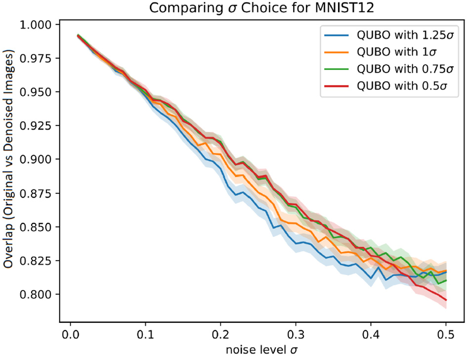
Figure 2. Proportion of pixels in denoised MNIST images that matched the original image, for different denoising methods with 95% CI error bars.

FIGURE 3

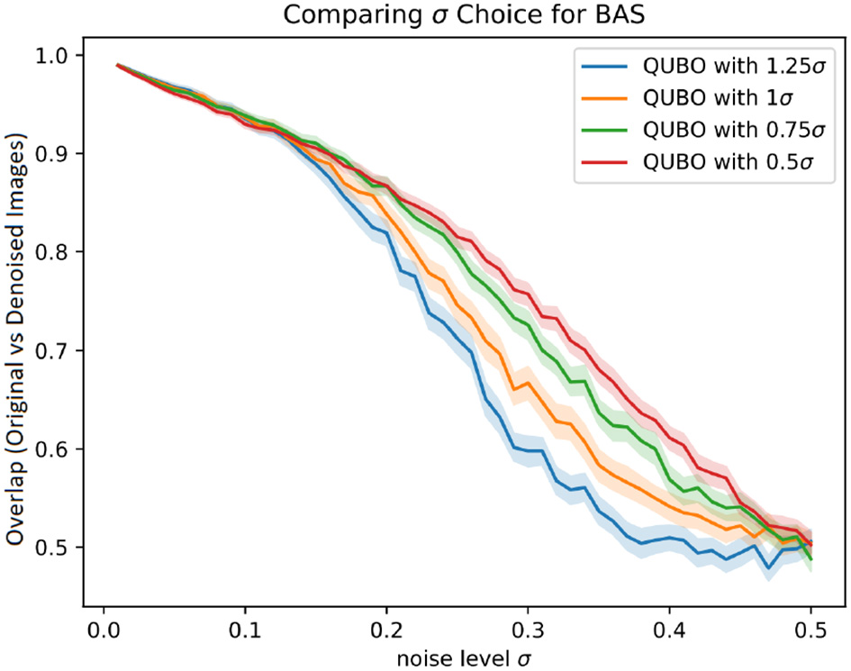
Figure 3. Proportion of pixels in denoised BAS images that matched the original image, for different denoising methods with 95% CI error bars.

Based on the empirical performance, using a bias factor of around 0.75 seems to give an improved performance compared to using a bias factor of 1 in both data sets. A bias factor of 0.5 seems to perform quite well-across most noise regimes as well, with largely overlapping confidence regions to the 0.75 parameter setting, though in the low-noise setting for the BAS dataset we observe an adverse effect. The authors thus suggest a setting of 0.75 for the bias factor.

Next, in Figures 4, 5, we compare our method to popular other denoising methods for binary images on the 12 × 12 MNIST and bars-and-stripes datasets, respectively, across different noise levels. When comparing to other methods, a crucial factor is that we choose ρ based off of σ, but in practice σ may be unknown. In light of this, we include two versions of our method in these comparisons. First, we use our method with $\rho :=log\frac{1-\sigma }{\sigma }$, using the true value of σ without introducing the recommended bias factor. Secondly, we simulate the situation in which the true σ is unknown, and instead we only have a guess for σ. To simulate having an approximate guess for σ, for each image afflicted by noise of level σ, we sample σ′ uniformly from an interval of size σ/2 centered at sigma. We then set $\rho :=log\frac{1-0.75{\sigma }^{\prime }}{0.75{\sigma }^{\prime }}$, using a bias factor of 0.75 on with this “guessed” value of σ. This is a significantly more realistic way of testing our method, since it gives an idea of how well the method may perform when the true noise level present in the noisy images is unknown and must be guessed. Our implementation here only assumes that the practitioner roughly knows the magnitude of the noise. For example, if the true noise is σ = 0.2, here we sample σ′ uniformly from [0.15, 0.25] to simulate the guess.

FIGURE 4

Figure 4. Proportion of pixels in denoised MNIST images that matched the original image, for different denoising methods with 95% CI error bars.

FIGURE 5

Figure 5. Proportion of pixels in denoised BAS images that matched the original image, for different denoising methods with 95% CI error bars.

We compare our method to Gibbs denoising with an RBM (Tang et al., 2012, Section 3.2), median filtering (Huang et al., 1979), Gaussian filtering (Stockman and Shapiro, 2001, Chapter 5), and a graph-cut method (Greig et al., 1989) for denoising. For the Gibbs denoising, we use the same well-trained RBM as for our QUBO-based method, and parameters of the method were carefully tuned for best performance to use 20 Gibbs iterations to then construct the denoised image as the exponentially weighted average of the samples with decay factor 0.8. Notably, as Gibbs-based denoising also requires a well-trained RBM, this method incurs the same computational overhead of training an RBM as our method does. However, it has the disadvantage of requiring careful tuning of the hyperparameters of the number of Gibbs iterations and decay factor to use, whereas our method of picking ρ is much more straightforward and shows good results without tuning. For the graph-cut method, the recommended parameter setting in the reference of β = 0.5 is used. The median filter, Gaussian filter, and Gibbs denoising (excluding the overhead of training the RBM) each have complexity O(n), where n is the number of pixels, whereas the graph-cut method has complexity O(n³) since a maximum-flow problem is solved on a graph whose nodes are the pixels of the image. Keeping the annealing time and number of reads as constant, the scaling of our method is also O(n). We forego wall-time here, since the software implementations we compare against are specialized for large problems, so comparing walltime for the small problems that can be implemented on current quantum annealers may not be representative. However, we note that for the QUBO denoising as we use up to 50μs annealing time and 100 reads per image, denoising an image only takes a total of 5ms of annealing time in our case.

Results are summarized in Figures 4, 5. Overall, the QUBO-based method performs quite strongly. Across all noise regimes in the MNIST data, and in most noise regimes in the bars-and-stripes dataset, the method outperforms the others. In particular, for the MNIST data the 95% confidence region for the QUBO method entirely dominates the others. Indeed, we see the good performance that our analysis from Section 3 suggests, even when the true σ is unknown and instead guessed. Using a guessed σ and the robustness modification of Section 3.3 makes the method perform as well (if not slightly better) as knowing the true σ without the robustness modification. Only in the noise regime of σ ≥ 0.2 in the BAS data does Gibbs denoising outperform our method.

4.3. Testing on larger images

Though we see the the straightforward implementability of our method on quantum annealers as a strong positive, a current drawback on using QAs is the limited data size that can be handled to accomodate their still small qubit capacities. Of course we can still instead test our method on larger datasets by obtaining solutions to the denoising QUBO 6 using other means. In Figure 6, we implement our method on a binarized version of the popular MNIST dataset (LeCun et al., 2010) by using simulated annealing (Kirkpatrick et al., 1983) to find solutions to (6). We particularly choose to test on the full-size MNIST dataset since we could only use a downscaled version on the QA due to size limitations on the input data, so this experiment serves to test our method without this downscaling. All methods are implemented as described in Section 4.1, and again for our method we use a guessed σ to simulate the unknown σ case and bias the guess for robustness.

FIGURE 6

Figure 6. Proportion of pixels in denoised images that were correctly denoised, for different denoising methods on the MNIST dataset, with 95% confidence intervals shaded.

5. Conclusion and future work

We investigated an image denoising framework via a penalty-based QUBO denoising objective that shows promise both theoretically through its statistical properties and practically through its empirical performance together with the proposed robustness modification. The method is well-suited for implementability on a quantum annealer, providing an important application of QAs within machine learning through the fundamental image denoising task. Good results are still obtained on larger datasets when the QUBO is only classically approximated by simulated annealing instead, revealing the approach to be promising even in the absence of QAs. As RBMs form a core building block of many deep generative models such as deep Boltzmann machines or deep belief networks (Goodfellow et al., 2016), a natural next step is to attempt to incorporate this approach into these more complex models, though current hardware limitations on existing quantum annealers are restrictive. Further, since our method takes advantage of QAs for the denoising step, further research into making use of QAs for the training process of RBMs would yield a full image denoising model where both the model training and image denoising make use of QA.

Data availability statement

The datasets presented in this study can be found in online repositories. The names of the repository/repositories and accession number(s) can be found below: https://github.com/PhillipKerger/Code_for_figures_of_QUBO_RBM_denoising_paper.

Author contributions

PK: Conceptualization, Formal analysis, Investigation, Methodology, Project administration, Software, Validation, Visualization, Writing—original draft, Writing—review and editing. RM: Conceptualization, Formal analysis, Funding acquisition, Project administration, Resources, Software, Supervision, Writing—review and editing.

Funding

The author(s) declare financial support was received for the research, authorship, and/or publication of this article. PK was supported in part by g-RIPS Sendai, Cyberscience Center at Tohoku Univ., and NEC Japan, in early stages of the work. PK is grateful to the USRA Feynman Academy internship program, support from the NASA Academic Mission Services (contract NNA16BD14C), and funding from DARPA under DARPA-NASA agreement SAA2-403688.

Acknowledgments

The early stage of this work is based on the work in the g-RIPS Sendai 2021 program. The authors thank Y. Araki, E. Escobar, T. Mihara, V. Q. H. Huynh, H. Kodani, A. T. Lin, M. Shirane, Y. Susa, and H. Suito for collaboration in the program. The authors also acknowledge H. Kobayashi and M. Sato for the use of the computing environment in the program. PK thanks Y. Sukurdeep for helpful feedback and discussions.

Conflict of interest

RM was employed by NEC Corporation.

The remaining author declares that the research was conducted in the absence of any commercial or financial relationships that could be construed as a potential conflict of interest.

Publisher's note

All claims expressed in this article are solely those of the authors and do not necessarily represent those of their affiliated organizations, or those of the publisher, the editors and the reviewers. Any product that may be evaluated in this article, or claim that may be made by its manufacturer, is not guaranteed or endorsed by the publisher.

Footnotes

1. ^https://github.com/PhillipKerger

References

Adachi, S. H., and Henderson, M. P. (2015). Application of quantum annealing to training of deep neural networks. ArXiv. ArXiv:1510.06356. doi: 10.48550/arXiv.1510.06356

CrossRef Full Text | Google Scholar

Albash, T., and Lidar, D. A. (2018). Adiabatic quantum computing. Rev. Mod. Phys. 90, 15002. doi: 10.1103/RevModPhys.90.015002

CrossRef Full Text | Google Scholar

Barahona, F. (1982). On the computational complexity of Ising spin glass models. J. Phys. A Math. Gen. 15, 3241–3253. doi: 10.1088/0305-4470/15/10/028

CrossRef Full Text | Google Scholar

Benedetti, M., Realpe-G'omez, J., Biswas, R., and Perdomo-Ortiz, A. (2015). Estimation of effective temperatures in quantum annealers for sampling applications: a case study with possible applications in deep learning. Phys. Rev. A 94, 022308. doi: 10.1103/PhysRevA.94.022308

CrossRef Full Text | Google Scholar

Boyat, A. K., and Joshi, B. K. (2015). A review paper: noise models in digital image processing. ArXiv. doi: 10.5121/sipij.2015.6206

CrossRef Full Text | Google Scholar

Buades, A., Coll, B., and Morel, J.-M. (2005). A review of image denoising algorithms, with a new one. Multiscale Model. Simul. 4, 490–530. doi: 10.1137/040616024

CrossRef Full Text | Google Scholar

Cho, K. (2013). Boltzmann machines and denoising autoencoders for image denoising. ArXiv. ArXiv:1301.3468. doi: 10.48550/arXiv.1301.3468

CrossRef Full Text | Google Scholar

Das, A., and Chakrabarti, B. K. (2008). Colloquium: quantum annealing and analog quantum computation. Rev. Mod. Phys. 80, 1061–1081. doi: 10.1103/RevModPhys.80.1061

CrossRef Full Text | Google Scholar

Dixit, V., Selvarajan, R., Alam, M. A., Humble, T. S., and Kais, S. (2021). Training restricted boltzmann machines with a d-wave quantum annealer. Front. Phys. 9, 589626. doi: 10.3389/fphy.2021.589626

CrossRef Full Text | Google Scholar

Glover, F. W., Kochenberger, G. A., and Du, Y. (2018). Quantum bridge analytics i: a tutorial on formulating and using qubo models. 4OR 17, 335–371. doi: 10.1007/s10288-019-00424-y

CrossRef Full Text | Google Scholar

Goodfellow, I. J., Bengio, Y., and Courville, A. (2016). Deep Learning. Cambridge, MA: MIT Press. Available online at: http://www.deeplearningbook.org (accessed August 20, 2023).

Google Scholar

Greig, D., Porteous, B., and Seheult, A. H. (1989). Exact maximum a posteriori estimation for binary images. J. R. Stat. Soc. Ser. B Methodol. 51, 271–279. doi: 10.1111/j.2517-6161.1989.tb01764.x

CrossRef Full Text | Google Scholar

Hinton, G. E. (2002). Training products of experts by minimizing contrastive divergence. Neural Comput. 14, 1771–1800. doi: 10.1162/089976602760128018

PubMed Abstract | CrossRef Full Text | Google Scholar

Huang, T. S., Yang, G., and Tang, G. (1979). A fast two-dimensional median filtering algorithm. IEEE Transact. Acoust. Speech Signal Process. 27, 13–18. doi: 10.1109/TASSP.1979.1163188

CrossRef Full Text | Google Scholar

Johnson, M. W., Amin, M. H. S., Gildert, S., Lanting, T., Hamze, F., Dickson, N., et al. (2011). Quantum annealing with manufactured spins. Nature 473, 194–198. doi: 10.1038/nature10012

PubMed Abstract | CrossRef Full Text | Google Scholar

Kadowaki, T., and Nishimori, H. (1998). Quantum annealing in the transverse ising model. Phys. Rev. E 58, 5355–5363. doi: 10.1103/PhysRevE.58.5355

CrossRef Full Text | Google Scholar

Kirkpatrick, S., Gelatt, C. D., and Vecchi, M. P. (1983). Optimization by simulated annealing. Science 220, 671–680. doi: 10.1126/science.220.4598.671

CrossRef Full Text | Google Scholar

Koshka, Y., and Novotny, M. A. (2021). Comparison of use of a 2000 qubit d-wave quantum annealer and mcmc for sampling, image reconstruction, and classification. IEEE Transact. Emerg. Top. Comp. Intell. 5, 119–129. doi: 10.1109/TETCI.2018.2871466

CrossRef Full Text | Google Scholar

Krzysztof, K., Mateusz, S., Marek, S., and Rafał, R. (2021). Applying a quantum annealing based restricted boltzmann machine for mnist handwritten digit classification. Comp. Methods Sci. Technol. 27, 99–107. doi: 10.12921/cmst.2021.0000011

CrossRef Full Text | Google Scholar

LeCun, Y., Cortes, C., and Burges, C. (2010). Mnist Handwritten Digit Database. ATT Labs. Available online at: http://yann.lecun.com/exdb/mnist (accessed August 20, 2023).

Google Scholar

Lucas, A. (2014). Ising formulations of many NP problems. Front. Phys. 2, 5. doi: 10.3389/fphy.2014.00005

CrossRef Full Text | Google Scholar

Nishimori, H. (2001). Statistical Physics of Spin Glasses and Information Processing: An Introduction. New York, NY: Oxford University Press.

Google Scholar

Rudin, L. I., Osher, S., and Fatemi, E. (1992). Nonlinear total variation based noise removal algorithms. Phys. D 60, 259–268. doi: 10.1016/0167-2789(92)90242-F

CrossRef Full Text | Google Scholar

Stockman, G., and Shapiro, L. G. (2001). Computer Vision. Upper Saddle River, NJ: Prentice Hall PTR.

Google Scholar

Tang, Y., Salakhutdinov, R., and Hinton, G. E. (2012). “Robust boltzmann machines for recognition and denoising,” in 2012 IEEE Conference on Computer Vision and Pattern Recognition (Providence, RI), 2264–2271.

Google Scholar

Vahdat, A. (2017). “Toward robustness against label noise in training deep discriminative neural networks,” in NeurIPS Proceedings 2017 (Long Beach, CA).

Google Scholar