Interactive landscape–scale cloud animation using DCGAN

1. Introduction

Cloud animation at real-time or interactive frame rates is a challenging task in computer graphics (CG). Procedural methods are capable of producing high-quality static clouds in movies. However, in order to animate the clouds, a physics-based simulation (Eulerian or Lagrangian) operating at a reasonably high resolution is required. In most cases, these simulations are computationally and memory-wise too intensive for any real-time considerations (Goswami, 2020). Furthermore, almost oblivious to the simulation method applied, a rendering pass is needed to visualize the simulated cloud data. This makes the overall process not only quite time-consuming (even on a GPU) but also dependent on various factors that necessitate human intervention to define and adjust variables throughout the simulation process.

Modern CG and multimedia applications are increasingly benefiting from using artificial intelligence (AI) algorithms (Agrawal, 2018). This incorporation or blend has several advantages. For example, it can automate several tasks and even computationally accelerate the underlying model by learning and predicting from the data. In addition, the enormous amount of available data that can be processed and used for training and the growing hardware processing power add to the successful integration of AI and CG-based approaches.

In this study, we introduce machine learning in the context of synthesizing landscape-scale cloud animations. When trained on real-life cloud videos, the machine learning model is leveraged to produce natural-looking cloud animations. To this end, we use deep convolutional generative adversarial network (DCGAN), which is an unsupervised learning algorithm. Contrary to several applications that have successfully employed DCGAN to generate images, we demonstrate the potential of generating animations using a variant of DCGAN.

The main contributions of our approach are as follows:

• An efficient way of producing automatic, landscape-scale 3D cloud animation at interactive frame rates with the help of a state-of-the-art machine learning algorithm (i.e., DCGAN).

• A rich animation pattern inspired by real-life clouds by employing DCGAN on the GPU for training and generating coherent, sequential images.

• A high-resolution 3D animation produced from small-sized image patches generated by a deep learning model.

• A new interpolation-based algorithm to generate new artificial image sequences using the constructed DCGAN model.

• A preprocessing method that can easily rely on home-captured videos for training to achieve high-quality results.

The proposed approach handles cloud evolution through DCGAN, thereby eliminating the use of any underlying cloud physics. We, therefore, save computations and memory by avoiding the expensive physics-based models that are otherwise employed to generate these animations, albeit at a low resolution and for a limited volume of cloud. Nevertheless, the user retains the ability to modify some parameters, such as cloud coverage level in the sky, without needing to alter training data sets. This gives us the advantage that our method can easily be used for background cloud generation while preserving a higher computational bandwidth for the primary task. This advantage is essential as most applications containing clouds require that they cover a detailed expanse of the sky and only take a fraction of the computational frame time. This contradictory requirement is a huge challenge for traditional physics-based simulation methods, which we circumvent with the proposed method.

We simplify preprocessing by limiting the size of input training images given to the neural network while still obtaining high-resolution animation sequences. Though we demonstrate our technique for cumulus clouds, it could easily be generalized to other cloud types by altering the training data sets and possibly the renderer. Finally, we adopt the human-visual system scoring to help compare the visual quality of our obtained cloud animations. We have conducted a participant evaluation of 41 participants, most of whom voted in favor of our proposed machine learning-based method compared with an existing physics-based approach.

It is important to stress that our contribution is independent of Generative Adversarial Network (GAN) architectures. Our preprocessing approach to generate animations can be plugged into any type of GANs. Following this, it basically boils down to the training process and the algorithm generating the animation sequences of clouds. However, we discuss and justify our choice of DCGAN for the proposed approach (see Section 3.2.1).

2. Related work

Clouds in CG and multimedia have been studied from various angles, including modeling, rendering, and animation. Here, we will keep our discussion focused on the animation methods, which is the aspect most related to ours. Up until recently, most of the developed cloud animation methods were offline. Clouds have been animated with the help of both procedural and physics-based approaches. Recently, some physics-based methods have been developed that can support real-time or interactive frame rates on GPU. One limitation of most of these methods is that they are forced to simulate a limited volume of the sky, often at a low resolution, due to the sheer magnitude of computations and usage of memory involved. We refer the reader to Goswami (2020) for an in-depth survey on cloud modeling, rendering, and animation.

Related literature is grouped into different categories to ease visualizing prior works.

2.1. Procedural methods

Procedural techniques have been proposed to produce the effect of evolving clouds, wherein the illusion of animation is produced without using any actual physics. In the method by Dobashi et al. (1998) and Bi et al. (2016), simple transition rules on cellular automata have been demonstrated to produce offline clouds. Jhou and Cheng (2016) animated still landscape photographs by animating the cloud cover present in them. The animation produced, however, is limited due to the limited variation between frames. Webanck et al. (2018) achieve cloud modeling and animation clouds with a purely procedural, offline approach that uses field functions to generate different cloud types. Logacheva et al. (2020) generate realistic time-lapse landscape videos with moving objects and other time-of-the-day changes with the help of a StyleGAN-based model.

2.2. Physics-based methods

Most of the earlier cloud simulation work has focused on Eulerian solvers coupled with simplified cloud dynamics. Schpok et al. (2003) animated clouds using a two-level approach, wherein larger movements are governed by the macro-level and smaller changes are a function of the micro-level animation. Harris et al. (2003) animated small changes in the cloud structure handled with the help of GPU-sliced textures. Later, work also explored the particle-based approach for cloud animation. Neyret (1997) applied high-level physics-based variables to obtain an approximate, perceptually convincing simulation of convective clouds. A particle-based cloud simulation on GPU is presented by Barbosa et al. (2015). The simulation is adaptive and relies on position-based fluid dynamics and cloud physics to achieve simulation in a small domain. A target-driven cloud evolution method using position-based fluids on particles is developed by Zhang et al. (2020a).

2.3. Hybrid methods

More recently, the idea of hybrid physics-based procedural animation is introduced by Goswami and Neyret (2017). The physics component, which constitutes a higher computational cost, is carried out at the macro level, and procedural hypertexture amplification is carried out at the micro level based on the underlying physics parameters. This idea is further improved by Goswami (2019), wherein a cloud map is introduced to eliminate volumetric amplification inside the spherical parcels. The obtained benefits are more realistic cloud shapes at higher frame rates. However, the animation pattern of such generated clouds is not entirely realistic. Hädrich et al. (2020) have recently simulated a variety of clouds using a set of lightweight higher level primitives. Vimont et al. (2020) have employed a similar concept in Eulerian settings instead of the Lagrangian framework. Duarte and Gomes (2017) simulated air parcels in real time by using the sounding data from dataSkewT/LogP diagrams.

The research gap to utilize AI algorithms to the end of cloud animation is clearly outlined by Goswami (2020). Machine learning has been used to automate cloud illumination (Kallweit et al., 2017). In their method, radiance predicting neural network obtains illumination hints from the lighted cloud images. Similarly, 3D cloud shapes are modeled, taking inspiration from real-life cloud shapes present in the images (Yuan et al., 2014). To the best of our knowledge, no work, with the exception of Zhang et al. (2020b), has adopted this approach for animating clouds. Zhang et al. apply a combination of convolutional neural networks and computational fluid dynamics to generate clouds with the desired shapes. However, their method does not work in real time and is shown to generate a limited volume of clouds.

The proposed work bridges the aforementioned research gap by introducing a DCGAN-based machine learning method that produces rich and realistic 3D cloud animations at interactive frame rates for landscape-scale terrain cloud coverage. Unlike most previous works, our method supports cloud visualization and its time-based evolution for the scale of the entire visible landscape and not just for a small, limited sky volume.

3. Methodology

Our method aims to generate realistic cloud animations for a given landscape-scale sky by learning cloud evolution from simple videos containing this information. Our definition of the landscape-scale is consistent with that reported by Lee and Huh (2020). Even though our technique learns the animation from small-sized image frames, it is capable of producing a much higher resolution 3D cloud animation with the help of learned image animation sequences. Figure 1 shows the overview of our approach. The input to our method is the user-captured videos containing clear, gradual cloud evolution over a period of time during the day. Given an initial input cloud image sequence, the output consists of a sequence of coherent animation frames of the same size, as the input image obtained with the help of our proposed pipeline. To make the whole process efficient, we limit ourselves to videos and images with small dimensions. This reduces the preprocessing and machine learning overhead drastically. In addition, the chosen frame size does not seem to pose any restriction on the quality of generated cloud animation. The frame size, however, turns out to be a limiting factor for the output visualization. We circumvent this by using the output animation as a cloud map in an existing 3D application. First, this helps us to animate a 3D cloud cover (using output cloud images) over a much larger landscape than the image dimensions on which the neural network is operating. Second, it enables us to customize and create a 3D background of our choice that can house animated clouds from our method independently.

FIGURE 1

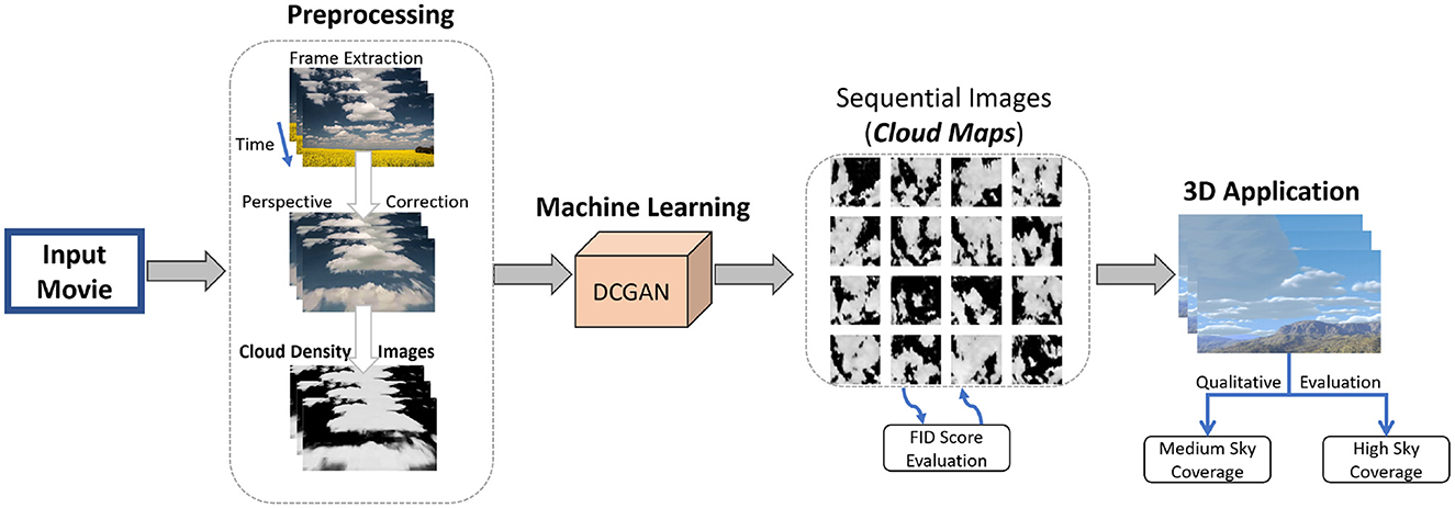
Figure 1. Overview of our method. In the preprocessing stage, input video frames are extracted and cropped for regions containing cloud animation. Subsequently, we applied other corrections to produce density cloud images, which are given as input to the DCGAN for learning. The output of DCGAN is the sequential cloud images, which are plugged into a 3D rendering application.

We first introduce various preprocessing steps performed on the source videos in the following Section 3.1. These steps are essential to obtain a coherent and efficient training image sequence that can be a clean input to the DCGAN algorithm. After extracting frames from each source video, we crop the images to isolate the area containing clouds and subject them to a perspective correction phase. Furthermore, the processed frame's intensity dynamic range is then normalized, leading to the background and foreground separation, and subsequently adjusted for factors such as contrast, making the learning more robust while minimizing the influence of irrelevant factors. In Section 3.2, the DCGAN-based machine learning model is explained in detail, which is the next step after obtaining the preprocessed frames.

3.1. Data set: Video source and preprocessing

A total of 13 video files of real-life cumulus clouds recorded from ground level were collected, nine of which were obtained from publicly available data sets (Setvak, 2003; Jacobs et al., 2013; 2016), and the authors captured four videos. All but one of the 13 source videos contained both sky and landscape. Each video from the publicly available data sets contained brief details at the beginning of the video (information about the photographer, the location, and the camera lens used) (Setvak, 2003). Hereafter, we refer to this total collection of videos as the cloud data set.

The source videos are clipped to include a continuous and consistent sequence of cloud frames without any overlay text or sudden jump to different time points. The frames of the source videos, denoted as λ_source, are then cropped to exclude any landscape λ_cropped visible in the video (see also Figure 2). For our purpose, we captured videos with a static camera, which simplified the cropping process. In the following, we explain the sequential preprocessing steps, which are required to produce the necessary cloud-density images. These cloud-density images are supplied as input for the deep learning model.

FIGURE 2

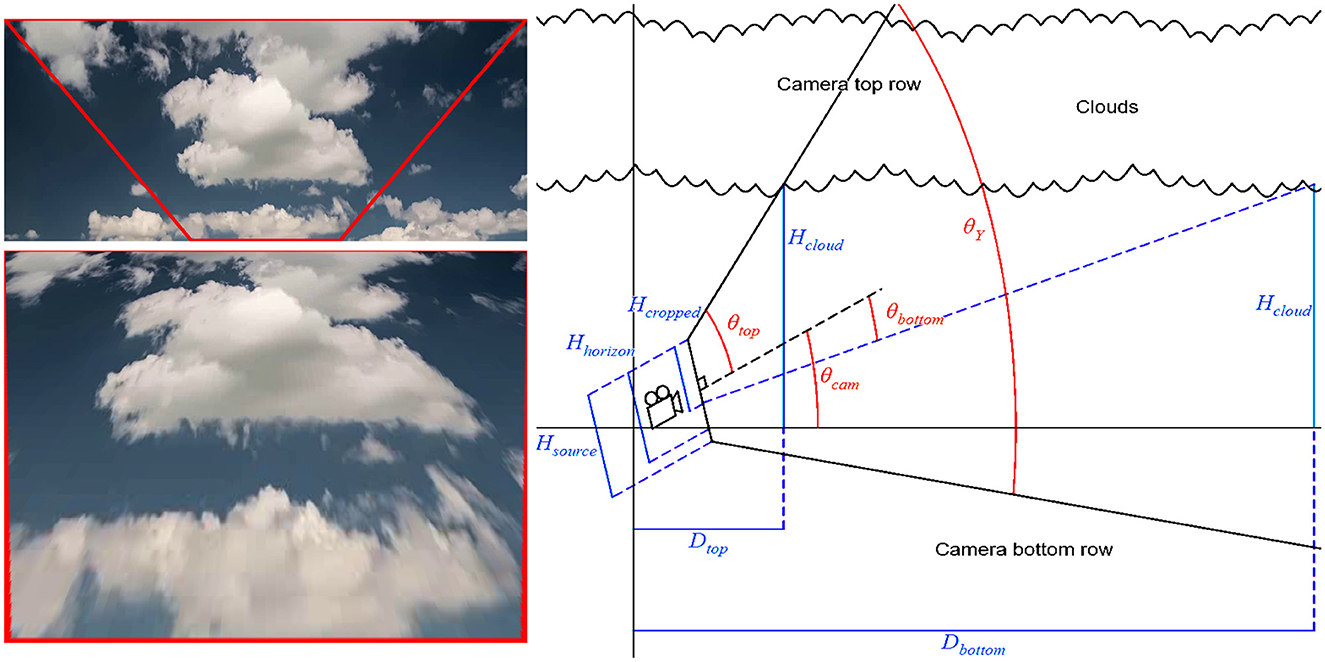
Figure 2. λ_cropped with its four points forming the corners of a convex isosceles trapezium (top left). λ_cropped after perspective correction into λ_corrected (bottom left). Note how the bottom corners of the trapezium have been stretched to the bottom corners. Side-view visual representation of the calculations of Equations (1)–(3), which later leads to determining the final two points in λ_cropped (right).

3.1.1. Perspective correction

Images or videos captured using any camera contain different levels of perspective distortions. To generate a good training data set over images, it is essential to correct this distortion as much as possible. This is especially true in our case since we employ 2D cloud images containing no perspective distortion (akin to a cloud map), to generate a 3D cloud cover. The corrected image, denoted as λ_corrected, is obtained by applying a 3 × 3 transformation matrix to λ_cropped. This matrix is calculated by using the projective method for solving the homography decomposition problem described theoretically by Malis and Vargas (2007) and Szeliski (2010) and implemented in OpenCV using the findHomography function (2020a). Four points in λ_cropped and their corresponding points in λ_corrected are required for the function to determine the transformation and calculate the matrix (Figure 2). Two of the image's four points in λ_cropped are located in the top left and top right corners. The other two are located along with the bottom row, equal distances from the left and right edges. Their four corresponding points in λ_corrected are all located at the corners of the image. As six of the eight total points were predetermined at the corners of the images, only the two bottom points in λ_cropped are needed to be calculated. Being located at the bottom row of λ_cropped meant that only their horizontal positions are required, which is performed according to the following sequential steps. H_cloud in the following section is a pixel estimate of the height at the bottom of the cloud, estimated by using elevation values for cumulus clouds in the given frame.

• Determine the vertical and horizontal fields of view of the camera lens; this is done by finding the specification of the lens used and hence its focal length range. This step provides us with vertical (θ_Y) and horizontal (θ_X) fields of view.

• Determine the pixel height of the horizon line in λ_source. The row closest to the horizon line determines its pixel height, denoted as H_horizon, and H_source is the pixel height of the source image λ_source.

• Calculate the vertical angle between the ground and the direction the camera is aiming (θ_cam) at as follows:

$\begin{array}{ll}{\theta }_{cam}=(\frac{H_{horizon}}{H_{source}}-\frac{1}{2}){\theta }_Y,& (1)\end{array}$

where θ_cam > 0 if $H_{horizon}>\frac{H_{source}}{2}$.

• Calculate the vertical angle between the top of clouds and the middle of λ_source. As the top of λ_source has no landscape, the angle between the center of λ_source and the top part of clouds on λ_source, denoted as θ_top, is equal to $\frac{{\theta }_Y}{2}$. The angle between the center of λ_source and the bottom of λ_cropped, denoted as θ_bottom, is calculated as follows:

$\begin{array}{ll}{\theta }_{bottom}=(\frac{1}{2}-\frac{H_{cropped}}{H_{source}}){\theta }_Y,& (2)\end{array}$

where H_cropped is the pixel height of λ_cropped.

• Calculate the vertical angle between the bottom of the clouds and the middle of λ_source.

• Calculate the depth of clouds in the image at the top and bottom of λ_cropped. The horizontal depths of the clouds at the top and bottom of λ_cropped, denoted as D_top and D_bottom, respectively, are calculated as follows:

$\begin{array}{ll}{D}_{top/bottom}=\frac{H_{cloud}}{tan({\theta }_{cam}+{\theta }_{top/bottom})}& (3)\end{array}$

Here, θ_cam+θ_top and θ_cam+θ_bottom are the angles between the ground and directions to the top and bottom of the clouds in λ_cropped.

• Calculate the width of clouds, along the edges, at the top and bottom of λ_cropped. Using the horizontal field of view, the widths of clouds at the top and bottom of λ_cropped, denoted as W_top and W_bottom, are calculated as follows:

$\begin{array}{ll}{W}_{top/bottom}=2D_{top/bottom}tan(\frac{{\theta }_X}{2})& (4)\end{array}$

W_top and W_bottom now represent an approximate distance between the clouds, seen at the top and bottom of λ_cropped, along its left and right edges.

• Let us calculate the ratio between the widths at the top and bottom ($R=\frac{W_{bottom}}{W_{top}}$) of λ_cropped. The formula for R is rewritten and simplified by combining Equations (1)–(4) as follows:

$\begin{array}{ll}R=\frac{tan(\frac{H_{horizon}}{H_{source}}{\theta }_Y)}{tan(\frac{H_{horizon}-H_{cloud}}{H_{source}}{\theta }_Y)}.& (5)\end{array}$

• Calculate the two bottom points in λ_cropped. Finally, the horizontal positions X_left and X_right of the bottom points in λ_cropped are calculated as follows:

$\begin{array}{ll}{X}_{left/right}=\frac{W_{cropped}}{2}(1\mp \frac{1}{R}),& (6)\end{array}$

where W_cropped is the pixel width of λ_cropped.

After passing the two sets of four points to findHomography, the returned matrix is used with OpenCV's warpPerspective on every image λ_cropped to generate its respective λ_corrected.

3.1.2. Grayscale conversion

In the cropped and perspective-corrected sky images, we need to automate the separation of foreground cloud pixels from the sky background. To this end, we first convert the color channels of λ_corrected to a grayscale image, clamping the values to a certain threshold and brightening as well as blurring the image using the normalized B/R ratio function proposed by Li et al. (2011).

$\begin{array}{ll}{\lambda }_N=\frac{b-r}{b+r},& (7)\end{array}$

where r and b represent the values of the red and blue channels of the original image. Thus, λ_N becomes a flattened image with a single channel, where each pixel is a rational value between −1 and 1. Pixel values of λ_N, in this case, are found to be close to −1 if their probability to belong to cloud regions is high and close to 1. In this step, subtraction in the numerator is flipped as the pixels of a cloud need to be represented by high values. This mapped image is, then, re-scaled to an interval between 0 and 1 and multiplied by 255 to yield an 8-bit unsigned matrix.

$\begin{array}{ll}{\lambda }_N=\frac{{\lambda }_N+1}{2}\times 255,& (8)\end{array}$

resulting in the combined formula as follows:

$\begin{array}{ll}{\lambda }_N=\frac{\frac{r-b}{r+b}+1}{2}\times 255.& (9)\end{array}$

The matrix λ, thus, results in an image where the sky has varying shades of dark gray and the clouds are in light gray.

3.1.3. Contrast adjustment

As λ_N contains the sky which is not uniformly black and clouds not uniformly white, the contrast of pixels needs to be corrected for easy discernment. Before normalizing the pixels of the cloud map λ_N to values between 0 and 1, a threshold (T) is defined. All pixels with values below T are to be considered as the sky with no cloud. Pixel values are clamped to a range between T and 1,

$\begin{array}{ll}{\lambda }_T=\text{min}(\text{max}({\lambda }_N,T),1),& (10)\end{array}$

where −1 ≤ T < 1. If the pixel values were to be normalized at this stage using Equation (8), the lowest value of the resulting range would be $\frac{T+1}{2}$ rather than 0. Instead, the following equation is used to normalize λ_T to values between 0 and 1.

$\begin{array}{ll}{\lambda }_{TN}=\frac{{\lambda }_T-T}{1-T}& (11)\end{array}$

T is determined empirically by applying the cloud map steps on a data set comprising different source video files collected locally (i.e., 13 video files constituting our cloud data set). The lowest value of T = −0.25 was chosen, which caused the entire background sky to become black in most of these videos (i.e., the sky in λ_TN is uniformly black). However, the cloud regions still needed some brightness enhancements. The brightness-enhancing function we used is a version of the SmoothStop (SS) function introduced by Squirrel (Eiserloh, 2015), which is as follows:

$\begin{array}{ll}\text{SS}(t)=1-{(1-t)}^8,& (12)\end{array}$

This was applied at the pixel level of the cloud map. The exponent 8 was chosen, as it is the lowest integer causing the brightest pixels to saturate. After brightening the cloud maps with SS, they are passed through a 5 × 5 Gaussian blur filter to reduce any potential noise introduced in the perspective correction step. This is the final preprocessing step before cloud maps are used to train the machine learning model.

It is worth noting that when constructing an algorithm to separate clouds from the sky of ground-level footage, several approaches have been suggested using a ratio or a difference between the color channels of each pixel in the image. Heinle et al. (2010) used the differences R−B between red and blue channels to convert a colored image to a grayscale image, followed by thresholding to distinguish cloud and sky regions. Kazantzidis et al. (2012) used a multicolor criterion B < R+20 & B < G+20 & B < 60, taking into account the green channel as well. However, in our case, their method did not achieve the intended classification, as it identified cloud areas not containing the direct solar glare as sky regions. A Hybrid Thresholding Algorithm (HYTA) used to detect clouds was put forward by Li et al. (2011). They propose the normalized B/R ratio λ_N = (B−R)/(B+R) alongside an adaptive threshold rather than a fixed one for increased accuracy. This algorithm produced cloud maps with the most diverse colors between the clouds and the sky in our case.

3.2. Deep learning

In the context of deep learning, GANs employ an adversarial process to train and predict (Goodfellow et al., 2020). GAN is a family of training and prediction of deep learning algorithms that have proved to be an essential turning point in generative modeling (Park et al., 2021), especially while dealing with image-based data. GAN differs from other machine learning approaches in which training is conducted by two different networks: the generator and the discriminator. The generator model generates real-like data from an input (e.g., random noise), and the discriminator evaluates the generated data to decide whether it is natural or synthetic.

While the original GAN has shown promising results in generating images from features it learned from input images, the images it generated lacked quality and comprehensibility. Furthermore, GANs often require hundreds of hours of training time when tasked with, for example, learning the structure of faces (Karras et al., 2018, 2019a). Larger networks can not only generate images with higher fidelity but also require more hours of training time and more data. DCGAN (Radford et al., 2016) was developed to further improve upon GAN. DCGAN uses convolutional layers in the network and employs batch normalization in between these layers to stabilize the learning. Furthermore, dropout layers are added between each convolutional layer with some connections between layers, so the values of certain nodes are not fed-forward. The generator uses Rectifier Linear Unit (ReLU) as the activation function between the layers, which was shown to help the generator to cover the color space of the training distribution more quicker. We, therefore, preferred DCGAN over GAN for our purpose. The input and output images to the DCGAN in all our cases had 256 × 256 dimensions. The grayscale images obtained from a preprocessing step are used for the purpose of training and generating animation frames. The machine learning model takes an input and generates a vector of 65,536 (256 × 256 × 1) 32-bit floating point values, which are then converted into 8-bit unsigned integer values.

3.2.1. Choice of GAN Model Variant

As has been noticed in (2022), the GAN family is constantly growing, and at the time of writing this study, there are more than 500 variants of GAN. To select a suitable GAN architecture, we compared three of the most commonly used variants, namely, the DCGAN (Radford et al., 2016), the simplified model (SGAN) (Chavdarova and Fleuret, 2018), and the Wasserstein model (WGAN) (Arjovsky et al., 2017). At the model architecture level, GANs are challenging to compare. Goodfellow (the creator of GANs) stated that GANs lack an objective function, which makes it difficult to compare the performance of different models (Salimans et al., 2016). A similar observation was made by Borji regarding the existence of several measures and yet the lack of identification of a precise measure that best captures the strengths and limitations of models (Borji, 2019). Nevertheless, GAN models could be evaluated based on the quality of the images they generate, often by using non-reference image quality metrics.

Our choice of using DCGAN is motivated by two important factors. First, NVIDIA has integrated DCGAN into their GPU library based on their successful experiments on images. Second, in order to further reinforce our choice of GAN architecture, we studied its relative performance with some of its competitors in our animation settings (SGAN and WGAN, as mentioned earlier). To this end, we adopted state-of-the-art quality metrics, namely, the blind/referenceless image spatial quality evaluator (BRISQUE) (Mittal et al., 2012) and the perception-based image quality evaluator (PIQE) (Venkatanath et al., 2015). As shown in Figure 3 and Table 1, the choice of DCGAN is justified for this study since its image output quality is proven to be better than those generated by SGAN and the WGAN. In addition, DCGAN has the least computational cost (on average per epoch, DCGAN is faster than SGAN and WGAN by 1.41- and 4.6-folds, respectively). As stated earlier, the proposed cloud animation approach is generic in that it can be implemented with any other suitable GAN architecture.

FIGURE 3

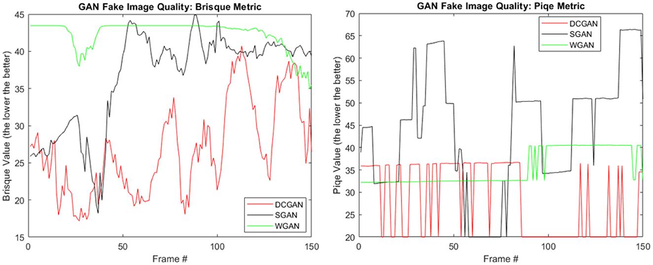
Figure 3. Image output quality assessment of different GAN models trained on 40K cloud images with similar settings. (Left) Quality assessment using BRISQUE and (right) PIQE.

TABLE 1

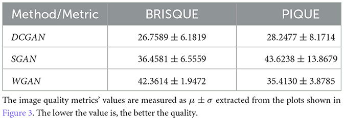
Table 1. Comparison of different GAN architectures.

3.2.2. Choice of DCGAN architecture

We considered and tested two different versions of DCGAN, one from the TensorFlow (2020b) and the other from Radford et al. (2016), hereafter referred to as T_DCGAN and R_DCGAN, respectively. After an architectural base has been established based on the results obtained, it needs to undergo a few configuration iterations to improve the training performance. The video data available for training was limited, and the original DCGAN configuration was insufficient for our training. The two chosen versions were compared in terms of the quality of the images and the time required to train the model for that particular quality by comparing their Fréchet Inception Distance (FID) scores. The generated GIF (Graphics Interchange Format) files were evaluated regarding how natural the animations looked.

Fréchet Inception Distance (FID) was first introduced by Heusel et al. (2017) and is shown to be a more consistent method of evaluating different GAN architectures' performance (Karras et al., 2018, 2019b, 2020). FID works by combining the Fréchet distance to measure the difference between synthetic and real-world images with the Inception score to measure the “objectness” and “diversity” of a synthetic image (Salimans et al., 2016). When combined, they give an evaluation of images that bear a closer resemblance to the human evaluation system (Heusel et al., 2017). Given the two activation feature vectors (2,048 lengths each), for the actual data sample (X_r) and model generated sample (X_g) of the final layer of the pre-trained Inception network, the FID can then be seen as the Wasserstein distance (W) between the two multivariate normal distributions, ${N}({\mu }_r,{\Sigma }_r)$ and ${N}({\mu }_g,{\Sigma }_g)$.

$\begin{array}{ll}\begin{array}{l}FID=W({N}({\mu }_r,{\Sigma }_r),{N}({\mu }_g,{\Sigma }_g))\\ =\parallel {\mu }_r-{\mu }_g{\parallel }^2+Tr({\Sigma }_r+{\Sigma }_g-2{({\Sigma }_r{\Sigma }_g)}^{1/2})\end{array}& (13)\end{array}$

where Tr is the trace linear algebra operation, μ_r and μ_g are the feature-wise mean values of the natural and generated images, respectively, and Σ_r and Σ_g are the covariance matrices for the natural and generated feature vectors, respectively.

3.2.3. Training

The training part begins after the architectural configuration is selected. Several aspects need to be taken into account when training a machine learning model. This entails tuning the hyper-parameters of the model (Kuhn and Johnson, 2013), supplying sufficient data and testing the generated content manually or automatically (Radford et al., 2016; Karras et al., 2018). The hyper-parameters of the training process were tuned in order to improve training efficiency. The most prevalent parameter was the learning rate, which is set at 2 × 10⁻³, following the default setup of common deep learning architectures (e.g., StyleGAN 2). To obtain a higher efficiency for learning, this parameter was tuned several times, and each trial was trained for several epochs. The testing consisted of a visual inspection of the generated content to see if the model collapsed, in which case the learning rate was too high and needed to be lowered. When a collapse occurs (Figure 4), it generates identical or quasi-identical images over and over again, independent of the input given to the model.

FIGURE 4

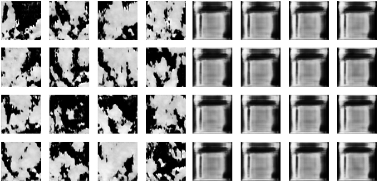
Figure 4. Images generated on cloud data set for training over 2,000 epochs with a learning rate of 5 × 10⁻⁵ using (left) TensorFlow (2020b) and (right) Radford et al. (2016) demonstrating a collapse of the model by generating identical images.

The learning rate was initially altered using the following equation L_n = L_n−1*0.1 where L_n is the current learning rate and L_n−1 is the previous learning rate. Once the model stopped collapsing early in the training process, the equation L_n = L_n−1*1.5 was used instead. By increasing the learning rate, the model can converge more quickly, which results in a shorter training time. Similar to a study by Meng et al. (2019), we have tried shuffling the input data to improve training performance and convergence in the setting of deep learning.

3.2.4. Generating animations

In a majority of the existing work on GAN and DCGAN, we found that the learning is employed to produce static images and not an animation sequence. However, a significant challenge in our work is to utilize DCGAN to generate a coherent sequence of smooth animation frames rather than a temporally uncorrelated sequence of frames. An important factor discovered during experimentation is that how input to the DCGAN is constructed plays a vital role in generating smooth and consistent animations. To this end, two different methods of generating the input values were tested.

The first method is presented in Algorithm 1 where F_r is a function that generates a random rational value between −1 and 1 each time it is called, a represents the absolute value of the highest possible value change, and V represents the input vector of the generator.

ALGORITHM 1

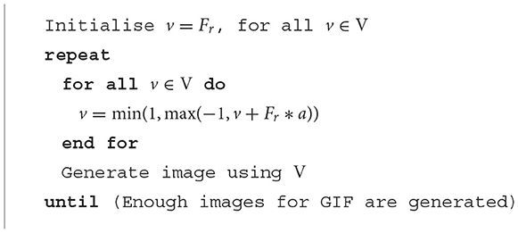
Algorithm 1. Updating the input vector - First method.

The main drawback we experienced with this method is its inability to transition over a large section of the input space smoothly. Instead, the values of the input vector transition back and forth within a confined space.

The second method of generating input vectors is presented in Algorithm 2. This method was chosen over the previous one, as it did not have the drawback of the first method and was able to generate consistent and smooth animations. A and B represent two vectors of the same dimensions as V, which are linearly interpolated between them. Here, t represents a value between 0 and 1 for the percentage of time that has passed between two time points, and n represents the dimension of the vectors. Δt is an incremental value defined in Equation (14) where Num is the number of cloud images we target to generate using DCGAN.

$\begin{array}{ll}\Delta t=\frac{1}{Num}& (14)\end{array}$

ALGORITHM 2

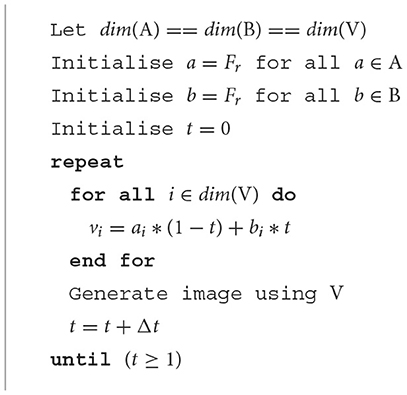
Algorithm 2. Updating the input vector - Second method.

The cloud map is updated by supplying the neural network with a 100-dimensional vector of pseudorandom rational values between −1 and 1. Over time, the cloud map is updated by generating two different 100-dimensional vectors and then linearly interpolating between them with the following equation:

$\begin{array}{ll}{v}_n=a_n*(1-t)+b_n*t& (15)\end{array}$

where v_n is the n:th value in the input vector V, a_n is the n:th value in vector A, b_n is the n:th value in vector B, and t is a rational value between 0 and 1. Such vectors are produced at set intervals on the CPU and passed on to the GPU to refresh the cloud map.

3.2.5. Application

As noted earlier, any neural network takes much longer to train on and produce large images. We have, therefore, restricted ourselves to an image dimension of 256 × 256 obtained after preprocessing (see Section 3.1), which is a good trade-off between size and training time. However, this size is still too small to produce a video with reasonably large frame dimensions. We have addressed this shortcoming by treating the trained and output image samples as cloud maps to be an input for our interactive animation method (Goswami, 2019). In the latter reference, a single 2D cloud map is mapped to the 3D world, and 3D clouds are obtained by raymarching the cloud regions. Though this method runs at high frame rates, the animation quality is somewhat restricted since a single cloud map is animated by altering opacity as time progresses. We, therefore, have eliminated this problem by supplying the sequential cloud images generated by DCGAN as cloud maps to this application. However, instead of relying on the computed noise, the output images from DCGAN directly provide density values to the rendering engine. Cloud animation is obtained by concatenating these 3D ray-marched frames obtained by supplying DCGAN-generated time-varying cloud maps.

3.3. Qualitative questionnaire

A qualitative questionnaire was deployed to answer the question as to which of the two approaches (i.e., machine learning-based or physics-based approaches) is closer to generating the naturalism of a cloud formation phenomenon. Um et al. (2017) showcased how videos can be compared with one another in a qualitative questionnaire. Their questionnaire served as an inspiration for this work, albeit with some changes to it. However, unlike their research, this study did not attempt to mimic a specific real-life cloud scene; hence, no real-life reference videos were used in our questionnaire. A consent form was given to all the participants prior to the questionnaire. Furthermore, we ensured that the results obtained from the participants' responses could not be linked to any individual.

The participants of our study (41 adults) were asked to watch three sets of videos. Each set consisted of a pair of videos representing the two different methods, as shown in Figure 5. The first two pairs of videos compared the base method (i.e., physics-based approach) with the proposed method (i.e., machine learning-based approach) at medium and high cloud coverage, respectively, and the last pair compared two different versions of the proposed method. All videos were recorded at higher speed than real-time speed so that they could be regarded as time lapses. To avoid bias toward the placement of the videos, their order was shuffled for each pair. However, the video label on the left-hand side was always presented as “Video A” and the one on the right-hand side presented as “Video B”. The participants were asked to compare the natural look of the clouds in the two videos by choosing one of seven response options along with a Likert scale (Likert, 1932; Derrick and White, 2017), as opposed to the binary response options used by Um et al. (2017). Using a Likert scale rather than a binary scale allowed the participants to provide more precise answers and enabled a more detailed analysis afterward. The response options were presented below each pair of videos, as shown in Figure 5, and allowed the participants to rate a video in comparison to the other video.

FIGURE 5

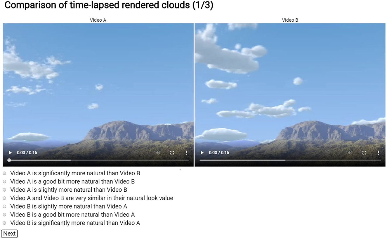
Figure 5. Sample screenshot of the questionnaire page presented to the participants.

All participants had to be 18 years or older to participate in the questionnaire. Since the participants were required to rate the look of different phenomena, choosing participants with normal or corrected to normal eyesight was imperative. They should also have no color deficiencies that could impair their perception of the videos and skew the experiment results. The participants were informed of this on the introductory page, and their consent to participate in this study was obtained.

4. Results

4.1. System Specifications

The method is implemented and tested on a machine with a 4 GHz CPU and an AMD Ryzen 3600, Nvidia RTX 2060 FE GPU at standard clock speed, and 32GB of DDR4 RAM (2133 MHz). All measurements were captured at a screen resolution of 1280 × 720. Each cloud map is stored as a texture on the VRAM memory.

For the preprocessing of source videos into cloud maps, OpenCV was used with Python 3.6.9 through Google Colaboratory (2020c). Figure 6 displays the resulting cloud maps from three different source videos. The solid cloud regions in the source image become nearly mono-colored bright white in the cloud map with little detail, and the clear sky becomes solid black. The cloud maps take a gray shade for the areas where the sky blends with thin cloud sections. However, the resulting cloud maps contain a few gray sections, mostly black or white. The gray sections at the bottom half of the cloud maps contained noise and had some rough edges.

FIGURE 6

Figure 6. Source images (top), perspective corrected and scaled images (middle), and final cloud maps (bottom). Each column represents a different video.

4.2. Machine learning

In Figure 7, the results of three different training configurations can be seen on the cloud data set. These three images were generated after 2,000 epochs of training with a learning rate of 5 × 10⁻⁵. The left-most image is clearly not depicting clouds but could instead be viewed as some form of noise, while the second and third images exhibit a closer resemblance to real clouds. R_DCGAN method not being able to generate clouds meant it could not sufficiently and quickly learn cloud patterns from the amount of data that had been collected. T_DCGAN, however, managed to learn some features of the data set and was, therefore, able to generate images that better resembled natural clouds. This can be attributed to the fact that T_DCGAN has approximately $\frac{1}{24}$ of the number of trainable parameters to that of R_DCGAN, which lets it swiftly learn from small data sets.

FIGURE 7

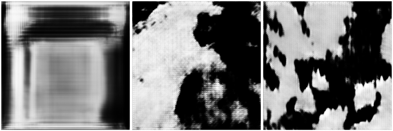
Figure 7. R_DCGAN (Radford et al., 2016) on the cloud data set (left), T_DCGAN (2020b) with perspective correction (middle), and T_DCGAN without perspective correction (right).

The time complexity estimates presented in Table 2 have been calculated based on training using the cloud data set, and they depict the average of over 1,000 epochs of training. This elapsed time represents the average number of seconds the specific configuration runs per epoch for a specific data set resolution. T_DCGAN took roughly 0.67s less time per training epoch compared with R_DCGAN when looking at the three-channel colored images with a resolution of 256 × 256. The difference in training time is most likely due to the difference in the architectural complexity of the models, as more parameters generate more variable changes per operation. However, the results of training on the grayscale data set with a resolution of 256 × 256 show that there is not much difference in the average training times per epoch.

TABLE 2

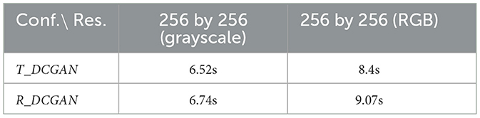
Table 2. Average epoch times of T_DCGAN and R_DCGAN with 1 channel (grayscale) and 3 channels (RGB) for the self-recorded data set.

The minor differences in training time mean a high amount of overhead during the training phase.

Figure 8 presents three columns generated by both DCGAN variants, T_DCGAN (top) and R_DCGAN (bottom), after 0, 1,000, and 2,000 epochs, respectively. The first image in this series, generated with T_DCGAN, exhibits more randomness when compared with the one with R_DCGAN since the former is initialized with Gaussian noise. As the training progresses (second and third columns), we see that the generator for T_DCGAN has learned some significant features and thus converges quickly.

FIGURE 8

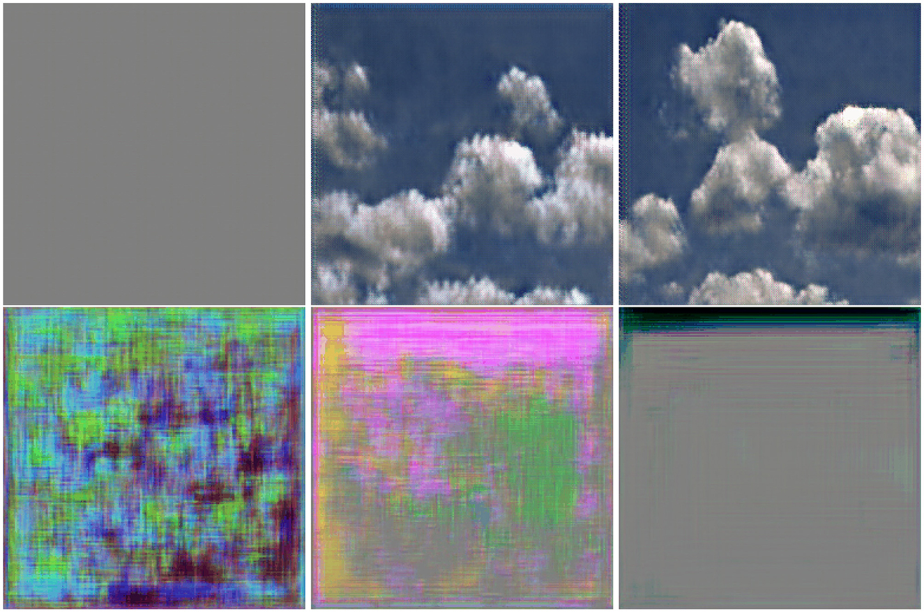
Figure 8. Images generated after 0, 1,000, and 2,000 epochs (columns from left to right, respectively) using T_DCGAN (top) and R_DCGAN (bottom) variants of DCGAN. As shown in Figure 9, R_DCGAN outperforms T_DCGAN at the beginning of training (up until approximately 800 epochs).

4.2.1. FID scores

In Figure 9, the FID scores of both T_DCGAN and R_DCGAN measured over 3,000 epochs can be seen. The cloud data set with three color channels and a resolution of 256 × 256 was used for these measurements. Both these methods start with an initial FID score of approximately 370. The score of the R_DCGAN variant goes down after approximately 800 epochs to a value of 300, which means that the statistics of the generated images are closer to those of the original data set. However, the score, then, goes back up to approximately 370, where it stays for the rest of the training session. The T_DCGAN variant quickly increases from 370 to 550 after 600 epochs. After the 600^th epoch, however, it decreases over time until it reaches a score of sub 140 after 3,000 epochs. As shown, it is trained for more epochs than the R_DCGAN variant, since after 2,000 epochs, it showed a significant improvement over the latter.

FIGURE 9

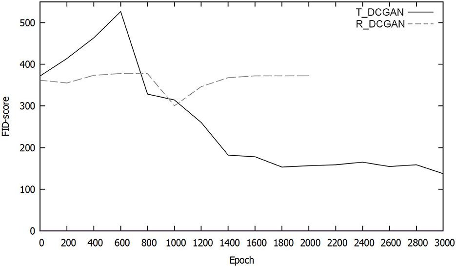
Figure 9. Comparison of the FID scores of T_DCGAN and R_DCGAN variants of DCGAN over time (the lower the FID score is, the better the model).

R_DCGAN showed greater stability at the start of the training. However, this resulted in the model being unable to learn the data quickly enough before it collapsed. T_DCGAN's initial result was worse than that of R_DCGAN. Over time, T_DCGAN improved significantly, reaching an FID score of 137 after 2,000 epochs, and the images generated were more realistic and natural than those of R_DCGAN. After 5,000 epochs of training, the FID score of T_DCGAN had reached 107. From this point onward, we will consider only T_DCGAN for all experiments and analysis, as it emerged as the clear winning candidate. Henceforth, we will cease using the R_DCGAN.

We have trained the models on both data sets, containing pre-processed cloud maps and intact real-life cloud images from the cloud data set. The animations generated using a model trained on cloud maps are shown at the top of Figure 10, while the animations generated using a model trained on real-life cloud images can be seen at the bottom. The grayscale cloud map-based animations retain a lower amount of noise when compared with the three channel-colored animations. This observation can be attributed to the fact that the real-life-based model requires three times as much data as the cloud map-based one since the real-life cloud images have three dimensions per pixel rather than one (i.e., more information needs to be learned).

FIGURE 10

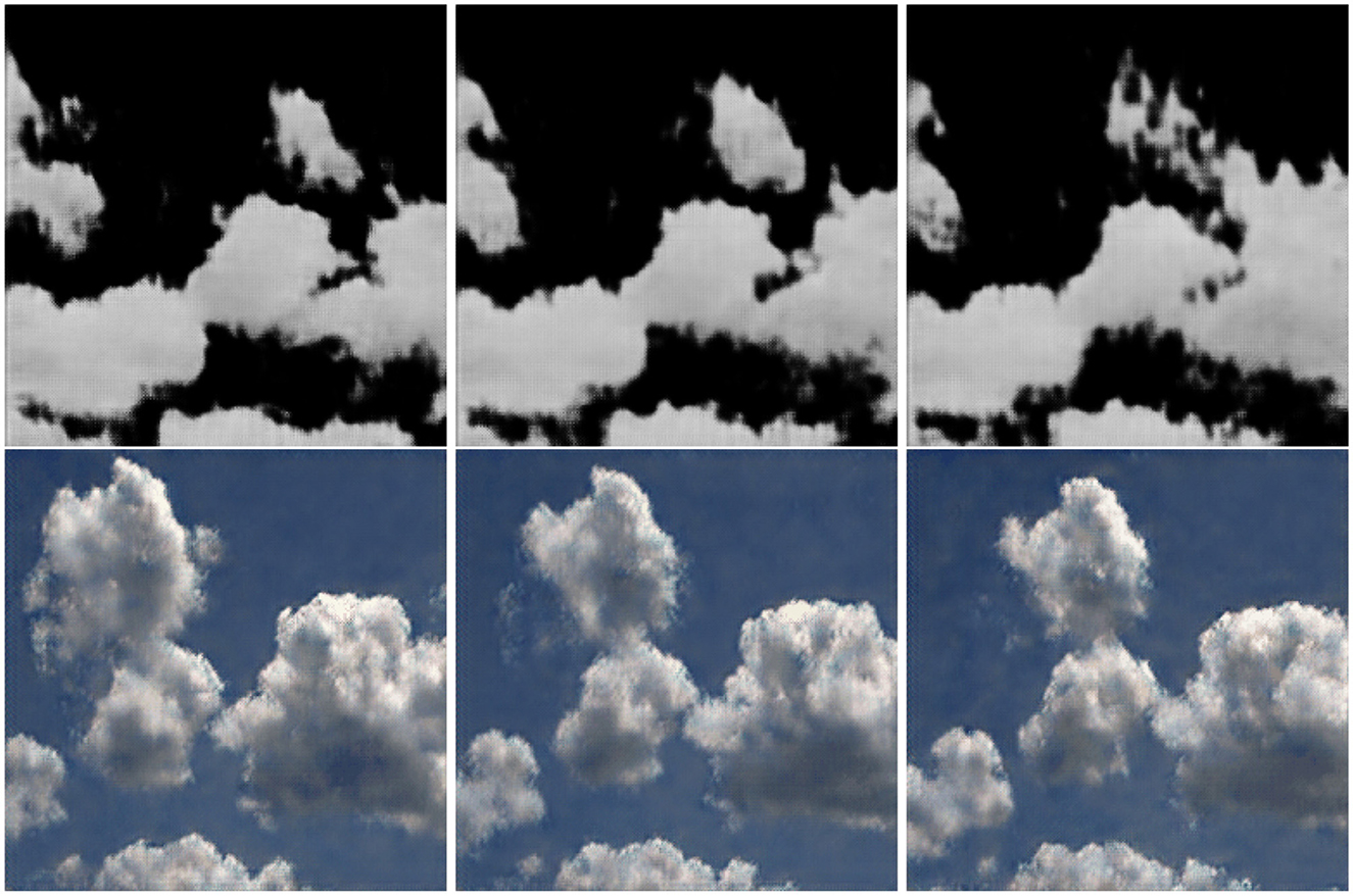
Figure 10. Images generated by models based on T_DCGAN trained on cloud maps (top) and real-life clouds (bottom). Columns represent three different inputs which could be seen as three different timestamps, with no direct correlation to real time.

4.3. Time complexity performance

We plug in our DCGAN-generated cloud maps to the framework by Goswami (2019) and measure the rendering performance. The neural network governs the temporal variation of cloud maps, thereby eliminating the need for any underlying physics. The average execution time of the rendering step was 1.56 ms (see Figure 11, top). Furthermore, an analysis of the graph in Figure 11 (bottom) shows that the execution time of updating the machine learning cloud map is, on average, approximately 1.36 ms per frame. When put in a broader application-sized perspective, a penalty of 1.36 ms is added to each frame. This is an increase of 87% compared with the base execution time for the rendering, assuming all other overheads remain similar. Overall, there is an increase of 6% when compared with the base execution time for the rendering, which makes for a total increase of 93% when combined with the per-frame updating of the cloud map. The total per-frame execution time of the proposed method is an average of 3.02 ms, with the base method sitting at an average of 1.64 ms. Our method would be, therefore, considered interactive in terms of performance. It is worth noting that even though the DCGAN network is learning about and generating cloud maps of resolution 256 × 256, the 3D rendering framework is able to display animating 3D clouds on a screen size of approximately four times larger with the help of these cloud maps.

FIGURE 11

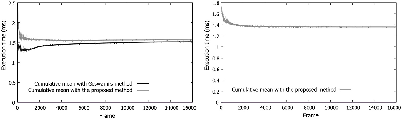
Figure 11. Graphs depicting (left) the execution time of the render step for our approach vs. the base method (Goswami's method, Goswami, 2019) at different frames, (right) the execution time of the machine learning step for the machine learning method.

4.4. Qualitative visual analysis

In Figures 12, 13, we compare the cloud animation obtained by our deep machine learning-based approach against the physics-based method reported by Goswami (2019) for medium and high levels of cloud coverage in the sky, respectively. As stated earlier, we have used the GPU-based renderer in a study of Goswami (2019) to this end, a recent, highly efficient physics-based method. The initial level of cloud coverage is tuned in the renderer, and this first frame is provided as input to the DCGAN. This is important in order to study the different cloud evolutions of the machine learning vs. base method given the same initial cloud state.

FIGURE 12

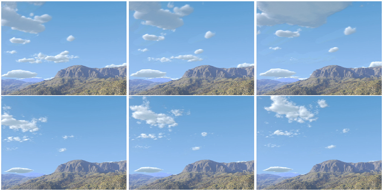
Figure 12. Time-lapse of cloud evolution (medium sky coverage) using (top) the proposed method and (bottom) the base method (Goswami, 2019). Each column represents a 15-s offset in time between adjacent columns, with time increasing from the left to the right.

FIGURE 13

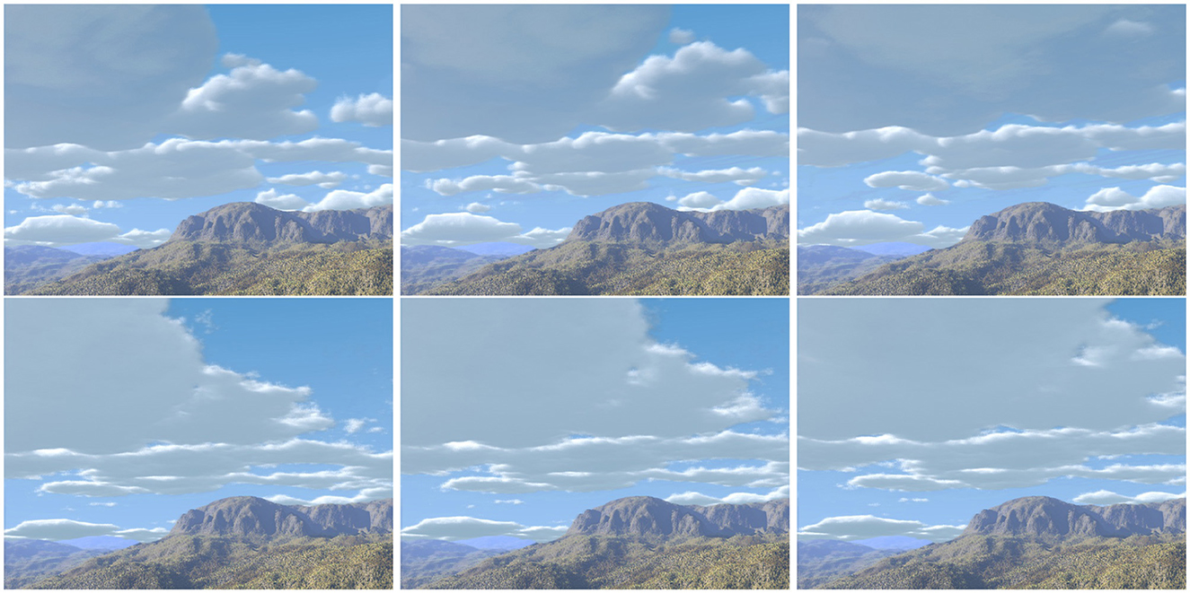
Figure 13. Time-lapse of cloud evolution (high sky coverage) using (top) the proposed method and (bottom) the base method (Goswami, 2019). Each column represents a 15-s offset in time between adjacent columns, with time increasing from the left to the right.

The method of updating the input vectors had an essential role in creating smooth and consistent animations during the experimentation. It is possible to continuously generate animating clouds; however, eventually, a loop would be presented in which the same animation has been played before. Our method can generate animations for a more extended time when compared with a study of Clark et al. (2019), which was only able to generate videos with a few length frames (see videos online).¹

4.4.1. Human perceptual evaluation

Human visual system (HVS) scoring often assesses performance when ground truth data are lacking. For the HVS-based qualitative questionnaire, 41 participants provided their opinions. Of these, 35 were male, 4 were female, and 2 did not specify their gender. Their ages ranged from 19 to 45 years. The seven text-based response options in the questionnaire were mapped to identifying values between “1” and “7”, where “1” would mean being heavily in favor of the base method (Goswami, 2019), “7” being heavily in favor of the proposed method, and “4” being neutral. Among the total 82 answers (for both medium and high cloud coverage sets), 52 votes were in favor of the proposed method, 27 were in favor of the base method, and 3 were in favor of neither of the methods. Figure 14 shows the number of votes for the two comparisons. The most frequently obtained score (a.k.a mode) for the medium cloud coverage was “6,” and for the high cloud coverage, it was “7”. The median was “6” for both comparisons. In other words, the proposed method (machine learning-based) was perceived as more natural than the base method (physics-based) with a score of 69.2 and 62.5% (ignoring the neutral scores) for the medium and high cloud coverages, respectively.

FIGURE 14

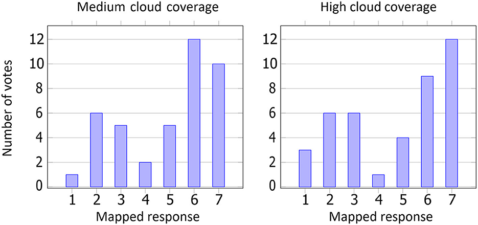
Figure 14. Number of votes per response option in the questionnaire (response options as given in Section 4.4.1). The two comparisons consisted of two videos each, with (left) medium cloud coverage and (right) high cloud coverage, as shown in Supplementary material.

We, furthermore, have quantitatively assessed the videos presented to the participants for visual inspection. The measurements, shown in Figure 15, using BRISQUE and PIQE, validate the performance in favor of the proposed method for the high cloud coverage scenario while having a comparable performance for the low cloud coverage case. Another remark we can infer from these plots is the importance of introducing the perspective correction stage to the overall performance, notably in the high cloud coverage.

FIGURE 15

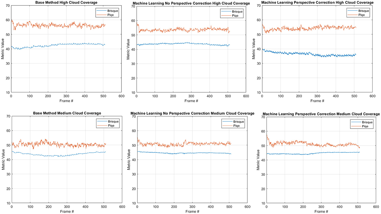
Figure 15. Quantitative quality measurements using known image quality metrics (i.e., BRISQUE and PIQE). The plots depict these measurements calculated for both high and low cloud coverages.

4.4.2. Statistical significance

To test for the statistical significance of users' perceptions favoring either the base method or the proposed method, we conducted a hypothesis testing as follows:

• H0 (null hypothesis): There is no positive shift in the median of observed scoring from the base method to the proposed method at the 1% significance level.

• H1 (alternative hypothesis): There is a positive shift in the median of observed scoring from the base method to the proposed method at the 1% significance level.

As the results from human perceptual evaluation show (Figure 14), the proposed method was considered more natural than the base method for both medium and high cloud coverages. We further conducted a statistical significance test on the obtained participants' responses. Any t-test requires the data to be approximately normally distributed (Japkowicz and Shah, 2011). Since this was not the case for our data, the Mann–Whitney U-test (also known as the Wilcoxon Mann–Whitney test or the Wilcoxon rank–sum test) (Gibbons and Chakraborti, 2011) was used instead. Before determining the statistical significance of the results, the responses are converted to the same range and re-mapped as shown in Table 3. All responses in favor of the base method (response options 1–3) were placed in set A, and their values were flipped according to 4 - X, where X ∈ 1, 2, 3. Similarly, all votes in favor of the proposed method (response options 5–7) were placed in set B and transformed to the range of 1–3 with Y - 4, where Y ∈ 5, 6, 7. Votes in favor of neither the base method nor the proposed method (response option 4) were excluded from the analysis. The two sets, A and B, thus contain exclusive votes in favor of only one of the methods, and the values of the votes represent the strength with which the vote is in favor of that method. To determine the statistical significance of the results, Matlab's rank-sum function was used at the 1% significance level. The statistical significance test, at α = 1%, indicates that there is significant statistical evidence (p = 3 × 10⁻³) to reject the null hypothesis. From this, a conclusion is drawn that there is a positive shift in the median of observed scores from the base method to the proposed method.

TABLE 3

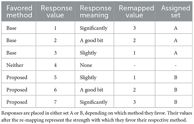
Table 3. Re-mapping of responses obtained from the questionnaire.

5. Conclusion

We have presented an efficient method to generate landscape-scale 3D cloud animation using deep machine learning. Our DCGAN-based approach learns the cloud evolution pattern from simple real-life videos. It can produce realistically evolving clouds at a much higher resolution and interactive frame rates without introducing significant computational overhead. We have employed an efficient preprocessing pass, which helps us to reduce the training time for DCGAN by limiting the size of input images containing cloud evolution information. Nonetheless, the generated output can support a much higher resolution of animation sequences, as demonstrated in the images and videos. We also motivated our choice of DCGAN over other GAN architectures for our problem. We have demonstrated that cloud evolution is easily obtainable purely through machine learning without the use of any underlying physics. Our method circumvents the limitations of most physics-based cloud simulation methods. Whereas the physics-based methods demand a high computational cost and memory storage to provide cloud animation for a limited volume of the sky, our method can easily achieve this animation for a much larger scale and at a higher resolution without very much affecting the frame rates. We have also qualitatively verified our method's improved perceived realism value against the physics-based approach with the help of participants' evaluation.

There are a few promising research directions for our current work. In future, we would like to experiment with our technique to produce animations using other cloud types to produce animations using DCGAN. We would also like to explore the incorporation of lightweight physics to capture certain phenomena that pure machine learning alone cannot capture (saturation level, dew point altitude, etc.). Currently, our method produces cloud animation, which is background invariant. In future, background dependant cloud evolution could be explored with the help of a larger data set. Another promising direction would be to automate the rendering of animated clouds and use artificial intelligence to this end.

Data availability statement

The original contributions presented in the study are included in the article/Supplementary material, further inquiries can be directed to the corresponding author.

Ethics statement

The patients/participants provided their written informed consent to participate in this study.

Author contributions

FJ and SA did a part of this project as their Master's thesis at BTH. All authors contributed to the article and approved the submitted version.

Conflict of interest

The authors declare that the research was conducted in the absence of any commercial or financial relationships that could be construed as a potential conflict of interest.

Publisher's note

All claims expressed in this article are solely those of the authors and do not necessarily represent those of their affiliated organizations, or those of the publisher, the editors and the reviewers. Any product that may be evaluated in this article, or claim that may be made by its manufacturer, is not guaranteed or endorsed by the publisher.

Supplementary material

The videos showing comparison of our approach to the base method are available here. The provided link works better on Firefox browser.

Footnotes

1. ^Video Clips: https://ardisdataset.github.io/Cloud/.

References

Agrawal, A. (2018). Application of machine learning to computer graphics. IEEE Comput. Graph. Appl. 38, 93–96. doi: 10.1109/MCG.2018.042731662

CrossRef Full Text | Google Scholar

Arjovsky, M., Chintala, S., and Bottou, L. (2017). “Wasserstein generative adversarial networks,” in International Conference on Machine Learning (PMLR), 214–223.

Google Scholar

Barbosa, C., Dobashi, Y., and Yamamoto, T. (2015). Adaptive cloud simulation using position based fluids. Comput. Animat. Virtual Worlds 26:367–75. doi: 10.1002/cav.1657

PubMed Abstract | CrossRef Full Text | Google Scholar

Bi, S., Bi, S., Zeng, X., Lu, Y., and Zhou, H. (2016). 3-dimensional modeling and simulation of the cloud based on cellular automata and particle system. ISPRS Int. J. Geoinform. 5, 86. doi: 10.3390/ijgi5060086

CrossRef Full Text | Google Scholar

Borji, A. (2019). Pros and cons of GAN evaluation measures. Comput. Vis. Image Understand. 179, 41–65. doi: 10.1016/j.cviu.2018.10.009

CrossRef Full Text | Google Scholar

Chavdarova, T., and Fleuret, F. (2018). “SGAN: an alternative training of generative adversarial networks,” in Proceedings of the IEEE Conference on Computer Vision and Pattern Recognition (Salt Lake City, UT), 9407–9415.

Google Scholar

Clark, A., Donahue, J., and Simonyan, K. (2019). Adversarial video generation on complex datasets. arXiv preprint arXiv:1907.06571. doi: 10.48550/ARXIV.1907.06571

CrossRef Full Text | Google Scholar

[Dataset] (2016). Cumulus clouds time lapse.

[Dataset] (2020a). Camera calibration and 3D reconstruction.

Google Scholar

[Dataset] (2020b). Deep convolutional generative adversarial network.

Google Scholar

[Dataset] (2020c). Google colaboratory.

Google Scholar

Derrick, B., and White, P. (2017). Comparing two items from an individual likert question. Int. J. Math. Stat 18.

Google Scholar

Dobashi, Y., Nishita, T., and Okita, T. (1998). Animation of clouds using cellular automaton. 251–256.

PubMed Abstract | Google Scholar

Duarte, R. P., and Gomes, A. J. (2017). Real-time simulation of cumulus clouds through skewt/logp diagrams. Comput. Graph. 67, 103–114. doi: 10.1016/j.cag.2017.06.005

CrossRef Full Text | Google Scholar

Eiserloh, S. (2015). Math for Game Programmers: Fast and Funky 1D Nonlinear Transformations.

Ganzoo. (2022). The Gan Zoo. Available online at: https://github.com/hindupuravinash/the-gan-zoo

Gibbons, J. D., and Chakraborti, S. (2011). Nonparametric Statistical Inference. Berlin; Heidelberg: Springer.

Google Scholar

Goodfellow, I., Pouget-Abadie, J., Mirza, M., Xu, B., Warde-Farley, D., Ozair, S., et al. (2020). Generative adversarial networks. Commun. ACM. 63, 139–144.

Google Scholar

Goswami, P. (2019). “Interactive animation of single-layer cumulus clouds using cloud map,” in Smart Tools and Apps for Graphics - Eurographics Italian Chapter Conference, eds M. Agus, M. Corsini, and R. Pintus (Cagliari: The Eurographics Association).

Google Scholar

Goswami, P. (2020). A survey of modeling, rendering and animation of clouds in computer graphics. Visual Comput. 37, 1931–1948 doi: 10.1007/s00371-020-01953-y

CrossRef Full Text | Google Scholar

Goswami, P., and Neyret, F. (2017). “Real-time landscape-size convective clouds simulation and rendering,” in Workshop on Virtual Reality Interaction and Physical Simulation, eds F. Jaillet and F. Zara (Lyon: The Eurographics Association).

Google Scholar

Hädrich, T., Makowski, M., Pałubicki, W., Banuti, D. T., Pirk, S., and Michels, D. L. (2020). Stormscapes: simulating cloud dynamics in the now. ACM Trans. Graph. 39, 1–16. doi: 10.1145/3414685.3417801

CrossRef Full Text | Google Scholar

Harris, M. J., Baxter, W. V., Scheuermann, T., and Lastra, A. (2003). “Simulation of cloud dynamics on graphics hardware,” in HWWS '03 (Goslar: Eurographics Association), 92–101.

Google Scholar

Heinle, A., Macke, A., and Srivastav, A. (2010). Automatic cloud classification of whole sky images. Atmos. Meas. Tech. 3, 557–567. doi: 10.5194/amt-3-557-2010

CrossRef Full Text | Google Scholar

Heusel, M., Ramsauer, H., Unterthiner, T., Nessler, B., and Hochreiter, S. (2017). “Gans trained by a two time-scale update rule converge to a local nash equilibrium,” in Advances in Neural Information Processing Systems, Vol. 30. Available online at: https://proceedings.neurips.cc/paper/2017/file/8a1d694707eb0fefe65871369074926d-Paper.pdf

Google Scholar

Jacobs, N., Abrams, A., and Pless, R. (2013). Two cloud-based cues for estimating scene structure and camera calibration. IEEE Trans. Pattern Anal. Mach. Intell. 35, 2526–2538. doi: 10.1109/TPAMI.2013.55

PubMed Abstract | CrossRef Full Text | Google Scholar

Japkowicz, N., and Shah, M. (2011). Evaluating Learning Algorithms: A Classification Perspective. Cambridge University Press.

Google Scholar

Jhou, W., and Cheng, W. (2016). Animating still landscape photographs through cloud motion creation. IEEE Trans. Multimedia 18, 4–13. doi: 10.1109/TMM.2015.2500031

CrossRef Full Text | Google Scholar

Kallweit, S., Müller, T., Mcwilliams, B., Gross, M., and Novák, J. (2017). Deep scattering: rendering atmospheric clouds with radiance-predicting neural networks. ACM Trans. Graph. 36:1–11. doi: 10.1145/3130800.3130880

CrossRef Full Text | Google Scholar

Karras, T., Aila, T., Laine, S., and Lehtinen, J. (2018). “Progressive growing of GANs for improved quality, stability, and variation,” in International Conference on Learning Representations Vancouver.

Google Scholar

Karras, T., Laine, S., and Aila, T. (2019a). A style-based generator architecture for generative adversarial networks. IEEE Trans. Pattern Anal. Mach. Intell. 43, 4217–4228. doi: 10.1109/TPAMI.2020.2970919

PubMed Abstract | CrossRef Full Text | Google Scholar

Karras, T., Laine, S., and Aila, T. (2019b). “A style-based generator architecture for generative adversarial networks,” in Proceedings of the IEEE/CVF Conference on Computer Vision and Pattern Recognition (CVPR) Long Beach.

PubMed Abstract | Google Scholar

Karras, T., Laine, S., Aittala, M., Hellsten, J., Lehtinen, J., and Aila, T. (2020). “Analyzing and improving the image quality of styleGAN,” in Proceedings of the IEEE/CVF Conference on Computer Vision and Pattern Recognition (CVPR).

Google Scholar

Kazantzidis, A., Tzoumanikas, P., Bais, A., Fotopoulos, S., and Economou, G. (2012). Cloud detection and classification with the use of whole-sky ground-based images. Atmos. Res. 113, 80–88. doi: 10.1016/j.atmosres.2012.05.005

CrossRef Full Text | Google Scholar

Kuhn, M., and Johnson, K. (2013). Applied Predictive Modeling. New York, NY: Springer.

Google Scholar

Lee, Y.-W., and Huh, J.-H. (2020). Evaluation of urban landscape outdoor advertisement signboards using virtual reality. Land 9, 141. doi: 10.3390/land9050141

CrossRef Full Text | Google Scholar

Li, Q., Lu, W., and Yang, J. (2011). A hybrid thresholding algorithm for cloud detection on ground-based color images. J. Atmos. Ocean.Technol. 28, 1286–1296. doi: 10.1175/JTECH-D-11-00009.1

CrossRef Full Text | Google Scholar

Likert, R. (1932). A technique for the measurement of attitudes. Arch. Psychol. 140, 1–55.

Google Scholar

Logacheva, E., Suvorov, R., Khomenko, O., Mashikhin, A., and Lempitsky, V. (2020). “Deeplandscape: adversarial modeling of landscape videos,” in European Conference on Computer Vision (Springer), 256–272.

Google Scholar

Malis, E., and Vargas, M. (2007). Deeper Understanding of the Homography Decomposition for Vision-Based Control, RR–6303. INRIA. p.90.

Google Scholar

Meng, Q., Chen, W., Wang, Y., Ma, Z.-M., and Liu, T.-Y. (2019). Convergence analysis of distributed stochastic gradient descent with shuffling. Neurocomputing 337, 46–57. doi: 10.1016/j.neucom.2019.01.037

CrossRef Full Text | Google Scholar

Mittal, A., Moorthy, A. K., and Bovik, A. C. (2012). No-reference image quality assessment in the spatial domain. IEEE Trans. Image Process. 21, 4695–4708. doi: 10.1109/TIP.2012.2214050

PubMed Abstract | CrossRef Full Text | Google Scholar

Neyret, F. (1997). “Qualitative simulation of cloud formation and evolution,” in Eurographics Workshop on Computer Animation and Simulation (Budapest).

PubMed Abstract | Google Scholar

Park, S.-W., Ko, J.-S., Huh, J.-H., and Kim, J.-C. (2021). Review on generative adversarial networks: focusing on computer vision and its applications. Electronics 10, 1216. doi: 10.3390/electronics10101216

CrossRef Full Text | Google Scholar

Radford, A., Metz, L., and Chintala, S. (2016). Unsupervised representation learning with deep convolutional generative adversarial networks. arXiv preprint arXiv:1511.06434. doi: 10.48550/ARXIV.1511.06434

CrossRef Full Text | Google Scholar

Salimans, T., Goodfellow, I., Zaremba, W., Cheung, V., Radford, A., and Chen, X. (2016). “Improved techniques for training GANs,” in Proceedings of the 30th International Conference on Neural Information Processing Systems, NIPS'16 (Red Hook, NY: Curran Associates Inc.), 2234–2242.

Google Scholar

Schpok, J., Simons, J., Ebert, D. S., and Hansen, C. (2003). “A real-time cloud modeling, rendering, and animation system,” in Proceedings of the 2003 ACM SIGGRAPH/Eurographics Symposium on Computer Animation, SCA '03 (Goslar: Eurographics Association), 160–166.

Google Scholar

Setvak, M. (2003). Time-Lapse Photography of Clouds and Other Atmospheric Phenomena. Available online at: https://www.setvak.cz/timelapse/timelapse.html

Szeliski, R. (2010). Computer Vision: Algorithms and Applications, 1st Edn. Berlin; Heidelberg: Springer-Verlag.

Google Scholar

Um, K., Hu, X., and Thuerey, N. (2017). Perceptual evaluation of liquid simulation methods. ACM Trans. Graph. 36:1–12. doi: 10.1145/3072959.3073633

CrossRef Full Text | Google Scholar

Venkatanath, N., Praneeth, D., Bh, M. C., Channappayya, S. S., and Medasani, S. S. (2015). “Blind image quality evaluation using perception based features,” in 2015 Twenty First National Conference on Communications (NCC) (Mumbai: IEEE), 1–6.

Google Scholar

Vimont, U., Gain, J., Lastic, M., Cordonnier, G., Abiodun, B., and Cani, M.-P. (2020). Interactive meso-scale simulation of skyscapes. Comput. Graph. Forum 39, 585–596. doi: 10.1111/cgf.13954

CrossRef Full Text | Google Scholar

Webanck, A., Cortial, Y., Guérin, E., and Galin, E. (2018). Procedural cloudscapes. Comput. Graph. Forum 37, 431–442. doi: 10.1111/cgf.13373

CrossRef Full Text | Google Scholar

Yuan, C., Liang, X., Hao, S., Qi, Y., and Zhao, Q. (2014). Modelling cumulus cloud shape from a single image. 33, 288–297. doi: 10.1111/cgf.12350

CrossRef Full Text | Google Scholar

Zhang, Z., Li, Y., Yang, B., Li, F. W., and Liang, X. (2020a). Target-driven cloud evolution using position-based fluids. Comput. Animat. Virtual Worlds 31, e1937. doi: 10.1002/cav.1937

CrossRef Full Text | Google Scholar

Zhang, Z., Ma, Y., Li, Y., Li, F. W., Shum, H. P., Yang, B., et al. (2020b). Cumuliform cloud formation control using parameter-predicting convolutional neural network. Graph. Models 111, 101083. doi: 10.1016/j.gmod.2020.101083

CrossRef Full Text | Google Scholar