MeetSafe: enhancing robustness against white-box adversarial examples

Convolutional neural networks (CNNs) are vulnerable to adversarial attacks in computer vision tasks. Current adversarial detections are ineffective against white-box attacks and inefficient when deep CNNs generate high-dimensional hidden features. This study proposes MeetSafe, an effective and scalable adversarial example (AE) detection against white-box attacks. MeetSafe identifies AEs using critical hidden features rather than the entire feature space. We observe a non-uniform distribution of Z-scores between clean samples and adversarial examples (AEs) among hidden features and propose two utility functions to select those most relevant to AEs. We process critical hidden features using feature engineering methods: local outlier factor (LOF), feature squeezing, and whitening, which estimate feature density relative to its k-neighbors, reduce redundancy, and normalize features. To deal with the curse of dimensionality and smooth statistical fluctuations in high-dimensional features, we propose local reachability density (LRD). Our LRD iteratively selects a bag of engineered features with random cardinality and quantifies their average density by its k-nearest neighbors. Finally, MeetSafe constructs a Gaussian Mixture Model (GMM) with the processed features and detects AEs if it is seen as a local outlier, shown by a low density from GMM. Experimental results show that MeetSafe achieves 74%, 96%, and 79% of detection accuracy against adaptive, classic, and white-box attacks, respectively, and at least 2.3× faster than comparison methods.

1 Introduction

Deep neural networks (DNNs) have emerged as highly effective models in machine learning (ML) tasks. Among DNNs, convolutional neural networks (CNNs) revolutionized various computer vision applications, such as medical image recognition (Litjens et al., 2017) and facial recognition (Zhao et al., 2003). However, the robustness of CNNs remains a significant concern, as even a slight and imperceptible perturbations deliberately designed to manipulate images can result in high misclassification rates (Szegedy et al., 2014). Therefore, adversarial detections are in urgent demand to guarantee the integrity of CNN models.

A plethora of adversarial detections (Feinman et al., 2017; Hu et al., 2019; Hendrycks and Gimpel, 2017; Raghuram et al., 2021; Ma et al., 2018; Aldahdooh et al., 2022) have been proposed to identify adversarial examples (AEs). However, these methods remain vulnerable to white-box adversarial attacks (Carlini and Wagner, 2017a; Athalye et al., 2018; Athalye and Carlini, 2018; Tramer et al., 2020), which assume full access to the model and training process. Several defenses (Raghuram et al., 2021; Hu et al., 2019) have been developed against white-box AEs. They obscure the detector's gradients, leading to: (1) diminished security, as gradient obfuscation is proven to be an ineffective strategy for enhancing robustness (Athalye et al., 2018); and (2) inefficient for large CNNs, as computing exact gradients becomes prohibitively expensive.

It has been reported (Hendrycks and Gimpel, 2017; Aldahdooh et al., 2022) that the integration of multiple detections to limit adversary capabilities, a strategy termed “meet the defense”, is promising in countering adversarial attacks. However, these studies did not include any implementation or experimental results. Indeed, exploiting synergistic effects of multiple detections is challenging due to their ineffectiveness. For example, certified methods (Weng et al., 2018; Raghunathan et al., 2018), a widely studied adversarial defense that employs minimum distance decoding (Tramer, 2022) for AEs detection, are generally effective only for AEs with small ℓ_p distances from clean samples. This limitation renders them ineffective against semantically stealthy adversarial examples (Ghiasi et al., 2020), which achieve substantially large but visually imperceptible perturbations by manipulating image factors such as color or shadows. As such, Ghiasi et al. (2020) show that any perturbation on semantic attributes such as shadows is as effective as contrived noise. However, the vast number of semantics in images renders supervised detection inadequate for adversarial attacks (Zheng and Hong, 2018) due to its limited generalization and dependence on patterns specific to the existing dataset.

Meanwhile, many effective adversarial defenses (Zheng and Hong, 2018; Feinman et al., 2017) fail to scale efficiently as CNNs deepen and their number of parameters increases. For instance, the full covariance matrix Σ in I-Defender (Zheng and Hong, 2018) scales as $\mathcal{O}$(d²) w.r.t. the input dimension d of the hidden features extracted by CNN. Similarly, an increase in the number of features exponentially reduces the efficiency of Euclidean distance computations, as noted by Feinman et al. (2017), due to the curse of dimensionality. The complexity of distance calculation also impacts density-based outlier detection methods, such as local outlier factor (LOF) (Breunig et al., 2000), which require repeated distance evaluations between data points and their neighbors in the feature space.

This study proposes MeetSafe, a scalable and effective detection for strong white-box adversarial attacks. MeetSafe selects critical hidden features obtained by convolutional layers, applies feature engineering techniques, and utilizes a Gaussian Mixture Model (GMM) to estimate their distribution. AEs are then identified by the GMM as outliers as they deviate from the distribution of benign hidden features.

In detail, we first observe that the Z-scores of hidden features from selected neurons are non-uniformly distributed (see Figure 1b) in each CNN layer, with not all layers actively extracting features from AEs (see Figure 3a–d). We propose two utility functions to identify the layers most sensitive to adversarial perturbations and the neurons with the largest Z-score differences between benign and adversarial features. By leveraging only the hidden features from the selected neurons, we significantly reduce the feature dimension. Then, our GMM estimates the distribution of selected features processed by three feature engineering techniques: feature squeezing (Xu et al., 2018), which compares the model's predictions on the original and feature-squeezed inputs;whitening (Hendrycks and Gimpel, 2017), captures the principal component of the covariance of inputs; and LOF, which estimates the sparsity of images based on their neighbors in the processed feature space. LOF is ineffective and inefficient in high-dimensional spaces as increased sample distances reduce critical feature impact and raise computational costs for density estimation. To enhance LOF's scalability in high-dimensional feature spaces and reduce statistical fluctuations for improved precision, we propose reachability density (LRD) for local outlier detection. LRD iteratively selects feature subsets with random cardinality and estimate the density of images based on their k-nearest neighbors in the feature space. Finally, an AE is identified if its sparsity, as estimated by the GMM, exceeds the 90th percentile. Experimental results on real-world datasets show that MeetSafe attains a 74%+ detection accuracy against adaptive adversaries, 96%+ against classic adversarial attacks, 79%+ accuracy under white-box attacks, and at least 2.3× faster speed.

Figure 1

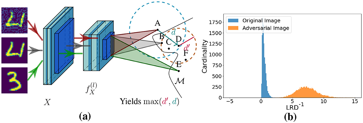
Figure 1. LRD for a MNIST model learned with RCE, utilizing the 10 hidden units with the largest, absolute Z-scores. (a) LRD metric, which uses the averaged maximum of the ℓ₂- (d) and k-distance (d′) among k nearest neighbors. (b) The distribution for test- and FGSM samples with ℓ₂ ≈ 5 and k = 8.

2 Related work

2.1 Notation

A deep neural network can be expressed as the mapping function f^(l)(X):ℝ^m → ℝ^L, where the hidden units at layer l are $f_X^{(l)}\in {ℝ}^L$ for the input X ∈ {𝔇 | 𝔇 ⊆ ℝ^m} in dataset 𝔇. For simplicity, we define units of the last layer of this network (i.e., logits) to be z_i ∈ Z(X) and the predictions to be y_i ∈ Y(X). Neural networks often minimize the empirical risk with a loss function $\mathcal{L}$_f(X) with a batch of ℝ^B×m as input. Our method also utilizes GMMs for detection, which is a linear superposition of Gaussians with the form $\mathcal{N}$(X|μ_i, Σ_i) where Σ and μ denote its covariance matrix and mean, respectively. Each Gaussian has a mixing coefficient π_i that equals the probability p(ξ_i) of a latent variable ξ_i.

2.2 Adversarial attacks

One can define at least three threat models for adversarial attacks: the white-, gray-, and black-box scenario. The white-box setting indicates that the adversary has perfect information about the system. The detector should thus be deterministic for the adversary (Athalye et al., 2018). A weaker assumption is a gray-box model in which the attacker has no knowledge about the defenses. Black-box attacks only assume knowledge of the output and input space, possibly with access to a querying oracle. The empirical risk of an actual threat is often measured with the ℓ_p-norm required by adversarial attacks like the ones below.

2.2.1 Fast gradient sign method (FGSM) (Goodfellow et al., 2015)

FGSM is a one-step ℓ_∞ perturbation toward the gradient of the loss function ∇_X$\mathcal{L}$_f. FGSMs perturbation is ϵ·sign(∇_X$\mathcal{L}$_f), where ϵ is the ℓ_∞ norm of the perturbation. The method assumes linearity in the proximate region of sample X.

2.2.2 Carlini & Wagner (C&W) (Carlini and Wagner, 2017b)

C&W is a first-order constrained optimization that closely resembles Szegedy et al. (2014) method for adversarial example generation. Both define the objective to be $\Vert X{\Vert }_p+c·\widehat{f}(X)$. This objective function includes the ℓ_p distance with a custom criterion $\widehat{f}(X)$, modulated by the sensitivity parameter c and confidence parameter κ. C&W uses $\widehat{f}(X)={({max}_{i\ne t}(z_i)-z_t+\kappa )}^{+}$ where t is the targeted class.

2.2.3 DeepFool (Moosavi-Dezfooli et al., 2016)

DeepFool fits a hyperplane on the target model. The hyperplane is an aggregate of binary classifiers, which encloses the true class k. The algorithm applies Newton's method on the probits to move to the closest non-maximal class t. To misclassify the sample, a small overshoot η is added as scalar.

We describe the perturbations generated by the three methods as near-optimal as they are optimized within the constraints of the ℓ_p-ball. However, recent studies on semantic perturbations have identified approaches that produce adversarial examples more closely aligned with human perception (Luo et al., 2022; Duan et al., 2021; Zhao et al., 2020; Ghiasi et al., 2020). For instance, PerC uses color differences, which considerably increases the ℓ_p distance of adversarial examples. The primary focus in this study is on adaptive near-optimal perturbations on state-of-the-art defenses that do not rely on obfuscated gradients.

2.3 Adversarial detection

2.3.1 Adversarial pockets

A common intuition of adversarial perturbation is that it pushes examples off the manifold of training data. Szegedy et al. (2014) were the first to conjecture the idea with the Lipschitz constant. A high constant enables the manifold to be dense, with low-probability pockets containing adversarial examples. Therefore, generative classifiers may detect these adversarial pockets (Lee et al., 2018; Raghuram et al., 2021; Yin et al., 2019; Feinman et al., 2017; Zheng and Hong, 2018; Li et al., 2019). An example of this is Deep Bayes (Li et al., 2019), which uses a deep latent variable model on the logits to estimate a joint distribution. JTLA (Raghuram et al., 2021) aggregates class-conditional probabilities from each layer by computing kNN class counts. Others trained a more simple GMM (Zheng and Hong, 2018) and utilized Kernel Density Estimation (KDE) (Feinman et al., 2017) on deep layers. Lee et al. (2018) performed a density estimation with the Mahalanobis distance.

2.3.2 Boundary tilting

A geometric analysis renders a different perspective on adversarial examples. When the decision boundary tilts too much toward a submanifold of one class, then the distance of another classification is relatively close. Tanay and Griffin (2016) therefore measured adversarial strength as the deviation angle with a bisecting boundary that maximizes the inter-class distance. This angle can, without major performance hits, be higher along directions of low variance. Near-optimal perturbations may thus be detected by manipulating such components with semantic-preserving image filters (Xu et al., 2018; Tian et al., 2021; Liang et al., 2018). In particular, feature squeezing (Xu et al., 2018) uses median smoothing and bit-depth reduction. Tian et al. (2021) train a dual model on the sample's wavelet transform. Others (Song et al., 2018; Hu et al., 2019) propose denoisers which perturb samples with optimizers. Scene statistics may also detect the perturbation, like whitening (Hendrycks and Gimpel, 2017) that measures the variance of low-rank eigenvectors. Li and Li (2017) also use low-rank eigenvectors with their extremal value to detect extreme deviations, both (Kherchouche et al., 2020; Akhtar et al., 2018) train simple classifiers on BRISQUE's (Mittal et al., 2012) features, and Local Intrinsic Dimensionality (LID) (Ma et al., 2018) directly calculates the dimensionality. However, current adversarial detection methods are ineffective at identifying hidden anomalies in high-dimensional spaces and are not efficient for large dataset.

Contributions of this study are as follows: (i) We propose MeetSafe, a scalable detection algorithm for adaptive adversarial examples. (ii) Two utility functions that allow LRD and other detectors to scale based on a unit's Z-scores or rate of change under perturbation. (iii) Extensive empirical evaluations on 4 datasets and 14 models that show effectiveness of whitening and MeetSafe under adaptive white-box attacks.

3 Method

The main idea of MeetSafe is to combine discrepant detectors in an ensemble. In particular, we use the scores of whitening (Hendrycks and Gimpel, 2017), feature squeezing (Xu et al., 2018), and a density estimation, called LRD, within a GMM. LRD makes two novel improvements on existing density estimates. First, we noticed that the activation's Z-score of hidden features is not uniform under perturbation (see Figure 1b); we therefore use two utility functions to select the 10 units that were most anomalous under perturbations. Second, kernel density estimation does not adjust for local densities, which carries the risk of over-smoothing as illustrated by Ma et al. (2018). Like Ma et al., LRD uses an extension of the k-distance.

We now turn to LRD and its relation to non-parametric methods. Then, we explain the used features and feature selection of LRD. Finally, this section introduces MeetSafe.

3.1 Density estimation with k-distances

Non-parametric methods model the distribution p(X) with limited assumptions for the true distribution. This makes the models flexible. Distribution p(X) can, for instance, be generalized with its volume V and cardinality K of X's proximite region, given enough observations. In contrast to KDE, the kNN method fixes the cardinality and finds the appropriate volume from the data. For a sample X, one can then estimate p(X) using the frequentist notion:

$\begin{array}{ll}\widehat{p}(X)=K/(|𝔇|·V)& (1)\end{array}$

where the dataset 𝔇 is sampled from p(X). The volume is defined by a sphere with the k-distance as radius, which makes the k-distance of a test sample X sufficient to approximate p(X). The estimate would only be shallow with limited information from its neighbors. Recursive calls on neighbors may improve the estimate due to greater depth.

Notice that BRISQUE hidden features may be affected by unequal standard deviations as these are not normalized. Some have thus more influence on the k-distance than others. This is not favorable, especially because we stated earlier that the low variance components may be an important characteristic of some adversarial examples. Our method will therefore use the scaled Euclidean distance. This normalizes the k-distance with respect to a diagonal covariance matrix Σ. In addition, we will lower the memory burden of the kNN algorithm in Section 3.2, after we discuss the details and idea of LRD.

3.1.1 Local reachability density (LRD)

The intuition behind LRD comes from Breunig et al. (2000), in which they propose LOF, a heuristic for finding local outliers. LRD extends the k-distance as it smooths out statistical fluctuations in at least two ways. First, the actual distance, called reachability, used to estimate the volume V is capped by the k-distance of the neighbor. Second, the average is taken among the k nearest neighbors. The reachability measure reach(X₁, X₂) of two nodes (A & D) is demonstrated in Figure 1, and the value depends on the volume of node D and its Euclidean distance to A. Whichever value is bigger equals the reachability from D to A:

$\begin{array}{ll}max\left[\begin{array}{c}{\displaystyle d_{X_2,k}^{\prime }},\sqrt{{(X_1-X_2)}^T{\Sigma }^{-1}(X_1-X_2)}\end{array}\right]& (2)\end{array}$

where d′ is the k-distance. Substituting the reachability from A to its neighbors N_A in Equation 1 yields its reachability density (Equation 3). Using reachability as a measure to assess the density in the proximate region of node A has the advantage that only a fixed amount of neighbors needs to be considered.

$\begin{array}{ll}LRD(X)=|{\text{N}}_X|/({\displaystyle {\sum }_{n_i\in {\text{N}}_X}}reach(X,n_i))& (3)\end{array}$

We add one novel improvement called feature bagging (Lazarevic and Kumar, 2005). This enables LRD to capture higher dimensions. The generalizability of kNN degrades under these circumstances, as the distance between all data points becomes larger and individual features have less of an impact. Bagging is a popular approach to limit this issue. It takes a subset (with random cardinality) of the features for multiple iterations and returns a combined LRD score.

3.2 Feature engineering for LRD

We now consider two possible Points Of Interests (POI) for LRD: the layer after convolution and the pixel values, where we refer to the former as Learned Feature Analysis (LFA). Specifically, we explain how we select its features for both options as without limiting its feature space, LRD would be space inefficient and suffer from sparse data.

On raw pixel values, we advise the use of BRISQUE. BRISQUE fits a Gaussian-like distribution on the raw image while maintaining structural information, which can evaluate the naturalness of an image. Moreover, BRISQUE is 149 times faster than wavelet methods such as DIIVINE and performs almost similar on white noise (Mittal et al., 2012).

On hidden layers, we extract a random set of hidden features. Depending on the chosen POI, the Z-scores of FGSM examples X′ will be used to select the best 10 features of BRISQUE or the best 10 hidden features. We will further explain this feature selection more formally.

3.2.1 Selecting hidden features

For the hidden features f^(l), a pool $\mathbf{P}{\subseteq }_R{f}^{(l)}$ is defined, so that its members are chosen randomly at initialization and preserved during execution. The detector then follows a watching scheme upon $\mathcal{P}$ and its utilities (Equation 4, 5). The first equation calculates the difference in Z-scores of all features in the pool. It estimates the units that were relevant under perturbation. The second estimates the rate of change of one layer. The first utility is calculated with FGSM after every epoch, and this is the fastest evasion method we know, limiting the constraints on scalability or parameter updates. The second utility showed most potential in the final layers, making that our preferred choice (Section 5.1). Because of this, we believe the second utility is optional.

$\begin{array}{ll}{U}_{\mathcal{P}}=\frac{1}{|𝔇|}{\displaystyle {\sum }_{X\in 𝔇}}\frac{|{\mathcal{P}}_X-{\mathcal{P}}_{X^{\prime }}|}{{\sigma }_{\mathcal{P}}}& (4)\end{array}$

$\begin{array}{ll}{U}_{f^{(l)}}=\frac{\Vert E_{X~𝔇}\left[f_{X^{\prime }}^{(l)}\right]-E_{X~𝔇}\left[f_X^{(l)}\right]{\Vert }_2}{\Vert E_{X~𝔇}\left[f_X^{(l)}\right]{\Vert }_2}& (5)\end{array}$

3.3 MeetSafe

Our MeetSafe combines LRD, using hidden features as POI, with variance-based anomaly detection—whitening (Hendrycks and Gimpel, 2017)—and feature squeezing (Xu et al., 2018) in a GMM, for which an ablation study is given in Section 4.3. The scores of the three heuristics are learned through Expectation-Maximization (EM).

$\begin{array}{ll}-log\widehat{p}(X)=-log\left[\begin{array}{c}\sum ^K{\pi }_i·\mathcal{N}({\mathcal{H}}_X|{\mu }_i,{\Sigma }_i)\end{array}\right]& (6)\end{array}$

Concretely, to detect a sample, we first select the best features based on U_{$\mathcal{P}$} for LRD and the eigenvectors of the training data (Algorithm 1). Then, we evaluate the three heuristics (denoted as $\mathcal{H}$_X). Assuming normality, a three-dimensional GMM fitted on benign data can classify the sample as malicious when it exceeds the 90th percentile of the Equation 6. The workflow of MeetSafe is shown in Algorithm 2.

Algorithm 1

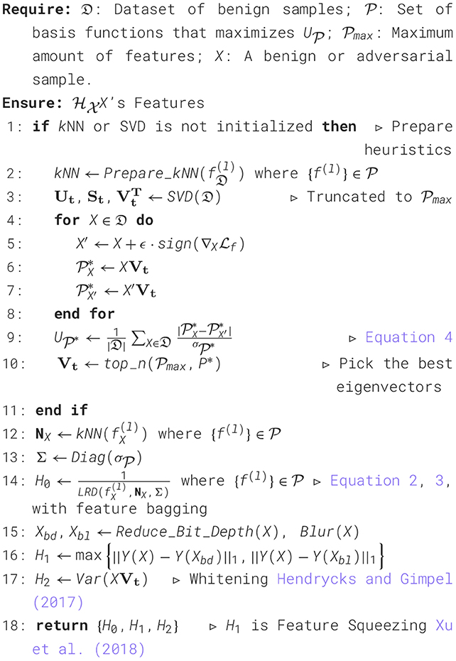
Algorithm 1. MeetSafe's feature extraction.

Algorithm 2

Algorithm 2. MeetSafe.

4 Experiments

We evaluate MeetSafe and LRD against several adversarial attacks including FGSM, DeepFool, and C&W. The experiments will demonstrate white- and/or gray-box performance for four datasets: Tiny-ImageNet (Le and Yang, 2015), CIFAR-10 (Krizhevsky and Hinton, 2009), MNIST (LeCun, 1998), and STL-10 (Coates et al., 2011). Only for Tiny-ImageNet, we resized the samples to be in ℝ^3×64×64. The attacks are restricted to an ℓ₂ distance to ensure a fair comparison across datasets and ℓ_∞-based methods. For instance, an ℓ_∞ distance permits more noise for higher resolution images. Consequently, we use the ϵ parameter given by Equation 7, so that the maximum allowed perturbation of FGSM equals that of ℓ₂ methods (δ_max); where the image X is given by a ℝ^m flattened matrix.

$\begin{array}{ll}ϵ=\sqrt{\Vert {\delta }_{\text{max}}{\Vert }_2^2/m}& (7)\end{array}$

Each attack, defense, and target model is re-implemented in PyTorch. Herewith, we evaluated 14 models based on ResNet-50 (He et al., 2016) and VGG-13 (Simonyan and Zisserman, 2015). Ten of them are trained with robust optimization techniques, utilizing gradient smoothing (RCE) (Pang et al., 2018) or adversarial training with FGSM (ℓ₂-radii of 5) (AL) (Goodfellow et al., 2015).

The experiments also include some related methods that will be compared to MeetSafe and LRD. The baseline for MeetSafe (MS) is KDE with predictive uncertainty (KDE+BU) (Feinman et al., 2017), I-Defender (I-Def) (Zheng and Hong, 2018), and the Mahalanobis measure (MAH) (Lee et al., 2018). Additional work that we tested are LID (Ma et al., 2018), Whitening (PCA) (Hendrycks and Gimpel, 2017), Feature Squeezing (FSQ) (Xu et al., 2018), extremal value (EXM) (Li and Li, 2017), and Kherchouche et al. (2020)'s third model for BRISQUE (SVM).

4.1 Experimental setup

We trained the models for 150 epochs on predetermined training sets. During training, a batch size was used of 256, learning rate of 0.01 with momentum 0.9 under a cosine annealing schedule, and 1e − 4 weight decay. The model is also adapted to exhibit required invariances. All training samples are normalized on each channel, randomly flipped horizontally, and randomly cropped within a padding of 4. Adversarially learned models were additionally trained half-on-half on benign and perturbed data.

We evaluated the detectors on unseen test images and their perturbed variants as follows. First, we evaluate the defense and model on non-adaptive gray-box perturbations. That includes the one-step FGSM perturbation as well as the DeepFool and C&W-ℓ₂. Second, for each defense, we evaluate its best-performing technique (RCE or AL) on DeepFool against adaptive white-box attacks.

White-box attacks can be generated by adding the detector's likelihood function (Equation 6) to C&W's objective (Carlini and Wagner, 2017a). In essence, this optimizes a multi-objective gradient with Adam that considers both the gradient of the detector's internals and the confidence of the target model:

$\begin{array}{ll}\Vert X{\Vert }_p+c·\widehat{f}(X)+c^{*}·{(-{\tau }^{-1}log\widehat{p}(X)-1+\kappa )}^{+}& (8)\end{array}$

where τ is a given threshold and c^* a constant that controls the sensitivity toward the detector's gradient, optimized with binary search. The sample is updated with perturbation δ when its aggregate X + δ fools successfully. For our experiments, we limit the perturbation to a ℓ₂ distance of 5.

Our white-box attack follows an all-or-nothing criterion: the batch with adversarial examples is either clean or fully successful. For this reason, we assume that the detector is successful if either the white-box perturbation is detected or classified by the target model. Its true positives are thus in the set $\left\{X|\text{ argmax }Y(X)\ne k\vee -log\widehat{p}(X)\le \tau \right\}$ for true class k and threshold τ.

The performance of the defenses is measured using its overall detection accuracy of one test run in both adversarial and benign situations, where the detector classifies at a TNR of 90%+. The adversarial setting may include samples without perturbation when the target model already misclassifies the clean sample. We therefore have an optimal detection accuracy of $1-\frac{{\mathbf{R}}_f}{2}$ with standard empirical risk $\mathcal{R}$_f of the target model.

During test runs, we reduced the batch size to 128 (64 for white-box); other hyperparameters, used for the attacks and defenses, were as follows. The magnitude ϵ of FGSM is deduced from Equation 7, DeepFool had an overshoot of 0.02, and C&W executed 5 steps with 500 iterations (10 and 1000 for white-box) under a 0.05 confidence κ. For all defenses, we applied the same feature selection. That took the best 10 in a pool of at most 500 features, given U_{$\mathcal{P}$}. We choose the k of kNN to be 8 for LRD and LOF based on the ablation study in Sec. 5.3. See Section 5.3 for details. The experiments were conducted on AMD Ryzen 7 7700X and Nvidia RTX 4070 Ti.

4.2 Model performance

The accuracy of the models is shown in Table 1. The CIFAR-10 ResNet-50 model is able to reach an average cross-entropy of 0.0249 and a test accuracy of 93.2%. The cross-entropy for robust optimization techniques is notably higher, and this increased to 0.47 for adversarial training and 431.1 for RCE. A higher value for RCE was expected as almost each class now adds to the error instead of only the true class. We also observe that the fit and convergence changes dramatically when the amount of classes is increased. Take Tiny-ImageNet which has 200 classes, where the others have 10, a RCE model trained on ImageNet does only reach an accuracy of 3%. When we test the STL-10 subset, RCE does not show this behavior.

Table 1

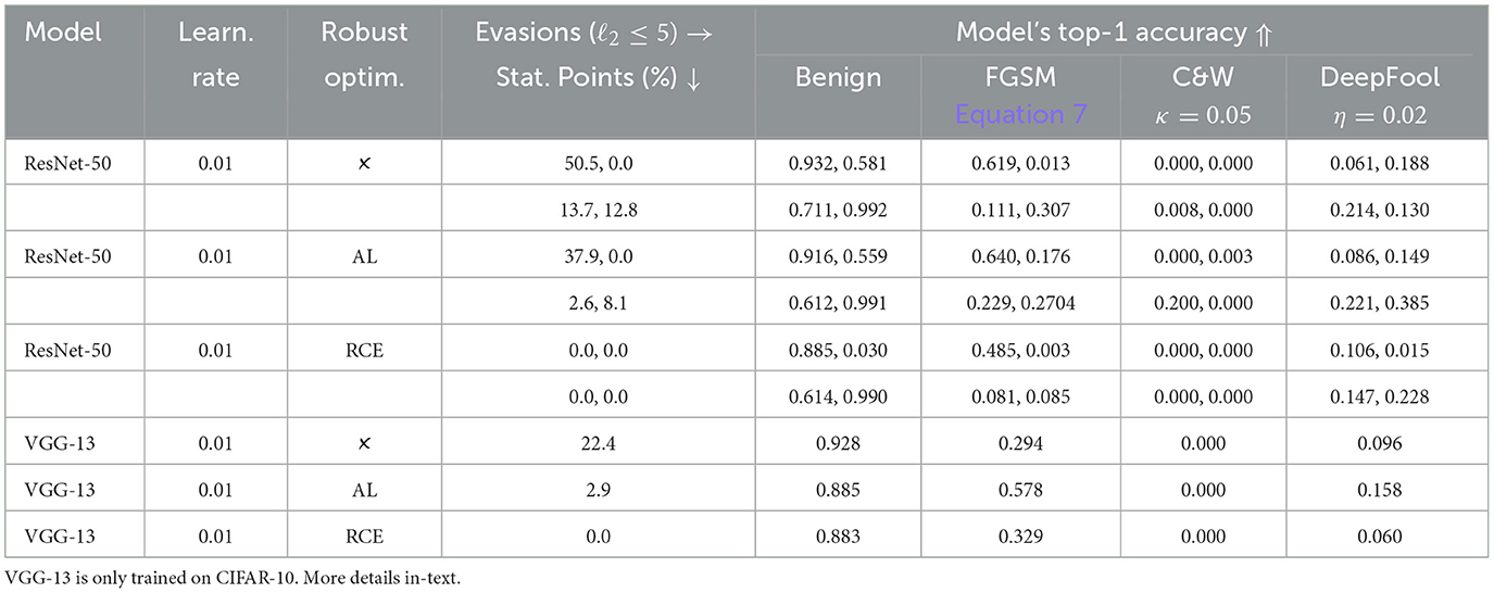
Table 1. Accuracies and proportion of stationary points for FGSM of the trained target models on the CIFAR-10, Tiny-ImageNet, STL-10, and MNIST testing set, respectively.

Robust optimization shows a descent mitigation of FGSM for all models and no meaningful mitigation of C&W attacks. The results of DeepFool show that the optimized models are often more robust than the plain ones under smaller perturbations. Still, the high adversarial accuracy of the plain model is somewhat unexpected. However, this may have a clear reason. Namely, the confidence of this model is higher, which causes vanishing gradients.

4.2.1 Vanishing gradients

The confidence score of the plain ResNet-50 is near a unit vector toward the correct class for some images (Table 1), which makes that gradient zero due to rounding errors. Such images sit on a stationary point for the current parameters. This is a major drawback of FGSM, but not present for DeepFool and C&W which use gradients of different loss function. Vanishing gradients do give a sense of robustness for the plain model, while it is probably not.

4.2.2 Utility of hidden layers

The utilities discussed in Section 3.2 grow more or less each layer for the CIFAR-10 ResNet. The RCE and plain model exhibit the largest normalized ℓ₂ distance at the fourth bottleneck and the smallest distance at the raw input. The utility $U_{f^{(l)}}$ at the first and last bottleneck differs significantly with RCE; as for 5 samples, the 95% t-confidence interval (CI) is 0.29 ± 0.003 and 0.51 ± 0.01, respectively. This supports the unfolding intuition of Bengio et al. (Bengio et al., 2013). Although, we find the behavior of adversarial learned models to be different. There, the first layers seem to be the most sensitive, with the first bottleneck (0.66 ± 0.14) having a higher utility than the fourth (0.48 ± 0.13). Detection methods may thus be fine-tuned by utilizing different layers.

4.3 Detection results

The following section will primarily discuss the performance on near-optimal perturbations. We showcase more results in Section 4.1 regarding the accuracies under semantic adversarial attacks such as shadow attack (Ghiasi et al., 2020) and PerC (Zhao et al., 2020).

4.3.1 Against gray-box attacks

We start by examining gray-box attacks on CIFAR-10. This provides a more comprehensive understanding of our method's performance. Table 2 shows LRD in addition to various other works. Instance-based methods similar to ours are KDE+BU, LID, and MAH. We see that LID does not lead to practical results. On the other hand, LRD reaches an accuracy above 85% for FGSM perturbations, and this outperforms similar methods.

Table 2

Table 2. Accuracies of several detection algorithms against gray- and white-box (GB/WB) adversaries with a ℓ₂-radii of 5.

We also consider Robust optimization beneficial. The detection accuracy is frequently higher with one of these methods. Particularly for PCA, its accuracy against DeepFool and FGSM shows a respective difference of 15% and 26%. Moreover, PCA shows strong and similar results as the supervised method SVM on FGSM; the extremal measure, that also uses PCA, is less effective. Finally, we consider feature squeezing's performance limited for FGSM perturbations. It achieves the lowest accuracy of 76% after LID.

These results largely change for smaller perturbations. SVM drops from 90%+ accuracy to a random classifier. In fact, almost all methods suffer from smaller perturbations, except for purification measures such as feature squeezing. Its situation is reverse for smaller perturbations and does improve in this setting, which suggests that most methods do not have a sufficient scope to cover all adversarial attacks.

4.3.2 Against adaptive attacks

We test MeetSafe against adaptive adversaries, a challenging AEs detection scenario, and also show in Table 3. We find that an adaptive attacker can break most methods. In particular, the results for KDE+BU, LID, EXM, and MAH showed a true positive rate close to 0% on the CIFAR-10 and STL-10 datasets, which is consistent with prior works (Carlini and Wagner, 2017a; Athalye et al., 2018).

Table 3

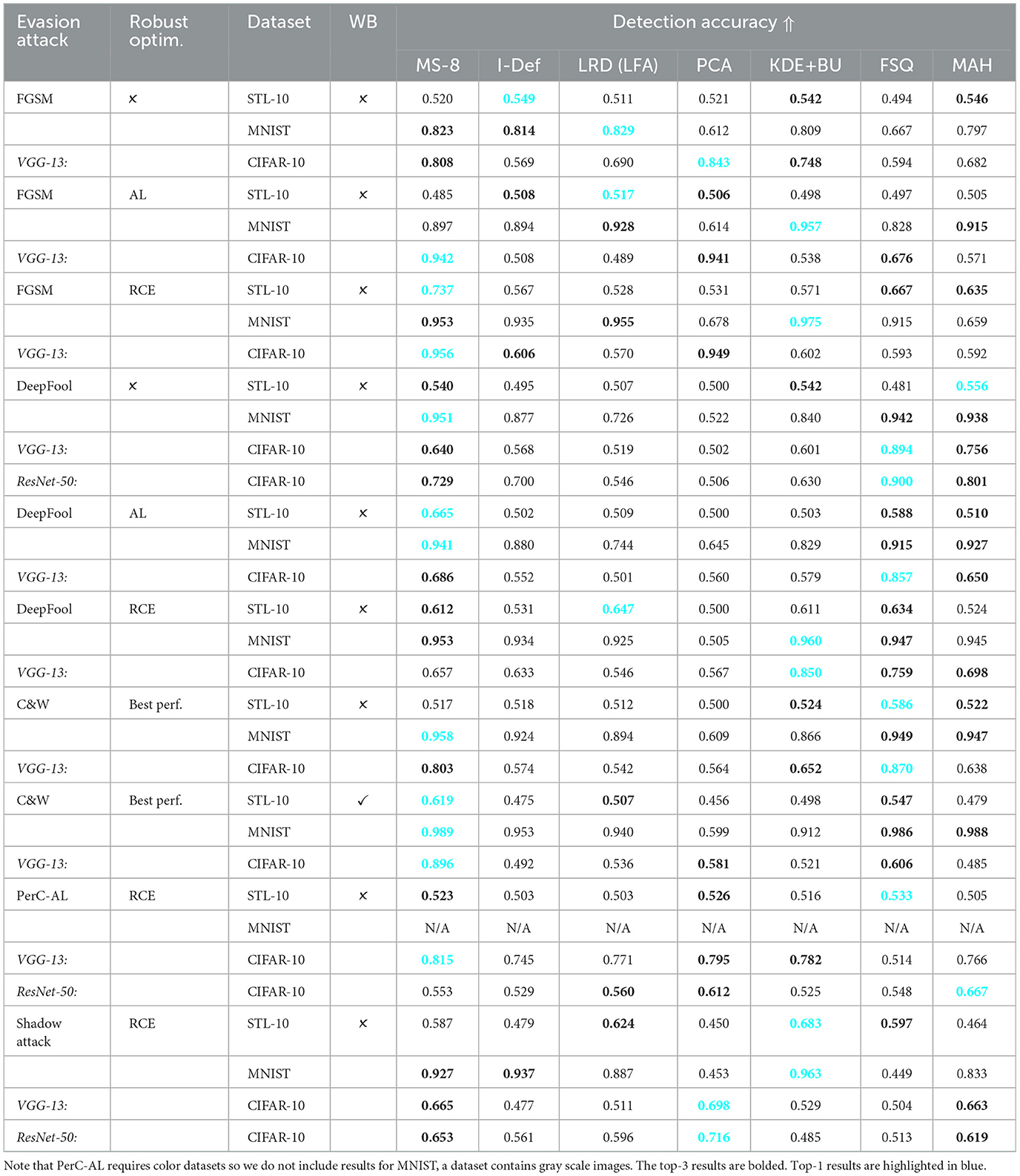
Table 3. Accuracy of comparison detections evaluated against gray- and white-box (GB/WB) adversaries on STL10, MNIST, and CIFAR10; with a ℓ₂-radii of 5.

Regarding the other methods, we see that especially PCA excels with accuracies of approximately 80% for CIFAR-10. Surprisingly, PCA was proven as not robust earlier (Carlini and Wagner, 2017a). LRD is, in addition to PCA, also somewhat resilient against adaptive attacks, although it should be noted that BRISQUE does utilize local non-linear operations to estimate generalized gamma functions (Mittal et al., 2012), which are not smooth functions. We can therefore only consider LRD robust on the hidden features. Some results are worse than in the gray-box setting, that is possible due to the positive confidence value. Hence, the adversarial example is stimulated to be 5% below the detector's threshold, which improves its transferability on models with feature bags or other uncertainties.

We show the performance of LRD, PCA, and FSQ and their MeetSafe ensemble across datasets in Table 2. The p-values of the methods' confidence are computed and compared against a threshold. Specifically, we evaluate the p-values for 10 random FGSM samples using a reversed ResNet-50 model trained on a benign dataset. A low p-value is beneficial for the GMM's generalization as this assumes normality. On MNIST, an opposing utility between LRD and whitening techniques becomes clear. Here, LRD has a p-value of near zero (≤10⁻⁹⁹), while whitening has a value of 6e-6. On the other hand, whitening performs relatively better on CIFAR-10 with a p-value smaller than 1e-80 against 5e-17 for LRD. Whitening and LRD might therefore offset each other's effects against FGSM.

The added value of feature squeezing is apparent for small CIFAR-10 perturbations. Figure 2a shows the performance of the three detectors for DeepFool and FGSM. It shows a noticeably higher AUROC for feature squeezing on DeepFool. Furthermore, feature squeezing has the smallest p-value of 0.01, followed by LRD with 0.25. Feature squeezing could thus be helpful in the case when the adversarial sample is near the benign input. Section 5.2 discusses the importance of each components of MeetSafe.

Figure 2

Figure 2. (a) ROC curves of MeetSafe's features on CIFAR-10 and a reverse ResNet-50 as target model. The curves show the performance against DeepFool and FGSM. (b) Graph that shows the inference times of MS-8 and a reversed ResNet-50 on MNIST, CIFAR-10, Tiny-ImageNet, and STL-10. The error bar denotes the t-CI across 5 runs.

4.3.3 GMM-based detection

Our MeetSafe constructs a GMM-based detection with PCA, feature squeezing, and LRD. We test MeetSafe's performance under certain number of Gaussian components: 4, 8, and 16 (Table 4). For gray-box perturbations, we see that only 4 components may be useful for FGSM, but this increases for small perturbations. To balance these accuracies, we think that 8 components are desirable. Comparing the performance of MS-8 to that of I-Defender shows similar results on FGSM, but lower accuracies on stronger attacks. Meanwhile, the accuracy for RCE and MeetSafe does not scale well. This is most notable when we compare the efficacy for datasets of higher resolution. Tiny-ImageNet shows accuracies on C&W of at most 0.553 for MeetSafe and 0.511 for I-Defender. STL-10 shows similar results (Table 4). However, the effect of dimensionality is not a limitation specific to our method but rather a general issue of defenses against AEs (Goodfellow et al., 2015). MS-8 achieves an improvement of at least 8.1% on adaptive attacks and 10.2% on the worst-case results for each evaluated method by averaging across STL-10, MNIST, and CIFAR-10. MeetSafe may therefore be employed universally while maintaining a considerable detection accuracy.

Table 4

Table 4. Accuracies of GMM-based detectors against gray- and white-box (GB/WB) adversaries with a ℓ₂-radii of 5 like in Table 2.

Table 5

Table 5. Accuracies of GMM-based detectors against gray-box adversaries on Tiny-ImageNet, STL-10, and CIFAR-10, with a ℓ₂-radii of 5.

4.3.4 Inference time

Figure 2b shows the inference time of MeetSafe and a ResNet-50 target model on four datasets: MNIST, CIFAR-10, Tiny-ImageNet, and STL-10. Plotted according to the input size of one sample: 784, 3, 072, 12, 288, and 27, 648, respectively. From the figure, we can observe that the discrepancy of ResNet-50 and MeetSafe converges to a factor of approximately 2.3 when the input size gets larger. We increased the feature size from 10 to 17 and the pool size from 500 to 850. We anticipated that this would lead to increased computation, especially for LRD. The results on CIFAR-10 demonstrate that this increase led to a slower processing rate, with the model running 0.28 batches per second slower than before. We consider this change to be limited, indicating that the computational overhead is also manageable given the increased feature and pool sizes.

5 Ablation study

5.1 Sensitivity and utility of the hidden layers

Figure 3 explores the $U_{f^{(l)}}$ utility in the study. The barplots show the utility at the outputs of that layer, which tends to increase when the perturbed sample traverses deeper layers, but this may come with fluctuations. For instance, the values for the STL-10 models seem to decrease in the last layers. The adversarial learned CIFAR-10 model also decreases in utility after the first bottleneck. Still, the final bottleneck remains in the Top-3, suggesting its pivotal role in model performance and feature extraction. Conversely, the initial convolution, denoted as “conv1”, frequently exhibits the least utility.

Figure 3

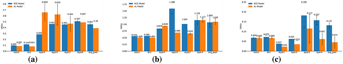
Figure 3. Average of normalized Euclidean distance between FGSM AEs (ℓ₂ of 5) and benign samples under $U_{f^{(l)}}$ at each ResNet-50 layer. The error bars denote the 95% t-CI across 5 runs. (a) CIFAR-10 dataset, (b) MNIST dataset, and (c) STL-10 dataset.

We also see a major difference in the CI's critical region of the CIFAR-10 models. Specifically, the adversarial learned model displays notable variability on each layer, especially when compared to the RCE model. That is in line with the narrow activations in the scatterplots of Figure 4. The RCE models exhibit greater utilities in its deeper layers. Consequently, we anticipate enhanced performance when these hidden units are utilized for detection purposes. Otherwise, adversarial learning would become more intriguing due to the improved model accuracy (see Table 1).

Figure 4

Figure 4. Activations' Z-Score of three hidden features before and after an FGSM perturbation, with a ℓ₂-radii of 5. The activations are sampled from a random pool of 500 hidden features, directly after convolution. We show the activation of hidden features with the highest and lowest Z-score in (a, b) for an adversarially trained ResNet50 on CIFAR10 and non-adversarially trained results in (c, d).

5.2 On the impact of MeetSafe components

We check the detection performance by removing each component of MeetSafe (MS-8) to establish its importance within the ensemble. For the ablation, we trained 3 GMMs all with two components (LRD, PCA, FSQ) on a reversed ResNet-50 and CIFAR-10. First, when we remove LRD the accuracy decreases by 0.054 for C&W, −0.027 for FGSM, and 0.117 for DeepFool. For FGSM perturbations, the results do show that LRD does not add much for on CIFAR-10, as its ablation leads to equivalent accuracies of the GMM. Overall, LRD increases the effectiveness of MeetSafe across various scenarios, aligning with the findings presented in Section 4.3. Second, when we remove PCA, the accuracy decreases by 0.191 for C&W, 0.234 for FGSM, and 0.145 for DeepFool. Whitening is thus an important component on CIFAR-10. Third, when we remove FSQ, the accuracy decreases by 0.197 for C&W, −0.048 for FGSM, and 0.137 for DeepFool, which is also in line with the results in Section 4.3.

5.3 On the impact of k for kNNs

To determine the optimal k, we evaluated the accuracy of LOF and LRD using features from a random pool of 500 hidden features, as shown in Figure 5. The left axis represents LRD accuracy, while the right axis denotes LOF accuracy. The results are plotted separately to highlight their distinct trends, each spanning an accuracy range of 0.06. The elbow points indicate an optimal k = 8 for both methods, which we adopt for all k-NN-based approaches. Notably, LRD achieves significantly higher accuracy than LOF, and k impacts LOF more than LRD.

Figure 5

Figure 5. Performance of LOF and LRD under different k with the amount of feature bags t=30 under CIFAR-10 and adversarial learned ResNet-50.

6 Conclusion and limitation

This study present MeetSafe, a scalable and effective framework to detect white-box AEs. By leveraging insights from feature distribution irregularities, MeetSafe integrates utility-based feature selection with feature squeezing, whitening, and feature squeezing to achieve high defense effectiveness and scalability against model size with the increase of high-dimensional feature spaces. Experimental results demonstrate an high detection accuracy of MeetSafe across adaptive and classic adversarial attacks, as well as robust whitening under white-box scenarios.

6.1 Limitations

Due to resource constraints, we considered I-Defender and (Feinman et al. 2017) KDE not practical in certain situations. For models like ResNet-50, it would cost at least 372.53 GiB to evaluate I-Defender. On the other hand, KDE+BU required a large computational graph in Pytorch during white box testing. That was because of the tens of forwards for dropout. For the same reason, we could only utilize $U_{f^{(l)}}$ for the extremal value. Other methods (LRD, LID, and KDE+BU) require instance-based learning and more memory.

Data availability statement

Publicly available datasets were analyzed in this study. This data can be found here: https://docs.pytorch.org/vision/stable/index.html.

Author contributions

RS: Conceptualization, Data curation, Investigation, Methodology, Software, Validation, Visualization, Writing – original draft, Writing – review & editing. DL: Conceptualization, Investigation, Methodology, Supervision, Writing – original draft, Writing – review & editing. YQ: Methodology, Validation, Writing – review & editing. MC: Validation, Writing – review & editing. MP: Validation, Writing – review & editing. KL: Funding acquisition, Project administration, Resources, Validation, Writing – review & editing.

Funding

The author(s) declare that financial support was received for the research and/or publication of this article. This work was supported by the EU Horizon Europe Research and Innovation Program under grant agreements 101073920 (TENSOR), 101070052 (TANGO), 101070627 (REWIRE) and 101092912 (MLSysOps).

Conflict of interest

The authors declare that the research was conducted in the absence of any commercial or financial relationships that could be construed as a potential conflict of interest.

Generative AI statement

The author(s) declare that Gen AI was used in the creation of this manuscript. Gen AI was used for: (1) Generate LaTeX code for tables and figures to ensure a good layout. Note that all figures are drawn by the author(s) and all data is obtained by the author(s) by running experiments in human. (2) Refine the language. (3) Address LaTeX compilation issues when errors are encountered in Overleaf.

Publisher's note

All claims expressed in this article are solely those of the authors and do not necessarily represent those of their affiliated organizations, or those of the publisher, the editors and the reviewers. Any product that may be evaluated in this article, or claim that may be made by its manufacturer, is not guaranteed or endorsed by the publisher.

References

Akhtar, Z., Monteiro, J., and Falk, T. H. (2018). “Adversarial examples detection using no-reference image quality features,” in International Carnahan Conference on Security Technology (Montreal, QC: IEEE), 1–5.

Google Scholar

Aldahdooh, A., Hamidouche, W., Fezza, S. A., and Déforges, O. (2022). Adversarial example detection for dnn models: a review and experimental comparison. Artif. Intellig. Rev. 55, 4403–4462. doi: 10.1007/s10462-021-10125-w

Crossref Full Text | Google Scholar

Athalye, A., and Carlini, N. (2018). On the robustness of the cvpr 2018 white-box adversarial example defenses. arXiv preprint arXiv:1804.03286. doi: 10.48550/arXiv.1804.03286

Crossref Full Text | Google Scholar

Athalye, A., Carlini, N., and Wagner, D. A. (2018). “Obfuscated gradients give a false sense of security: Circumventing defenses to adversarial examples,” in International Conference on Machine Learning (Stockholm: ICML.cc), 274–283.

Google Scholar

Bengio, Y., Mesnil, G., Dauphin, Y., and Rifai, S. (2013). “Better mixing via deep representations,” in International Conference on Machine Learning (Atlanta: ICML.cc), 552–560.

Google Scholar

Breunig, M. M., Kriegel, H., Ng, R. T., and Sander, J. (2000). “LOF: identifying density-based local outliers,” in ACM International Conference on Management of Data (New York: ACM), 93–104.

Google Scholar

Carlini, N., and Wagner, D. A. (2017a). “Adversarial examples are not easily detected: bypassing ten detection methods,” in ACM Workshop on Artificial Intelligence and Security (New York: ACM) 3–14. doi: 10.1145/3128572.3140444

Crossref Full Text | Google Scholar

Carlini, N., and Wagner, D. A. (2017b). “Towards evaluating the robustness of neural networks,” in IEEE Symposium on Security and Privacy (SAN JOSE, CA: IEEE), 39–57.

Google Scholar

Coates, A., Ng, A. Y., and Lee, H. (2011). “An analysis of single-layer networks in unsupervised feature learning,” in International Conference on Artificial Intelligence and Statistics (JMLR), 215–223.

Google Scholar

Duan, R., Chen, Y., Niu, D., Yang, Y., Qin, A. K., and He, Y. (2021). Advdrop: Adversarial attack to dnns by dropping information. In IEEE/CVF International Conference on Computer Vision (Montreal, BC: IEEE), 7506–7515

Google Scholar

Feinman, R., Curtin, R. R., Shintre, S., and Gardner, A. B. (2017). Detecting adversarial samples from artifacts. arXiv preprint arXiv:1703.00410. doi: 10.48550/arXiv.1703.00410

Crossref Full Text | Google Scholar

Ghiasi, A., Shafahi, A., and Goldstein, T. (2020). “Breaking certified defenses: Semantic adversarial examples with spoofed robustness certificates,” in International Conference on Learning Representations (ICLR.cc).

Google Scholar

Goodfellow, I. J., Shlens, J., and Szegedy, C. (2015). “Explaining and harnessing adversarial examples,” in International Conference on Learning Representations (San Diego, CA: ICLR.cc).

Google Scholar

He, K., Zhang, X., Ren, S., and Sun, J. (2016). “Deep residual learning for image recognition,” in IEEE Conference on Computer Vision and Pattern Recognition (Las Vegas, NV: IEEE), 770–778.

Google Scholar

Hendrycks, D., and Gimpel, K. (2017). “Early methods for detecting adversarial images,” in International Conference on Learning Representations (Toulon: ICLR.cc).

Google Scholar

Hu, S., Yu, T., Guo, C., Chao, W.-L., and Weinberger, K. Q. (2019). A new defense against adversarial images: Turning a weakness into a strength. arXiv [preprint] arXiv:1910.07629. doi: 10.48550/arXiv.1910.07629

Crossref Full Text | Google Scholar

Kherchouche, A., Fezza, S. A., Hamidouche, W., and Déforges, O. (2020). “Detection of adversarial examples in deep neural networks with natural scene statistics,” in International Joint Conference on Neural Networks (Glasgow: IEEE), 1–7.

Google Scholar

Krizhevsky, A., and Hinton, G. (2009). Learning Multiple Layers of Features from Tiny Images (Master's thesis). University of Toronto, Toronto, ON, Canada.

Google Scholar

Lazarevic, A., and Kumar, V. (2005). “Feature bagging for outlier detection,” in ACM SIGKDD International Conference on Knowledge Discovery in Data Mining (New York: ACM), 157–166.

Google Scholar

Le, Y., and Yang, X. (2015). Tiny Imagenet Visual Recognition Challenge.

Google Scholar

LeCun, Y. (1998). The MNIST Database of Handwritten Digits.

Google Scholar

Lee, K., Lee, K., Lee, H., and Shin, J. (2018). “A simple unified framework for detecting out-of-distribution samples and adversarial attacks,” in Advances in Neural Information Processing Systems (Montreal, QC: neurips.cc), 31.

Google Scholar

Li, X., and Li, F. (2017). “Adversarial examples detection in deep networks with convolutional filter statistics,” in International Conference on Computer Vision (Venice: IEEE), 5775–5783.

Google Scholar

Li, Y., Bradshaw, J., and Sharma, Y. (2019). “Are generative classifiers more robust to adversarial attacks?,” in International Conference on Machine Learning (Long Beach, CA: icml.cc), 3804–3814.

Google Scholar

Liang, B., Li, H., Su, M., Li, X., Shi, W., and Wang, X. (2018). Detecting adversarial image examples in deep neural networks with adaptive noise reduction. IEEE Trans. Depend. Secure Comp. 18, 72–85. doi: 10.1109/TDSC.2018.2874243

Crossref Full Text | Google Scholar

Litjens, G., Kooi, T., Bejnordi, B. E., Setio, A. A. A., Ciompi, F., Ghafoorian, M., et al. (2017). A survey on deep learning in medical image analysis. Med. Image Analy.42:60–88. doi: 10.1016/j.media.2017.07.005

PubMed Abstract | Crossref Full Text | Google Scholar

Luo, C., Lin, Q., Xie, W., Wu, B., Xie, J., and Shen, L. (2022). “Frequency-driven imperceptible adversarial attack on semantic similarity,” in IEEE/CVF Conference on Computer Vision and Pattern Recognition (New Orleans, LA: IEEE) 15315–15324.

Google Scholar

Ma, X., Li, B., Wang, Y., Erfani, S. M., Wijewickrema, S. N. R., Schoenebeck, G., et al. (2018). “Characterizing adversarial subspaces using local intrinsic dimensionality,” in International Conference on Learning Representations (Vancouver, BC: iclr.cc).

Google Scholar

Mittal, A., Moorthy, A. K., and Bovik, A. C. (2012). No-reference image quality assessment in the spatial domain. IEEE Trans. Image Proc. 21, 4695–4708. doi: 10.1109/TIP.2012.2214050

PubMed Abstract | Crossref Full Text | Google Scholar

Moosavi-Dezfooli, S.-M., Fawzi, A., and Frossard, P. (2016). “Deepfool: a simple and accurate method to fool deep neural networks,” in IEEE Conference on Computer Vision and Pattern Recognition (Las Vegas, NV: IEEE), 2574–2582.

Google Scholar

Pang, T., Du, C., Dong, Y., and Zhu, J. (2018). T“owards robust detection of adversarial examples,” in Advances in Neural Information Processing Systems (Montreal, QC: nips.cc), 31, 4579–4589.

Google Scholar

Raghunathan, A., Steinhardt, J., and Liang, P. (2018). “Certified defenses against adversarial examples,” in International Conference on Learning Representations (ICLR.cc).

Google Scholar

Raghuram, J., Chandrasekaran, V., Jha, S., and Banerjee, S. (2021). “A general framework for detecting anomalous inputs to dnn classifiers,” in International Conference on Machine Learning (PMLR), 8764–8775.

Google Scholar

Simonyan, K., and Zisserman, A. (2015). “Very deep convolutional networks for large-scale image recognition,” in International Conference on Learning Representations (San Diego, CA: iclr.cc).

Google Scholar

Song, Y., Kim, T., Nowozin, S., Ermon, S., and Kushman, N. (2018). “Pixeldefend: Leveraging generative models to understand and defend against adversarial examples,” in International Conference on Learning Representations.

Google Scholar

Szegedy, C., Zaremba, W., Sutskever, I., Bruna, J., Erhan, D., Goodfellow, I. J., and Fergus, R. (2014). “Intriguing properties of neural networks,” in International Conference on Learning Representations (iclr.cc).

Google Scholar

Tanay, T., and Griffin, L. (2016). A boundary tilting persepective on the phenomenon of adversarial examples. arXiv [preprint] arXiv:1608.07690. doi: 10.48550/arXiv.1608.07690

Crossref Full Text | Google Scholar

Tian, J., Zhou, J., Li, Y., and Duan, J. (2021). Detecting adversarial examples from sensitivity inconsistency of spatial-transform domain. AAAI Conf. Artif. Intellig. 35, 9877–9885. doi: 10.1609/aaai.v35i11.17187

Crossref Full Text | Google Scholar

Tramer, F. (2022). “Detecting adversarial examples is (nearly) as hard as classifying them,” in International Conference on Machine Learning (Baltimore, MD: PMLR), 21692–21702.

Google Scholar

Tramer, F., Carlini, N., Brendel, W., and Madry, A. (2020). “On adaptive attacks to adversarial example defenses,” in Advances in Neural Information Processing Systems (NeurIPS) (neurips.cc), 1633–1645.

Google Scholar

Weng, T., Zhang, H., Chen, P., Yi, J., Su, D., Gao, Y., Hsieh, C., and Daniel, L. (2018). “Evaluating the robustness of neural networks: An extreme value theory approach,” in International Conference on Learning Representations (Vancouver, BC: iclr.cc).

Google Scholar

Xu, W., Evans, D., and Qi, Y. (2018). “Feature squeezing: Detecting adversarial examples in deep neural networks,” in Network and Distributed System Security Symposium (San Diego, CA: NDSS-Symposium.org).

Google Scholar

Yin, X., Kolouri, S., and Rohde, G. K. (2019). GAT: Generative adversarial training for adversarial example detection and robust classification. arXiv [preprint] arXiv:1905.11475. doi: 10.48550/arXiv.1905.11475

Crossref Full Text | Google Scholar

Zhao, W., Chellappa, R., Phillips, P. J., and Rosenfeld, A. (2003). “Face recognition: a literature survey,” in ACM Computing Surveys (New York: ACM), 399–458.

Google Scholar

Zhao, Z., Liu, Z., and Larson, M. (2020). “Towards large yet imperceptible adversarial image perturbations with perceptual color distance,” in IEEE/CVF conference on Computer Vision and Pattern Recognition (Seattle, WA: IEEE), 1039–1048.

Google Scholar

Zheng, Z., and Hong, P. (2018). “Robust detection of adversarial attacks by modeling the intrinsic properties of deep neural networks,” in Advances in Neural Information Processing Systems (Montreal, CA: neurips.cc), 31.

Google Scholar